Robust Solution for Coordinate Transformation Based on Coordinate Component Weighting

Liu, Zhonghe; Li, Zongchun; Ran, Jiahuan

doi:10.1061/JSUED2.SUENG-1399

Open access

Technical Papers

Apr 10, 2023

Robust Solution for Coordinate Transformation Based on Coordinate Component Weighting

Authors: Zhonghe Liu https://orcid.org/0000-0001-7190-9244 [email protected], Zongchun Li [email protected], and Jiahuan RanAuthor Affiliations

Publication: Journal of Surveying Engineering

Volume 149, Issue 3

https://doi.org/10.1061/JSUED2.SUENG-1399

PDF

Abstract

This study proposed classifying and weighting the coordinate components to improve the precision of the coordinate transformation. A coordinate transformation model should avoid the participation of angle parameters to reduce the error caused by the linearization process when describing the rotation matrix. Based on Rodrigues’ formula, the coordinate transformation model and the calculation method for the initial values of the parameters were given. It is difficult to reasonably determine the pretest information for robust estimation, so the median function was used to classify and estimate the error in the coordinate components to determine the threshold value of the weight function in each direction. The third scheme of the Institute of Geodesy and Geophysics (IGG3) weight function was used as the equivalent weight function. The parametric adjustment method with additional constraints was adopted to solve the transformation parameters. The simulation test and case analysis were conducted using the tunnel control network of particle accelerator engineering as an example. The results show that the method in this study is not affected by empirical parameters when determining the weight, its robustness is stronger than the traditional robust estimation method, and the coordinate transformation precision is higher.

Introduction

Coordinates of spatial points in different coordinate systems are often required to be unified because of the constant changes in space-time conditions and the increasingly diverse acquisition technologies of target spatial position information. Coordinate transformation has been widely used in the field of engineering surveys (Grafarend and Awange 2003; Felus and Burtch 2009; Yang and Shen 2020). With the deepening of research, the model of coordinate transformation becomes easier and more efficient. Because the rotation matrix is represented by trigonometric functions, common four-parameter (Greenfeld 1997) and seven-parameter models will have a large error in the linearization process when the angle is large. Therefore, it is generally suitable only for small-angle transformations. For this deficiency, Zeng and Tao (2003) treated the linearization error of the model as the error of the function model and deduced a nonlinear model of three-dimensional coordinate transformation, which was applied to the case where the rotation angle was within 50°. Chen et al. (2004) transformed the coordinate transformation from a nonlinear, parameter-independent form into a quasi-linear, parameter-dependent form, which is appropriate for coordinate transformation at any angle. As a result of the linearization error and computational complexity caused by trigonometric functions during the linearization process, axis-angle methods such as quaternion (Uygur et al. 2021; Lv et al. 2016) and coordinate transformation models based on Rodrigues and antisymmetric matrices have received attention (Yao et al. 2006). Its rotation matrix has no singularity, and the calculation is simple. Therefore, a coordinate transformation model should be used that avoids the participation of angle parameters when describing the rotation matrix. This can reduce the error caused by the linearization process. The model based on Rodrigues’ formula contains only one angle parameter when expressing the conversion relationship between two points (Jazar 2007). Compared with the seven-parameter model, the proposed model is simpler and more efficient, and there is no need to perform complicated linear derivations of trigonometric functions.

Least squares (LS) is an optimal estimation method for parameters when the data do not contain abnormal observations. During the actual measurement, the observation data will be affected by factors such as the operation level of the measurement personnel, the precision of the instrument, and the external environment. This leads to a decrease in data quality and even gross errors. In addition, the control points may move or deform between the two periods. In this case, LS is no longer applicable, and appropriate measures must be taken to resist the interference of abnormal data. Yu et al. (2018) centered the coordinates to overcome the strong correlation between the parameters in the coordinate transformation, solved the ill-conditioned problem of the normal equation, and improved the computational efficiency by reducing the numerical value. However, the result was not robust. Xu et al. (2015) adopted the robust total least-squares method, selected the first scheme of the Institute of Geodesy and Geophysics (IGG1) weight function, and classified the observations into gross errors and normal observations according to the residuals. However, this lacked the reduction of useful information and the weight determination method was not rigorous enough. The IGG3 equivalent weight function, which has three intervals and makes the distinction of data quality more reasonable, is more rigorous than IGG1 (Yang 1994). Lu et al. (2014) applied a robust total least-squares algorithm to estimate three-dimensional coordinate transformation parameters. For the processing of gross errors and small errors, the Huber weight function was selected to determine the weight of the observation value. The use of a weight function threshold adopts a uniform unit weight error, and whether the precision between the two coordinate systems is consistent is not considered. Addressing the disadvantages of the existing total least-squares algorithm, Tao et al. (2016) proposed the idea of classifying and determining the weight of the model observation vector and the observation elements in the coefficient matrix, avoiding the effect on the robustness of the equivalent weight function derived from the bias of the standard deviation estimation and random model error. Guo et al. (2020) adopted the Nelder–Mead simplex search algorithm to automatically search the optimal weight combination of the coordinates of the common points in calculating coordinate transformation parameters. This improved the solution quality of transformation parameters, but the method exhibited certain randomness. Wu et al. (2014) utilized the posterior variance to construct statistics and combined the variance ratio test with the method for selecting weight iteration. This weakened the influence of gross errors to a certain extent but had low computational efficiency.

The presented methods default on the consistency of the precision of the three coordinate components of the spatial point. In fact, when the position information of a space point is expressed by plane and elevation coordinates, the precision is generally different. Moreover, the laser tracker and total station measurement system based on the principle of spherical coordinate measurement can directly obtain the three-dimensional coordinates of the point. However, the different horizontal and vertical angle measurement precisions will also lead to different precisions of the coordinate components. Therefore, it is unreasonable to accept the view that the precision of the three directions of the spatial point is consistent, and the existing methods have certain defects. At present, methods for processing abnormal data are roughly divided into detection and robust estimation methods (Zhou et al. 1997). Owing to the low efficiency of the detection method, a robust estimation method (Eshagh et al. 2007) is generally used to deal with outliers. The most used method for robust estimation is the M estimation. The method for selecting the weight iteration is widely used in the measurement field as an M estimation, which can better resist the interference of abnormal data on the model, and has become a generally used approach (Liu et al. 2018; Fang et al. 2018). For the method for selecting the weight iteration, the weight distribution strategy of the observation data determines the precision and reliability of the coordinate transformation. When the observation value is polluted, the residual error of the observation value and the standard deviation of the unit weight based on LS are unreliable and its rationality is difficult to accurately grasp. This reduces the ability and efficiency of the method for selecting the weight iteration.

In summary, the previous studies have considered the function model, weight function, algorithm, and efficiency. However, the inconsistent precision of each coordinate component was ignored. For reducing the error caused by the linearization process, the Rodrigues coordinate transformation model was adopted. Considering the inconsistent precision of each coordinate component and outliers, and inspired by Tao et al. (2016), the median function method was applied to calculate the scale factor of each coordinate component separately and determine the threshold of the weight function. This improves the precision and reliability of coordinate transformation.

Algorithm Principle

Coordinate Transformation Model

Point

A (x, y, z)

in three-dimensional space is rotated by

θ

degrees around the unit vector

\vec{l} = (a, b, c)

to obtain point

A^{'} (X, Y, Z)

. This can be expressed by Rodrigues’ formula as follows:

A^{'} = A \cos θ + (\vec{l} \times A) \sin θ + \vec{l} (\vec{l} \cdot A) (1 - \cos θ)

(1)

where

A^{'} = {(X, Y, Z)}^{T}

and

A = {(x, y, z)}^{T}

, with

\vec{l} \times A = (b z - c y, a z - c x, a y - b x) \vec{l} \cdot A = a x + b y + c z

(2)

The matrix form of Eq. (1) is

[\begin{array}{c} X \\ Y \\ Z \end{array}] = [\begin{array}{c} a^{2} (1 - \cos θ) + \cos θ & a b (1 - \cos θ) - c \sin θ & a c (1 - \cos θ) + b \sin θ \\ a b (1 - \cos θ) + c \sin θ & b^{2} (1 - \cos θ) + \cos θ & b c (1 - \cos θ) - a \sin θ \\ a c (1 - \cos θ) - b \sin θ & b c (1 - \cos θ) + a \sin θ & c^{2} (1 - \cos θ) + \cos θ \end{array}] [\begin{array}{c} x \\ y \\ z \end{array}]

(3)

The universe coordinate transformation model of Eq. (3) is

X_{2} = Δ X + λ R X_{1}

(4)

where

Δ X = (Δ x, Δ y, Δ z)^{T}

;

λ

= scale parameter; and

R

= rotation matrix, composed of

\vec{l}

and

θ

.

Initial Value Calculation of Parameters

The scale parameter,

λ

, can be calculated by the distance between any two corresponding points with a long distance in the two coordinate systems as follows:

λ = \sqrt{\frac{{(x_{i} - x_{j})}^{2} + {(y_{i} - y_{j})}^{2} + {(z_{i} - z_{j})}^{2}}{{(X_{i} - X_{j})}^{2} + {(Y_{i} - Y_{j})}^{2} + {(Z_{i} - Z_{j})}^{2}}}

(5)

where

i

and

j

satisfy

1 \leq i \neq j \leq n

.

For any common point, Eq. (4) can be expressed by

[\begin{array}{c} X \\ Y \\ Z \end{array}] = λ [\begin{array}{c} 1 / λ & 0 & 0 & x & y & z & 0 & 0 & 0 & 0 & 0 & 0 \\ 0 & 1 / λ & 0 & 0 & 0 & 0 & x & y & z & 0 & 0 & 0 \\ 0 & 0 & 1 / λ & 0 & 0 & 0 & 0 & 0 & 0 & x & y & z \end{array}] \cdot ξ

(6)

where

ξ = {[\begin{matrix} Δ x & Δ y & Δ z & a_{1} & a_{2} & a_{3} & a_{4} & a_{5} & a_{6} & a_{7} & a_{8} & a_{9} \end{matrix}]}^{T}

= parameter vector and

a_{1} \sim a_{9}

are nine elements of

R

. When

(X, Y, Z)

are transformed to

(x, y, z)

, we consider that

(x, y, z)

are references and have no error. In the function model, we think the coefficient matrix is error free and only considers the error of observations

(X, Y, Z)

. So we apply the least-squares estimation to calculate the parameters in the paper.

λ

is substituted to Eq. (6), and the correlation of the nine elements in

R

is ignored, then there are still 12 parameters left. Therefore, the initialization process of the method requires at least four pairs of common points. The rotation parameters (

ξ^{'}

) and the translation parameters can be acquired successively. For increasing the reliability of the initial values of parameters, all the points are used in the initialization process.

The matrix form of Eq. (6) is

X_{2} = Hξ

(7)

Applying the elimination method to remove translation parameters. The first three columns of

H

are eliminated and become

H^{'}

. The remaining parameter vector

ξ^{'}

is

ξ^{'} = ((H^{'})^{T} H^{'})^{- 1} {(H^{'})}^{T} X_{2}

(8)

where

ξ^{'} = [\begin{matrix} a_{1} & a_{2} & a_{3} & a_{4} & a_{5} & a_{6} & a_{7} & a_{8} & a_{9} \end{matrix}]^{T}

, composed of rotation parameters.

The formula to extract the rotation parameters from

ξ^{'}

is

θ = arc \cos ((t r (R) - 1) / 2) a = (a_{8} - a_{6}) / (2 \sin θ) b = (a_{3} - a_{7}) / (2 \sin θ) c = (a_{4} - a_{2}) / (2 \sin θ)

(9)

After the rotation parameters are obtained,

Δ X

can be acquired by combining Eq. (4).

Coordinate Component Weighting

The standard deviation is a very important factor in robust estimation. Its function is to standardize the residuals to obtain standardized residuals. The method for selecting the weight iteration determines the weight according to the corrected value of the observations obtained by LS. However, LS estimation distributes the errors contained in the data among all corrections, and the theoretical value of the standard deviation of the unit weight is not reliable. Consequently, the formula for calculating the scale factor by employing the median function (Tao et al. 2016) is

σ_{0} = 1.483 {med}_{i = 1}^{3 n} (| v_{i} / \sqrt{q_{v_{i}}} |) (q_{v_{i}} \neq 0)

(10)

where

n

= number of common points;

v_{i}

= residual of the

i

th observation; and

q_{v_{i}} = i

th element on the diagonal of the residual cofactor matrix.

A point in space is composed of three coordinate components. When determining the weight, the precision of each component is often considered to be equal. Therefore, the weight function threshold is uniformly determined according to the scale factor. In practice, each coordinate component is obtained directly or indirectly from the observation values of the distance and angle, and its precision is not consistent. It is not rigorous to utilize the unified scale factor to determine the weight function threshold of each coordinate component. To avoid the influence of the unequal precision of the coordinate components on the determination of the threshold of the weight function, the strategy of determining the weight of the coordinate components is applied to estimate the scale factor of each coordinate component separately. Here, we do not consider the prior information of coordinates and only think about the relative position change of corresponding points in space in the transformation process, so we neglect the correlation of each coordinate. The scale factor (Tao et al. 2016) of each coordinate component is

σ_{X} = 1.483 {med}_{i = 1}^{n} (| v_{X_{i}} / \sqrt{q_{v_{X_{i}}}} |) σ_{Y} = 1.483 {med}_{i = 1}^{n} (| v_{Y_{i}} / \sqrt{q_{v_{Y_{i}}}} |) σ_{Z} = 1.483 {med}_{i = 1}^{n} (| v_{Z_{i}} / \sqrt{q_{v_{Z_{i}}}} |)

(11)

where

σ_{X}

,

σ_{Y}

, and

σ_{Z}

= median error of the

X

,

Y

, and

Z

coordinate components, respectively. Variables

v_{X_{i}}

,

v_{Y_{i}}

, and

v_{Z_{i}}

are the coordinate corrected values of the

X

,

Y

, and

Z

coordinate components of the

i

th point, respectively.

Three coordinate components are weighted, taking the

X

-coordinate component as an example. The rule is that when

| {\bar{v}}_{X} | \leq ε_{1}

, the observation data are normal. The observation data are considered of low quality in the case of

ε_{1} < | {\bar{v}}_{X} | \leq ε_{2}

. The observation data are regarded as gross errors under the situation of

| {\bar{v}}_{X} | > ε_{2}

. Assuming that the observation error follows the normal distribution with the standard deviation

σ

, the probability of error distribution between

\pm 2 σ

is 95.5%. It can be seen that most errors are distributed between

\pm 2 σ

, and the probability of error with an absolute value exceeding

3 σ

is only 0.3%. This part of error can be regarded as gross error. The probability of error with an absolute value between

2 σ

and

3 σ

is considered a large random error, and its weight need to be reduced. Consequently, the values of

ε_{1}

and

ε_{2}

are set to 2.0 and 3.0, respectively. The IGG3 (Zhou et al. 1997) equivalent weight was adopted as follows:

{\bar{p}}_{X_{i}} = {\begin{cases} p_{X_{i}} & | {\bar{v}}_{X_{i}} | \leq ε_{1} \\ p_{X_{i}} \frac{ε_{1}}{| {\bar{v}}_{X_{i}} |} {(\frac{ε_{2} - | {\bar{v}}_{X_{i}} |}{ε_{2} - ε_{1}})}^{2} & ε_{1} < | {\bar{v}}_{X_{i}} | \leq ε_{2} \\ 0 & | {\bar{v}}_{X_{i}} | > ε_{2} \end{cases}

(12)

where

p_{X_{i}} = 1

is the prior weight and

{\bar{v}}_{X_{i}} = v_{X_{i}} / (σ_{X} \sqrt{q_{v_{X_{i}}}})

is the standardized residual.

All common points are used to calculate the posterior variance of unit weight, which is

{\hat{σ}}_{0}^{2} = \frac{\sum_{i = 1}^{3 n} {\bar{p}}_{i} v_{i}^{2}}{3 n - t - o}

(13)

where

t

= number of parameters; and

o

= number of observations with zero weight.

Calculation Procedure

Combined with the derivation results of the presented models, the general procedure of the coordinate transformation parameter calculation is given as follows.

Step 1: Calculate the initial value of the parameter according to Eqs. (5)–(9), denoted as

(λ_{0}, a_{0}, b_{0}, c_{0}, θ_{0}, Δ x_{0}, Δ y_{0}, Δ z_{0})

.

Step 2: Calculate the observation corrections

V

using the initial value of the parameter and acquire the scale factor of each coordinate component according to Eq. (11).

Step 3: Calculate the parameter

\hat{x}

through the method for selecting the weight iteration. The unit vector

\vec{l}

consists of

a

,

b

, and

c

elements and meets the conditions of

a^{2} + b^{2} + c^{2} = 1

. A parametric adjustment method with additional constraints was utilized to iteratively count the transformation parameters. Update

σ_{X}

,

σ_{Y}

, and

σ_{Z}

during iteration according to Eq. (11).

Step 4: Stop the iteration when the difference between two adjacent

\hat{x}

is less than the set threshold. The translation parameter threshold was set to

1 \times 10^{- 3} mm

, and the threshold of the scale and rotation parameters were set to

1 \times 10^{- 8}

.

Simulation Test and Case Analysis

Simulation Test

To verify the effectiveness of the method, a three-dimensional control network consisting of 24 points from

P_{1}

to

P_{24}

was designed by taking the linear accelerator tunnel control network as an example. Imitating the actual measurement scene, the center of the instrument was located near the geometric center of the control network, and the laser tracker was used to analog measure 24 points as the first phase data. The control point coordinates are listed in Table 1, and the distribution of control points is shown in Fig. 1.

Table 1. Coordinates of control points (mm)

Point name	$X$	$Y$	$Z$
$P_{1}$	$- 3,500.000$	$- 2,400.000$	1,000.000
$P_{2}$	$- 3,500.000$	1,100.000	1,000.000
$P_{3}$	$- 3,500.000$	900.000	$- 1,500.000$
$P_{4}$	$- 3,500.000$	$- 00.000$	$- 1,500.000$
$P_{5}$	$- 10,500.000$	$- 2,400.000$	1,000.000
$P_{6}$	$- 10,500.000$	1,100.000	1,000.000
$P_{7}$	$- 10,500.000$	900.000	$- 1,500.000$
$P_{8}$	$- 10,500.000$	$- 900.000$	$- 1,500.000$
$P_{9}$	$- 17,500.000$	$- 2,400.000$	1,000.000
$P_{10}$	$- 17,500.000$	1,100.000	1,000.000
$P_{11}$	$- 17,500.000$	900.000	$- 1,500.000$
$P_{12}$	$- 17,500.000$	$- 900.000$	$- 1,500.000$
$P_{13}$	3,500.000	$- 2,400.000$	1,000.000
$P_{14}$	3,500.000	1,100.000	1,000.000
$P_{15}$	3,500.000	900.000	$- 1,500.000$
$P_{16}$	3,500.000	$- 900.000$	$- 1,500.000$
$P_{17}$	10,500.000	$- 2,400.000$	1,000.000
$P_{18}$	10,500.000	1,100.000	1,000.000
$P_{19}$	10,500.000	900.000	$- 1,500.000$
$P_{20}$	10,500.000	$- 900.000$	$- 1,500.000$
$P_{21}$	17,500.000	$- 2,400.000$	1,000.000
$P_{22}$	17,500.000	1,100.000	1,000.000
$P_{23}$	17,500.000	900.000	$- 1,500.000$
$P_{24}$	17,500.000	$- 900.000$	$- 1,500.000$

Fig. 1. Distribution of control network points for (a) layout of a single set of control points; and (b) overall distribution of control points.

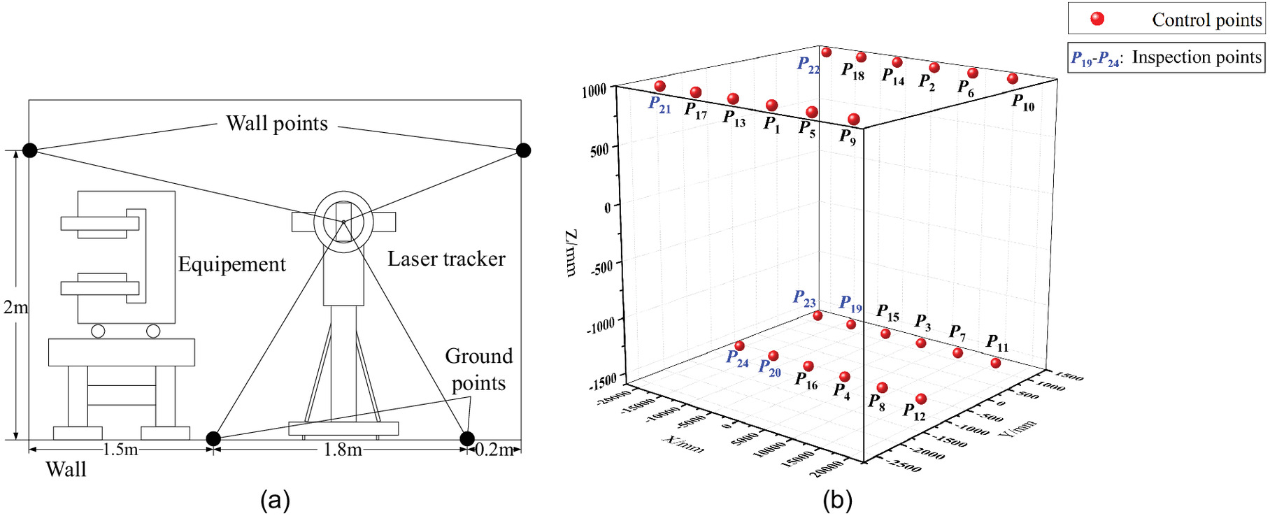
Fig. 1 shows the spatial layout of a single group of control points in the tunnel and the distribution of six groups of control points in the coordinate system of the tracker station. To guarantee the precision of the instrument, the distance between the two adjacent groups of points was 7 m, and the longest side did not exceed 18 m. The scale between the two periods of data was the same, the translation was (5.000, 8.000, and 0.300 m), the rotation vector was

\vec{g} = (\sqrt{3} / 3, \sqrt{3} / 3, \sqrt{3} / 3)

, and the rotation angle was 50°.

Taking the Leica laser tracker AT901-B as an example, the zenith angle measurement precision was

\pm {1.5}^{″}

, and the absolute ranging precision was

\pm 10 μ m

. The vertical coordinate precision was approximately

\pm 0.103 mm

within a range of 20 m, and the zenith distance was 45°, which is generally lower than the horizontal angle. The expectation of unequal precision error was set to 0. The standard deviations were randomly generated between 0 and 0.050 mm, 0 and 0.050 mm, and 0 and 0.100 mm, respectively, and were added to the

X

,

Y

, and

Z

coordinate components of the original observation values of points

P_{1} - P_{18}

in the second phase of data. This was performed to simulate the inconsistency of the precision of the coordinate components. The remaining points were not mixed with errors and were regarded as inspection points to check the precision of the coordinate transformation.

The following seven schemes were used to process the data. The number of simulations in each experiment was 500.

Scheme 1 shows the LS estimation. Scheme 2 and Scheme 3 chose the IGG3 weight function as the equivalent weight function. Scheme 4 and Scheme 5 take the Stuttgart weight function as the equivalent weight function. Scheme 6 and Scheme 7 adopt the Tukey weight function as the equivalent weight function. Scheme 2, Scheme 4, and Scheme 6 use the uniform scale factor to determine the threshold of the weight function. For Scheme 3, Scheme 5, and Scheme 7, we employed the coordinate component weighting method to estimate the scale factor of the coordinate components and determine the threshold of its weight function. The scale factor was estimated by the median function for Scheme 2 to Scheme 7. Stuttgart (Li and Yuan 2002) and Tukey function (Zhou et al. 1997) were expressed as follows:

Stuttgart : {\bar{p}}_{i} = \frac{p_{i}}{1 + {(\frac{| v_{i} |}{1.4 \cdot {\hat{σ}}_{v_{i}}})}^{d}} Tukey : {\bar{p}}_{i} = {\begin{cases} p_{i} {[1 - {(\frac{v_{i}}{e})}^{2}]}^{2} & | v_{i} | \leq e \\ 0 & | v_{i} | > e \end{cases}

(14)

where

p_{i}

= prior weight;

{\hat{σ}}_{v_{i}}

= standard deviation of residuals;

d = 3.5 + 82 / (81 + {(σ_{0} / σ_{pri or})}^{4})

;

σ_{pri or}

= prior standard deviation;

e = 4.685 σ_{0}

; and

σ_{0}

can be required by Eq. (10).

Table 2 lists the root mean square error (RMSE) of the parameters obtained by the seven schemes when the gross error was not mixed. Taking

λ

for example, the RMSE of

λ

can be calculated by

λ = \sqrt{(\sum_{i = 1}^{k} {(λ_{i} - λ_{t r u e})}^{2}) / k}

(15)

where

k

= number of experiments;

λ_{i}

and

λ_{tru e}

= calculated value for the

i

th experiment and true value, respectively.

Table 2. RMSE of estimated parameters for different schemes with zero outliers

Scheme	$λ / 10^{- 6}$	$Δ x / mm$	$Δ y / mm$	$Δ z / mm$	$a / 10^{- 6}$	$b / 10^{- 6}$	$c / 10^{- 6}$	$θ / (^{''})$
1	0.9	0.012	0.014	0.045	4.2	1.5	3.7	0.7
2	0.9	0.013	0.015	0.054	5.0	1.8	4.4	0.9
3	1.0	0.014	0.016	0.051	4.7	1.8	4.2	0.8
4	1.0	0.014	0.017	0.070	6.3	2.0	5.6	1.1
5	1.1	0.015	0.017	0.066	6.2	2.1	5.4	1.1
6	0.9	0.012	0.014	0.050	4.5	1.6	4.0	0.8
7	0.9	0.013	0.014	0.053	4.9	1.6	4.2	0.8

Table 2 shows that the LS estimation result was the best, and its parameters were the closest to the true value without abnormal data. After analysis, the LS method regards all observations as equal-weight observations and makes full use of all observation data in the process of solving parameters. This is an optimal parameter estimation method under the condition of only random errors. Schemes 2 to 7 led to the weight reduction of some observation data owing to their robustness. This reduced the efficiency of data utilization compared with LS, so the parameter results were slightly worse than LS, especially for Scheme 4 and Scheme 5. However, the difference was very small. From the result of the translation parameters, the RMSE of the

Z

direction was the largest among the seven schemes. This indicates that the precision of this direction was low and consistent with the actual situation.

To verify the robustness of different schemes, one, three, and five gross errors were added to the coordinate components of the second-phase data. The size was 0.500 mm, the positions were randomly generated, and the number of simulations was 500. The standard deviations of the unit weights of the robust schemes in the case of mixing gross errors are listed in Table 3.

Table 3. Comparison of

{\hat{σ}}_{0}

for robust schemes

Scheme	No gross error	One gross error	Three gross errors	Five gross errors
2	0.037	0.040	0.048	0.088
3	0.037	0.038	0.039	0.054
4	0.027	0.031	0.039	0.057
5	0.027	0.028	0.030	0.034
6	0.037	0.039	0.058	0.100
7	0.036	0.039	0.047	0.075

The

{\hat{σ}}_{0}

of Scheme 1 reached 0.040 mm when there was no outlier, which can be used as a reference to other schemes. It can be found intuitively that the results of Scheme 4 and Scheme 5 were the smallest, however, which was inconsistent with reality, and the accuracy was overestimated. When there were one and three gross errors in the data, only the results of Scheme 3 were basically consistent. This was equivalent to the results without gross errors, indicating that the method used in this study (Scheme 3) had better resistance to errors than the other schemes. Scheme 6 and Scheme 7 can keep robustness when one gross error is mixed. When the number of gross errors reached three or five, the robustnesses of Scheme 6 and Scheme 7 were weaker than Scheme 2 and Scheme 3. Compared with the other robust schemes, Scheme 6 has the lowest accuracy and weakest robustness. Furthermore, the results preliminarily show that the method based on coordinate component weighting has a higher tolerance than the traditional method when dealing with gross errors.

The method for selecting weight iterations achieves the purpose of robustness by reducing the weight of polluted observations. However, it has certain limitations. The robust estimation based on the LS principle allocates gross errors during the adjustment process, resulting in inaccurate residual results. Therefore, some weights of good observations are inevitably lowered, and

{\hat{σ}}_{0}

cannot fully demonstrate the effectiveness of the method. For example, when the data does not contain gross errors, although the

{\hat{σ}}_{0}

of the LS method is the largest, its results are optimal, and the parameters are the most accurate. Therefore, the advantages and disadvantages of this method need to be judged in combination with other indicators.

The RMSE of the parameters obtained by the six schemes after mixing with different numbers of gross errors are listed in Tables 4–6.

Table 4. RMSE of estimated parameters for different schemes with one outlier

Scheme	$λ / 10^{- 6}$	$Δ x / mm$	$Δ y / mm$	$Δ z / mm$	$a / 10^{- 6}$	$b / 10^{- 6}$	$c / 10^{- 6}$	$θ / (^{''})$
2	0.9	0.012	0.015	0.053	4.8	1.7	4.2	0.8
3	1.0	0.013	0.016	0.054	4.8	1.8	4.3	0.8
4	1.0	0.014	0.016	0.062	5.6	2.0	4.9	1.0
5	1.1	0.016	0.017	0.062	5.7	2.1	5.0	1.0
6	0.9	0.013	0.016	0.052	4.8	1.7	4.2	0.8
7	0.9	0.014	0.015	0.052	4.7	1.7	4.1	0.8

Table 5. RMSE of estimated parameters for different schemes with three outliers

Scheme	$λ / 10^{- 6}$	$Δ x / mm$	$Δ y / mm$	$Δ z / mm$	$a / 10^{- 6}$	$b / 10^{- 6}$	$c / 10^{- 6}$	$θ / (^{''})$
2	1.3	0.017	0.021	0.065	6.0	1.9	5.3	1.0
3	0.9	0.014	0.016	0.056	5.1	1.7	4.4	0.9
4	1.0	0.015	0.017	0.060	5.5	1.9	4.8	1.0
5	1.2	0.016	0.019	0.066	6.1	2.1	5.4	1.0
6	1.5	0.020	0.020	0.064	5.9	2.0	5.2	1.0
7	1.1	0.016	0.019	0.066	6.0	2.1	5.2	1.0

Table 6. RMSE of estimated parameters for different schemes with five outliers

Scheme	$λ / 10^{- 6}$	$Δ x / mm$	$Δ y / mm$	$Δ z / mm$	$a / 10^{- 6}$	$b / 10^{- 6}$	$c / 10^{- 6}$	$θ / (^{''})$
2	3.7	0.046	0.044	0.103	9.6	2.8	8.2	1.7
3	2.2	0.029	0.030	0.086	6.2	2.0	5.4	1.0
4	1.5	0.020	0.022	0.080	7.2	2.2	6.3	1.3
5	1.4	0.019	0.021	0.074	6.8	2.3	6.0	1.2
6	3.0	0.041	0.036	0.116	10.9	3.3	9.7	1.9
7	2.1	0.032	0.031	0.104	9.8	3.1	8.4	1.7

Tables 4–6 show the RMSE of the parameter estimation obtained by mixing different numbers of gross errors of the six schemes. Through observation, it can be determined that with an increase in the number of gross errors, the RMSE of the parameters of the six schemes gradually increased, and the results of the translation parameters in the

Z

direction were bigger than those in the

X

and

Y

directions. When there was one gross error, the results of the six schemes were very close to those without gross error, and all of them could maintain strong robustness. When the number of gross errors increased from one to five, the RMSE of the parameters from Scheme 2 to Scheme 7 started to increase by different degrees. The increased range of Scheme 4 and Scheme 5 was minimum, and that of Scheme 6 and Scheme 7 was the maximum. In addition, the results of Scheme 4 and Scheme 5 were basically consistent, indicating that the coordinate component weighting method has little effect on the Stuttgart function. When three and five outliers were mixed in the data, the results of Scheme 3 and Scheme 7 had better performance than Scheme 2 and Scheme 6, respectively, illustrating that the coordinate component weighting method can improve the robustness of the method by combining with IGG3 and Tukey weight functions, especially for Scheme 3. The RMSE of Scheme 3 increased relatively slowly with the increasing number of gross errors, the precision of the rotation angle reached

\pm 1^{″}

, and the translation parameter precision was within

\pm 0.100 mm

. This indicates that the weighting method used in this study is more robust than the traditional method.

To test the precision of the external coincidence of coordinate transformation of different schemes under the conditions of different gross errors, the coordinate transformation was conducted for six inspection points from

P_{19}

to

P_{24}

. The difference was compared to the true value of coordinates in the corresponding target coordinate system. To further verify the effectiveness of the coordinate component weighting method, Scheme 2 and Scheme 3 were adopted to perform the following tests. The results of the RMSE of the coordinate components of the inspection points are listed in Tables 7–9.

Table 7. RMSE of checkpoint coordinate components for different schemes with one outlier (mm)

Coordinate components	Scheme	$P_{19}$	$P_{20}$	$P_{21}$	$P_{22}$	$P_{23}$	$P_{24}$	RMS
$X$	2	0.017	0.017	0.023	0.025	0.023	0.023	0.022
$X$	3	0.019	0.019	0.026	0.028	0.026	0.025	0.024
$Y$	2	0.024	0.025	0.030	0.029	0.031	0.032	0.029
$Y$	3	0.025	0.026	0.032	0.031	0.033	0.033	0.030
$Z$	2	0.030	0.029	0.040	0.038	0.039	0.039	0.036
$Z$	3	0.030	0.030	0.041	0.039	0.040	0.039	0.037

Table 8. RMSE of checkpoint coordinate components for different schemes with three outliers (mm)

Coordinate components	Scheme	$P_{19}$	$P_{20}$	$P_{21}$	$P_{22}$	$P_{23}$	$P_{24}$	RMS
$X$	2	0.025	0.024	0.032	0.033	0.032	0.032	0.030
$X$	3	0.017	0.016	0.022	0.023	0.022	0.022	0.021
$Y$	2	0.032	0.032	0.036	0.035	0.040	0.040	0.036
$Y$	3	0.027	0.027	0.030	0.029	0.034	0.034	0.030
$Z$	2	0.036	0.034	0.045	0.045	0.045	0.043	0.042
$Z$	3	0.030	0.028	0.038	0.037	0.038	0.036	0.035

Table 9. RMSE of checkpoint coordinate components for different schemes with five outliers (mm)

Coordinate components	Scheme	$P_{19}$	$P_{20}$	$P_{21}$	$P_{22}$	$P_{23}$	$P_{24}$	RMS
$X$	2	0.076	0.075	0.098	0.099	0.098	0.097	0.091
$X$	3	0.047	0.046	0.058	0.059	0.060	0.060	0.055
$Y$	2	0.061	0.062	0.074	0.073	0.079	0.079	0.072
$Y$	3	0.041	0.041	0.053	0.051	0.052	0.053	0.049
$Z$	2	0.064	0.061	0.082	0.082	0.083	0.081	0.076
$Z$	3	0.043	0.040	0.054	0.057	0.055	0.052	0.051

Tables 7–9 show that the deviation of inspection points increased continuously with an increase in the number of gross errors. However, the RMSE of the coordinate components were all within 0.100 mm and larger for the

Z

direction than for the

X

and

Y

directions. When mixed in with one gross error, the RMSE of Scheme 2 was equivalent to that of Scheme 3, which is consistent with the parameter estimation results. When three and five gross errors were mixed in, the RMSE of the test points obtained by Scheme 3 was smaller than that of Scheme 2. Its advantages are more obvious with an increase in the number of gross errors. Fig. 1(b) shows that the distances from the test points to the conversion points vary. In contrast, the two inspection points

P_{19}

and

P_{20}

were closer to the conversion points, and their coordinate conversion errors were small. Inspection points

P_{21} - P_{24}

were farther away, and the conversion error was larger. This demonstrates that the farther the inspection point is from the conversion point, the larger the conversion error. Finally, the result of the outer coincidence precision of coordinate transformation shown in Tables 7–9 is consistent with the results of parameter estimation. This shows that the method used in this study has more advantages in dealing with gross errors and is more robust than the other methods examined.

In addition, the location of the blunders is also an important factor in robust estimation. To research the influence of blunders position on robust estimation, we designed experiments according to the random distribution (Situation a) and centralized distribution (Situation b) of gross errors, and Scheme 3 was used to deal with the above situations. The number of simulations was 500, and the RMSE of the parameters obtained by the two situations after mixing with four outliers are listed in Table 10.

Table 10. RMSE of estimated parameters for different situations with four outliers

Situation	$λ / 10^{- 6}$	$Δ x / mm$	$Δ y / mm$	$Δ z / mm$	$a / 10^{- 6}$	$b / 10^{- 6}$	$c / 10^{- 6}$	$θ / (^{''})$
a	1.1	0.016	0.017	0.058	5.0	1.9	4.6	0.9
b	1.0	0.018	0.021	0.120	10.6	1.9	9.7	1.9

Table 10 shows that the results of Situation a are better. The RMSE of the scale parameter in both situations was basically the same. For the translation parameters, the results of Situation a were smaller than that of Situation b, especially in the Z direction, the result of Situation a was only 0.058 mm, while the result of Situation b was 0.120 mm. This is still the case for rotation parameters, and the results of Situation b were about twice as large as the results of Situation a. The standard deviations of the unit weight of Situation a and Situation b were 0.041 mm and 0.048 mm, respectively, demonstrating that the precision of Situation a is higher than Situation b. The presented results show that it is more difficult to suppress the gross error of centralized distribution than that of random distribution.

Case Analysis

The measured data from two stations in the tunnel control network of the accelerator project, including 20 common points, and the distribution of control points is shown in Fig. 2.

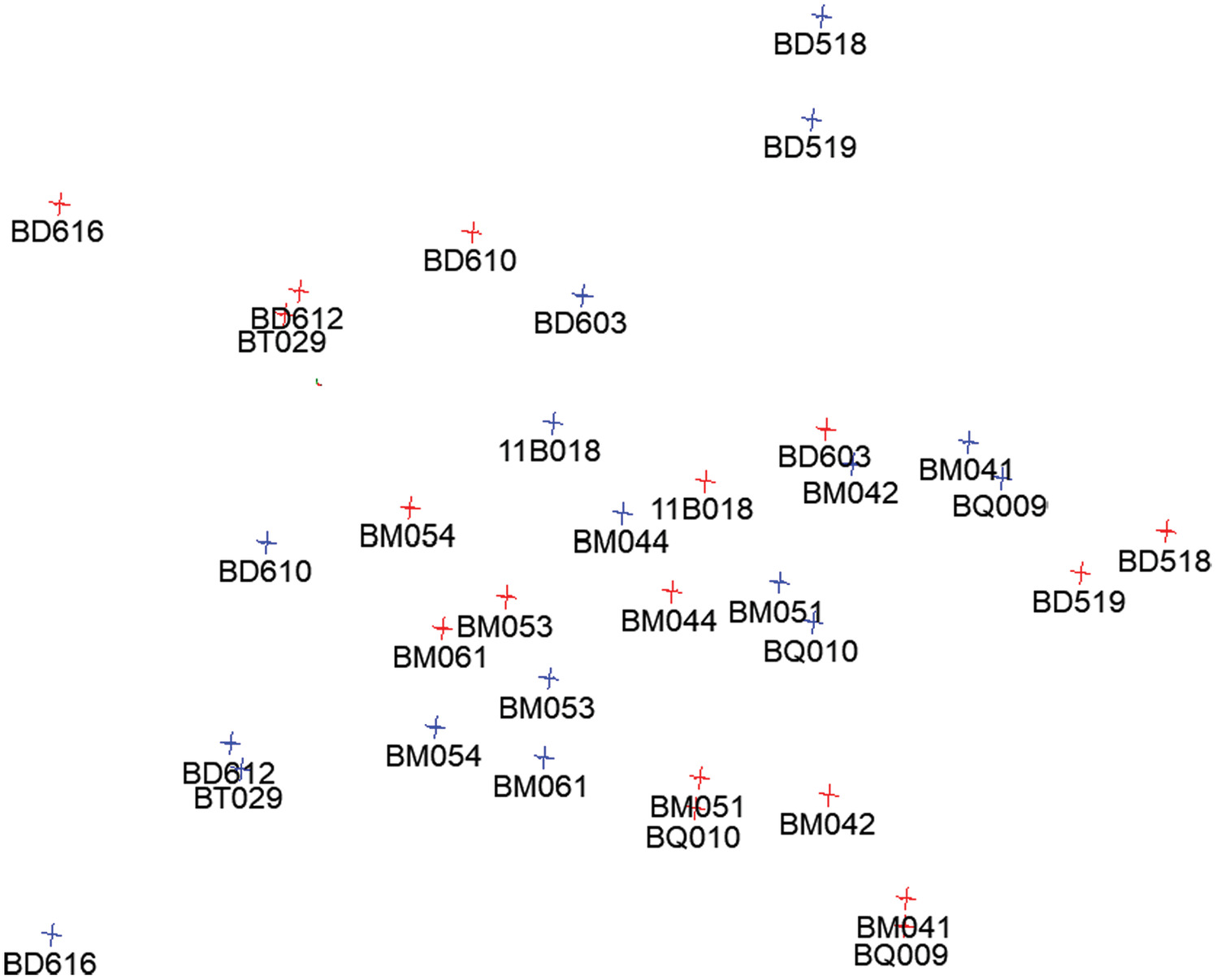
Fig. 2. Distribution of control point locations.

The data were processed using Schemes 1–3 and the method of Guo et al. (2020). The residuals of the common point coordinate components are shown in Fig. 3.

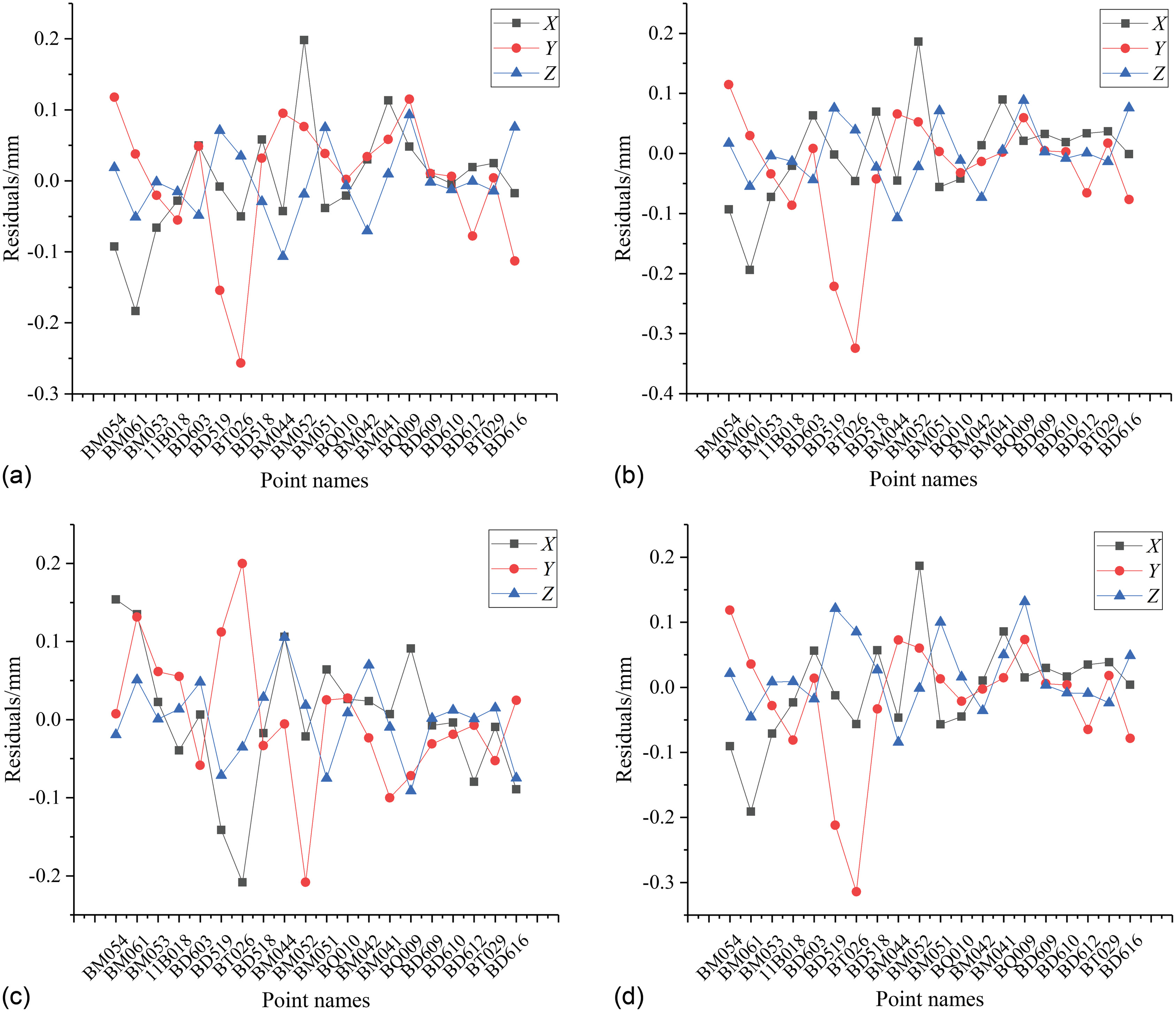
Fig. 3. Coordinate component residuals of (a) Scheme 1; (b) Scheme 2; (c) Guo et al. (2020); and (d) Scheme 3.

Fig. 3 shows the coordinate component residual results of the four methods. The figure shows that the errors were mainly distributed on points BM054, BM061, BD519, BT026, and BM044. Among these points, the residual results of Schemes 1–3 have good consistency. This is particularly true for Schemes 2 and 3 where the residual results were approximately equal. The residuals of most points were maintained at approximately

\pm 0.100 mm

, indicating that the robust estimation method is well resistant to error effects. Although the residual results of Guo et al. (2020) are different from those of other methods, the position of the main distribution of larger errors is the same as those of the other methods.

Robust estimation eliminates gross errors by reducing their weights to a small value or even to zero. To verify the rationality of the coordinate component weighting method, the gross errors eliminated in Scheme 2 and Scheme 3 and the corresponding residuals and weight results are shown in Table 11.

Table 11. Gross errors and their residuals and weights

Coordinate components	Scheme	Residuals (mm)				Weights
Coordinate components	Scheme	BM061	BD519	BT026	BM052	BM061	BD519	BT026	BM052
$X$	2	$- 0.194$	$- 0.002$	$- 0.046$	0.186	1.000	1.000	1.000	1.000
$X$	3	$- 0.194$	$- 0.001$	$- 0.046$	0.186	0.000	1.000	1.000	0.011
$Y$	2	0.029	$- 0.221$	$- 0.324$	0.052	1.000	0.000	0.000	1.000
$Y$	3	0.028	$- 0.220$	$- 0.323$	0.051	1.000	0.000	0.000	1.000
$Z$	2	$- 0.055$	0.076	0.039	$- 0.022$	0.000	1.000	1.000	0.000
$Z$	3	$- 0.047$	0.076	0.041	$- 0.012$	1.000	1.000	1.000	1.000

Table 11 shows that the points with gross errors in the two schemes include BM061, BD519, BT026, and BM052. In terms of residuals, the coordinate components of these four points in

X

,

Y

,

Y

, and

X

directions were the largest (

\min = 0.186

and

\max = 0.324

), which should be judged as gross errors. However, the weight results of Scheme 2 show that the weights in the

X

direction of points BM061 and BM052 were not equal to 0, and the gross error position identified by them was in the

Z

direction with small residuals, so the position of gross errors was judged incorrectly. The weight of Scheme 3 in the direction with the largest residual of four points was 0, indicating that the weight results were reasonable and reliable.

To further verify the advantages and disadvantages of the results of the different methods, the LS method was used to process the data. After obtaining the residuals, the points with the largest coordinate component residuals were successively removed until the maximum absolute value of the coordinate component residuals of all points was within 0.100 mm. After removing points BM054, BM061, BD519, BT026, BM044, and BM052, the remaining 14 points were handled by LS. Their parameter estimations were regarded as theoretical values and compared with the other methods. The results of the translation parameters are presented in Table 12.

Table 12. Difference between the calculated value and the theoretical value and

{\hat{σ}}_{0}

(mm)

Scheme	$d Δ x$	$d Δ y$	$d Δ z$	$S$	${\hat{σ}}_{0}$
1	$- 0.019$	0.001	$- 0.034$	0.039	0.079
2	0.008	$- 0.016$	$- 0.027$	0.033	0.054
3	0.004	$- 0.015$	$- 0.019$	0.025	0.046
Guo et al. (2020)	$- 0.002$	$- 0.009$	$- 0.032$	0.033	0.074

Note: $S$ is the RMS of the difference between the translation parameter estimation and the theoretical parameter value.

Table 12 shows that after removing the larger error points,

{\hat{σ}}_{0}

reached 0.045 mm (theoretical value). A better parameter estimation result was acquired when the LS estimation was performed on the remaining points. However, the other four schemes produced results in which all the error points were not removed. Consequently, the

{\hat{σ}}_{0}

results were larger owing to the interference of the error points. LS estimation is not robust, so the parameter estimation result of Scheme 1 was the least accurate of the examined methods, having the largest S (0.039 mm). Scheme 2 produced the same

S

as in the Guo et al. (2020) method, but the

{\hat{σ}}_{0}

of Guo et al. (2020) was larger. After analysis, because of the randomness of the method used by Guo et al. (2020), the parameter estimation may fall into a local optimum when the number of error points is larger. By comparison, the parameter results obtained by the method in this study (Scheme 3) were the closest to the theoretical results, and the

{\hat{σ}}_{0}

was the smallest. This demonstrates strong robustness, proving the effectiveness of the method.

Conclusion

Based on Rodrigues’ formula, a linearization model of the coordinate transformation was derived. The proposed method is not limited by the rotation angle, the model is simple and efficient, the weight determination method is simple, and it is not affected by empirical parameters. Considering the difference in the precision of each coordinate component of common points, the idea of coordinate component weighting was proposed. The median function was utilized to obtain the scale factor of the coordinates in different directions to determine the threshold of the weight function. Taking the tunnel control network of particle accelerator engineering as an example, a simulation experiment and case analysis were conducted, and comparisons with the existing methods were performed. The results show that the method proposed in this study is more robust than the traditional methods and has higher coordinate transformation precision. In addition, it is more difficult to suppress the gross error of centralized distribution than that of random distribution.

Data Availability Statement

All data, models, and code that support the findings of this study are available from the corresponding author upon reasonable request.

Acknowledgments

The writers thank the anonymous reviewers and the editor for their valuable comments on the manuscript. The work described in this paper was substantially supported by the National Natural Science Foundation of China (Project No. 41974216). The authors are grateful to engineer Zhao Wenbin for providing the data required for the research.

References

Chen, Y., Y. Shen, and D. Liu. 2004. “A simplified model of three dimensional-datum transformation adapted to big rotation angle.” Geomatics Inf. Sci. Wuhan Univ. 29 (12): 1101–1105.

Google Scholar

Eshagh, M., L. Sjöberg, and R. Kiamehr. 2007. “Evaluation of robust techniques in suppressing the impact of outliers in a deformation monitoring network—A case study on the Tehran Milad tower network.” Acta Geod. Geophys. Hung. 42 (4): 449–463. https://doi.org/10.1556/AGeod.42.2007.4.6.

Google Scholar

Fang, X., L. Huang, and W. Zeng. 2018. “On an improved iterative reweighted least squares algorithm in robust estimation.” Acta Geod. Cartographica Sin. 47 (10): 1301–1306. https://doi.org/10.11947/j.AGCS.2018.20170576.

Google Scholar

Felus, F., and R. Burtch. 2009. “On symmetrical three-dimensional datum conversion.” GPS Solut. 13 (1): 65–74. https://doi.org/10.1007/s10291-008-0100-5.

Google Scholar

Grafarend, E. W., and J. Awange. 2003. “Nonlinear analysis of the three-dimensional datum transformation.” J. Geod. 77 (1–2): 66–76. https://doi.org/10.1007/s00190-002-0299-9.

Google Scholar

Greenfeld, S. 1997. “Least squares weighted coordinate transformation formulas and their applications.” J. Surv. Eng. 123 (4): 147–161. https://doi.org/10.1061/(ASCE)0733-9453(1997)123:4(147).

Google Scholar

Guo, Y., Z. Li, and H. He. 2020. “A simplex search algorithm for the optimal weight of common point of 3d coordinate transformation.” Acta Geod. Cartographica Sin. 49 (8): 1004–1013. https://doi.org/10.11947/j.AGCS.2020.20190409.

Google Scholar

Jazar, R. N. 2007. Theory of applied robotics: Kinematics, dynamics, and control. New York: Springer.

Crossref

Google Scholar

Li, D., and X. Yuan. 2002. Error processing and reliability theory. Wuhan: Wuhan University Press.

Google Scholar

Liu, C., B. Wang, and X. Zhao. 2018. “Three-dimensional coordinate transformation model and its robust estimation method under Gauss-Helmert model.” Geomatics Inf. Sci. Wuhan Univ. 43 (9): 1320–1327. https://doi.org/10.13203/j.whugis20160348.

Google Scholar

Lu, J., Y. Chen, B. Li, and X. Fang. 2014. “Robust total least squares with reweighting iteration for three-dimensional similarity transformation.” Surv. Rev. 46 (334): 28–36. https://doi.org/10.1179/1752270613Y.0000000050.

Google Scholar

Lv, Z., J. Wu, and Y. Gong. 2016. “Improvement of a three-dimensional coordinate transformation model adapted to big rotation angle based on quaternion.” Geomatics Inf. Sci. Wuhan Univ. 41 (4): 547–553. https://doi.org/10.13203/j.whugis20140171.

Google Scholar

Tao, Y., J. Gao, and Y. Yao. 2016. “Solution for robust total least squares estimation based on median method.” Acta Geod. Cartographica Sin. 45 (3): 297–301. https://doi.org/10.11947/j.AGCS.2016.20150234.

Google Scholar

Uygur, S. O., O. Akyilmaz, and C. Aydin. 2021. “Solution of nine-parameter affine transformation based on quaternions.” J. Surv. Eng. 147 (3): 04021011. https://doi.org/10.1061/(ASCE)SU.1943-5428.0000364.

Google Scholar

Wu, Z., W. Luo, and J. Li. 2014. “On position of gross errors of common points in coordinate transformation and reducing influence of gross errors.” J. Geod. Geodyn. 34 (1): 118–122. https://doi.org/10.14075/j.jgg.2014.01.011.

Google Scholar

Xu, B., J. Gao, and Z. Li. 2015. “The application of the total least squares algorithm based on reweighting iteration to the three-dimensional coordinates.” J. Geod. Geodyn. 35 (4): 693–696. https://doi.org/10.14075/j.jgg.2015.04.033.

Google Scholar

Yang, L., and Y. Shen. 2020. “Robust M estimation for 3D correlated vector observations based on modified bifactor weight reduction model.” J. Geod. 94 (3): 1–17. https://doi.org/10.1007/s00190-020-01351-1.

Google Scholar

Yang, Y. 1994. “Robust estimation for dependent observations.” Manuscr Geod. 19 (1): 10–17.

Google Scholar

Yao, J., B. Han, and Y. Yang. 2006. “Applications of lodrigues matrix in 3d coordinate transformation.” Geomatics Inf. Sci. Wuhan Univ. 31 (12): 1094–1096.

Google Scholar

Yu, G., G. Feng, and J. Zhang. 2018. “Discussion on plane coordinate transformation based on barycentre datum.” GNSS World China 43 (1): 15–18. https://doi.org/10.13442/j.gnss.1008-9268.2018.01.003.

Google Scholar

Zeng, W., and B. Tao. 2003. “Non-linear adjustment model of three-dimensional coordinate transformation.” Geomatics Inf. Sci. Wuhan Univ. 28 (5): 566–568.

Google Scholar

Zhou, J., Y. Huang, and Y. Yang. 1997. Robust least squares. Wuhan: Huazhong University of Science and Technology Press.

Google Scholar

Information & Authors

Information

Published In

Journal of Surveying Engineering

Volume 149 • Issue 3 • August 2023

Copyright

This work is made available under the terms of the Creative Commons Attribution 4.0 International license, https://creativecommons.org/licenses/by/4.0/.

History

Received: Aug 24, 2022

Accepted: Feb 7, 2023

Published online: Apr 10, 2023

Published in print: Aug 1, 2023

Discussion open until: Sep 10, 2023

Authors

Affiliations

Zhonghe Liu https://orcid.org/0000-0001-7190-9244 [email protected]

Ph.D. Student, School of Geospatial Information, Information Engineering Univ., Zhengzhou 450001, China. ORCID: https://orcid.org/0000-0001-7190-9244. Email: [email protected]

View all articles by this author

Zongchun Li [email protected]

Professor, School of Geospatial Information, Information Engineering Univ., Zhengzhou 450001, China (corresponding author). Email: [email protected]

View all articles by this author

Jiahuan Ran

Master’s Student, School of Geospatial Information, Information Engineering Univ., Zhengzhou 450001, China.

View all articles by this author

Metrics & Citations

Metrics

Citations

Download citation

If you have the appropriate software installed, you can download article citation data to the citation manager of your choice. Simply select your manager software from the list below and click Download.

Robust Solution for Coordinate Transformation Based on Coordinate Component Weighting

Abstract

Introduction

Algorithm Principle

Coordinate Transformation Model

Initial Value Calculation of Parameters

Coordinate Component Weighting

Calculation Procedure

Simulation Test and Case Analysis

Simulation Test

Case Analysis

Conclusion

Data Availability Statement

Acknowledgments

References

Information & Authors

Information

Published In

Copyright

History

Authors

Affiliations

Metrics & Citations

Metrics

Citations

Download citation

View Options

Media

Figures

Other

Tables

PREVIOUS ARTICLE

NEXT ARTICLE

Verify Phone

Congrats!

Abstract

Introduction

Algorithm Principle

Coordinate Transformation Model

Initial Value Calculation of Parameters

Coordinate Component Weighting

Calculation Procedure

Simulation Test and Case Analysis

Simulation Test

Case Analysis

Conclusion

Data Availability Statement

Acknowledgments

References

Information

Published In

Copyright

History

Authors

Affiliations

Metrics

Citations

Download citation

Figures

Other

Share

Copy the content Link

Share with email

Share

Request Username

Create a new account

Change Password

Password Changed Successfully

Verify Phone

Congrats!