An Investigation of Climate Change Effects on Design Wind Speeds along the US East and Gulf Coasts

Tropical cyclones (TCs) are a significant hazard to infrastructure in the United States, and TC winds govern design wind speeds for much of the US Gulf and Atlantic coasts. It is now widely accepted that TC intensity will increase with climate change (Committee on Adaption to a Changing Climate 2018; Emanuel 2021; Knutson et al. 2020; Task Committee on Future Weather and Climate Extremes 2021; Walsh et al. 2019). This increase will likely lead to increased wind speeds along the Gulf and Atlantic coasts of the United States (Esmaeili and Barbato 2021), but the current ASCE 7 design wind speed maps do not account for climate change effects ([ASCE 7-22 (ASCE 2021)]. As a result, numerous structures are potentially being designed with greater levels of risk than ASCE 7-22 originally intended. The primary objectives of this study were to investigate (1) the expected increase in design wind speeds from increased TC activity due to climate change; and (2) the resulting levels of risk if this effect of climate change is not accounted for. This study uses state-of-the-art synthetic TC data generated from the Coupled Model Intercomparison Project Phase 6 (CMIP6) under the shared socioeconomic pathway (SSP) 5–8.5 to implement nonstationary design wind speed calculations. The design wind speeds in ASCE 7-22 are specified based on mean return intervals (MRIs), under the stationary assumption. This paper focuses on design wind speeds based on lifetime exceedance probability (LEP) for the nonstationary condition. An MRI is the average time between hazard events of a given intensity level, while the LEP is the probability that a given intensity level will be exceeded over the design lifetime of a structure.

In the introduction of this paper, we describe the nonstationary statistical methods and the synthetic TC data used here, contrasting them with those of previous studies. In the next section, we describe the methodology used to generate the wind speed data and to statistically analyze it. In the following section, the model is evaluated against both historical data and the ASCE 7-22 design wind speeds. In our results and discussion section, we discuss, the increase in design wind speeds with climate change, the resulting LEPs if no action is taken, and the effective risk categories associated with the resulting LEPs. The next section shows the increases in design wind speeds using an MRI-based rather than the LEP-approach and features a comparison between those two approaches, as well as to other studies that have attempted to predict increases in the MRI-based design wind speed due to climate change. Finally, we highlight areas of future research and potential challenges to changing the design code before delivering our conclusions.

The ASCE 7-22 design wind speed maps give wind speeds to be used for structural design purposes. There are four maps for the contiguous US, one for each of Risk Categories I, II, III, and IV, with higher risk categories corresponding to lower permitted levels of risk. The four maps show contours of the 3-s gust wind speed for the open terrain at a height of 10 m for MRIs of 300, 700, 1,700, and 3,000 years, respectively, representing ultimate loading conditions rather than service-level conditions. Designing for an MRI of 1,700 years, for example, means that the probability of experiencing wind speeds greater than the design level in a given year is $1/\mathrm{1,700}$. Even though the probability of occurrence for any given year is low, the cumulative probability of occurrence grows as a function of time. As a result, the probabilities that the specified design wind speeds will be exceeded within 50 years are 0.15, 0.07, 0.03, and 0.017 for Risk Categories I–IV, respectively (ASCE 7-22). If the time period considered is the design lifetime, this cumulative probability may be called the LEP (Xu et al. 2020).

The eastern United States is a mixed-wind environment, with TCs, thunderstorms, and large-scale weather systems contributing to extreme wind speeds. Twisdale and Vickery (1992) showed that failing to separate different wind sources in a mixed-wind environment leads to underestimates of extreme wind speeds. Thus, TC and non-TC winds were handled separately in ASCE 7-22. The non-TC wind speed data was sourced from weather station records while the TC wind speed data was generated using synthetic TCs, which are discussed in the “Synthetic Tropical Cyclone Modeling” section.

A stationary climate was assumed for the ASCE 7-22 design wind speed maps (ASCE 7-22); however, Cui and Caracoglia (2016) suggested climate nonstationarity be assumed under representative concentration pathway (RCP)4.5 and RCP8.5, the latter of which is consistent with the SSP5-8.5 scenario considered in this study. Because MRIs vary with time in a nonstationary climate, Xu et al. (2020) proposed specifying design wind speeds in terms of LEPs instead of MRIs. As MRIs and LEPs are equivalent descriptors of risk in a stationary climate, it is natural to apply LEPs in a nonstationary climate to ensure that a set risk is not exceeded over the lifetime of a structure (Rootzén and Katz 2013; Xu et al. 2020). Also, as discussed by Xu et al. (2020), LEP-based design is consistent with the traditional stationary design in conserving the risk of failure measured by various probabilistic metrics (Buchanan et al. 2016; Hunter 2012).

One challenge with LEP-based design is that targeting the cumulative exceedance probability (e.g., 0.03 for 50-year lifetime) corresponding to a stationary annual exceedance probability ($1/\mathrm{1,700}$) may lead to the annual exceedance probability being greater than the stationary annual exceedance probability ($1/\mathrm{1,700}$) in some years (e.g., toward the end of the lifetime if the climate change impact increases continuously over time). A more conservative approach would be to target the highest annual MRI over the design lifetime (e.g., at the end of the lifetime) so that the annual exceedance probabilities currently specified in ASCE 7-22 would not be exceeded. This paper primarily used the LEP-based approach, with a section dedicated to the MRI-based approach for comparison.

A large sample of TC wind speed data is required to obtain a reliable extreme value distribution of TC wind. Due to the lack of sufficient observational data, various models have been developed to simulate synthetic TC events. The synthetic method used in the development of the ASCE 7-22 design wind speed maps was first described in Vickery et al. (2000) and later updated in Vickery et al. (2009b; ASCE 7-22). To generate a synthetic TC using this approach (Vickery et al. 2000, 2009b), the initial location, date, time, bearing, translation speed, and central pressure deficit were sampled from the historical best track record. Then, the track and pressure deficit along the track were simulated based on statistical models and environmental variables such as sea surface temperature (SST). Using the simulated parameters, the radius of maximum winds and the Holland $B$ parameter were determined, allowing the calculation of surface wind speeds at any point and time along the track using a parametric model, such as the Holland (1980) model, of gradient winds. Because the tracks generated using the method from Vickery et al. (2009b) rely mainly on historical TC data, the method’s ability to account for potential effects of climate change on TC activity in the future is limited.

In this study, we employed synthetic TC data generated from the synthetic method developed by Emanuel et al. (2006, 2008), which can generate synthetic TCs driven by comprehensive climate conditions involving the environmental wind and humidity, thermodynamic state of the atmosphere, and thermal stratification of the ocean. In this approach (Emanuel et al. 2008), synthetic TCs are formed by uniformly generating weak storms or seeds over time and location except for within 2° latitude of the equator. Most of those storms quickly dissipate due to unfavorable conditions, but those that reach TC status then follow a track determined by large-scale wind patterns, generated from the statistics of the projected environmental winds. Storm intensity along those tracks is then calculated using a deterministic coupled ocean-atmosphere model (Emanuel et al. 2008). This synthetic TC model does not rely on the historical track database but rather generates synthetic storms that are in statistical agreement with observations (Emanuel et al. 2006; Hallegatte 2007). The TC wind (Yeo et al. 2014; Xu et al. 2020), surge (Marsooli et al. 2019), and joint (Gori et al. 2022) hazards generated using this model compare well with the historical observations and are compatible with geologic evidence (Lin et al. 2014). While the method in Vickery et al. (2009b) can account for the effect of climate change on storm intensity, this method accounts for also the influence of climate change on TC genesis (i.e., frequency) and track, making it a more robust methodology in the context of climate change. This synthetic TC model has been applied to assess TC wind hazard (Xu et al. 2020), storm surge hazard (Lin et al. 2019; Marsooli et al. 2019), rainfall hazard (Emanuel 2017), and joint hazard (Gori et al. 2022; Xi et al. 2023) under climate change.

The synthetic TC data used in this study was obtained from Gori et al. (2022) who used the method from Emanuel et al. (2008) to generate synthetic TC data for 1,500 years under the historical climate from 1984 to 2015 based on the National Centers for Environmental Prediction (NCEP). The simulated storm wind intensity compares well with the observation over the same period for various regions along the US Gulf and East coasts, although the model appears to underestimate the wind intensity for the Northeast coast, given the sampling limitation in both simulation and observation for this region. See Supplementary Materials Fig. S1. The same method was used to generate a set of bias-corrected synthetic TC data for 1,000 years of the future climate of 2070–2100 based on 24,000 years of simulations driven by eight CMIP6 models under the emission scenario SSP5-8.5. In the bias correction process, the outputs of each of the global climate models are scaled so that the intensity distribution and landfall frequency given by the model for the historical period are consistent with those given by the NCEP analysis. A single set of data ($\sim \mathrm{1,500}\mathrm{years}$) was then compiled from the eight models, weighted according to their accuracy in estimating the TC intensity return levels compared to the NCEP analysis. Further information about the TC modeling and bias correction process can be found in Gori et al. (2022). The model projects significant increases in landfall storm intensity and frequency, leading to significant increases in projected wind hazards. See Supplementary Materials Tables S1 and S2.

Previous studies have investigated the increase in wind speeds for the United States from increased TC winds. Mudd et al. (2014) studied the increase in design wind speeds for the Northeastern United States in year 2100 under RCP8.5. This study used the synthetic TC modeling approach from Vickery et al. (2009b) with SST being the only nonstationary parameter. Using a similar approach, Ellingwood and Lee (2016) estimated the increase in TC winds due to climate change over a 200-year service life for a building in Miami, and Cui and Caracoglia (2016) studied increases in TC winds and lifetime costs on tall buildings from increases in TC wind damage. Like Mudd et al. (2014), Snaiki and Wu (2020a) studied the increase in design wind speeds in the Northeastern United States, but that study used the synthetic TC model established in Snaiki and Wu (2020b), which accounts for the effects of changes in SST, wind shear, and convective instability. Finally, Esmaeili and Barbato (2021) explored the effects of climate change on design wind speeds for the Atlantic and Gulf coasts. Unlike the other studies reviewed in this section, Esmaeili and Barbato (2021) used a site-specific rather than a basin-wide approach to generate synthetic TC data, but that study made a similar assumption that every nonstationary variable was a function of SST. The design wind speeds were then calculated for the year 2060 according to the ASCE 7-22 MRIs.

Crucially, many of these studies are limited in their application for informing design wind speeds for the US East and Gulf coasts. Mudd et al. (2014) and Snaiki and Wu (2020a) studied only the effects on the Northeastern United States, and Snaiki and Wu (2020a) and Esmaeili and Barbato (2021) considered only coastal locations. Cui and Caracoglia (2016) considered only the effects of TCs, whereas the ASCE 7 design wind speeds include contributions from both TC and non-TC events. Additionally, none of these studies considered the LEP-based approach for calculating design wind speeds, nor did they attempt to calculate the levels of risk associated with failing to update the wind provisions in the code, as done in this study.

The synthetic TC data from Gori et al. (2022) was used to calculate the wind speeds at every US county that experienced more than 100 TCs passing within 200 km of it in both the past and future climate simulations (i.e., with TC rate greater than 0.1/year during the 1,000-year simulations). Each county was represented by a single internal point, which generally corresponded to its centroid (USCB 2021; USCB 2022). For each 2-h time step of each synthetic TC, the gradient wind speed at each county within 200 km of the TC center was calculated using the widely used Holland (1980) gradient wind model. The surface wind speeds were then determined parametrically. An empirically determined surface wind reduction factor of 0.85 was used (Batts et al. 1980). The inflow angle was calculated using the method from Bretschneider (1972). Finally, the background wind contribution used was 0.55 of the TC translation speed at 20° counterclockwise from its bearing (Lin and Chavas 2012). See Lin and Chavas (2012) for further discussion on hurricane parametric modeling and sensitivity analyses for the parameters aforementioned. This procedure gave the surface wind speeds over open water, which were converted to wind speeds over open terrain according to Simiu (2011), using roughness lengths of 0.0002 and 0.03 m for open water and open terrain, respectively (Davenport et al. 2000).

At each location, the maximum wind speeds from the synthetic TCs were fitted to a generalized Pareto distribution (GPD) using a peaks-over-threshold approach. The GPD (Coles 2001; Davison and Smith 1990) is widely used to model meteorological hazards, including extreme winds (e.g., Lombardo et al. 2009;Xu et al. 2020), heavy rainfall (Villarini et al. 2011), floods (Villarini and Smith 2010), and storm surges (e.g., Walton 2000; Lin et al. 2010). A GPD is defined by the threshold $u$, the scale parameter $\sigma$, and the shape parameter $\xi$, with the last variable particularly influencing the distribution’s behavior. If $\xi <0$, the tail of the distribution is bounded, whereas if $\xi =0$, the tail is unbounded and decays exponentially, and if $\xi >0$, the tail is also unbounded but decays polynomially. These cases are known as the Reverse Weibull, Gumbel, and Fréchet distributions, respectively. Eq. (1) shows the exceedance probability of a GPD, where $P(X>x)$ is the probability of exceeding $x$ and ${\zeta }_u$ is the probability of threshold exceedance as follows:

The threshold for each GPD was selected by minimizing the root mean square error (RMSE) of the fitted distribution over a range of potential thresholds. The minimum potential threshold was the 70th percentile of the data while the maximum potential threshold yielded no fewer than 20 exceedances of the threshold. $\xi$ was constrained to be less than or equal to 0 as the Fréchet distribution may overestimate wind speeds at long return periods (Yeo et al. 2014).

Because each location had extreme wind speed distributions only for the past (1984–2015) and future (2070–2100) climates, the three parameters of the GPD, $u$, $\sigma$, and $\xi$, were linearly interpolated each year, beginning with the past climate in 2000 and ending with the future climate in 2100. Cui and Caracoglia (2016) also linearly interpolated their GPD parameters to achieve nonstationarity over time, and Das et al. (2020) showed that this interpolation method is valid for the generalized extreme value distribution (GEV), a distribution related to the GPD. Assuming the future climate condition would occur at the end rather than the median year of the future climate simulation is not a conservative assumption; however, since the synthetic TC data are based upon the conservative SSP5-8.5 assumption, we chose to use this nonconservative assumption to be able to calculate design wind speeds for longer design lifetimes (See “Structure Lifespan” section).

Non-TC winds in the United States may increase with climate change, but further research is needed to more accurately determine the effects of climate change on extratropical cyclones (ETCs) (Colle et al. 2015; Lin et al. 2019) and thunderstorms (Seeley and Romps 2015; Trapp 2021). Due to that uncertainty and the fact that TC winds dominate the wind distribution for most of the study areas (see discussion in the “Non-TC Modeling” section), we assume a stationary distribution of non-TC winds. The non-TC wind speed data was sourced from Pintar et al. (2015) to reflect what is currently used in ASCE 7-22. That study provided an R package that calculates the MRIs for non-TC winds, and $\xi$ of the GPD wind speed distribution can be set to 0, $-0.05$, or $-0.10$ (Pintar et al. 2015). In this study, $\xi$ was set to 0 in accordance with the ASCE 7-22 methodology.

In a nonstationary climate, the design time horizon, or service lifespan of a structure, is crucial to determining the design wind speed. However, service life is often not considered in the United States, and most structures are assumed to function for 50–75 years (Ellingwood and Lee 2016), with 50 years being the default service life used in ASCE 7-22. We focus on four indicative scenarios that combine two possible lifespans and two possible build years, as summarized in Table 1. The year 2000 was chosen as the build year for structures that already exist while planned structures were assumed to be built in 2030. The average lifespan was chosen to be 50 years to match ASCE 7-22, and the longer lifespans of 70 years and 100 years were defined as ending in 2100, the last year with synthetic TC data. For each lifetime, a stationary design wind speed was also calculated for comparison.

The LEP-based approach was adopted from Xu et al. (2020). The MRIs given in the ASCE 7-22 design wind speed maps were converted to LEPs using Eq. (2), where $T$ is the specified MRI, $m$ is the design lifetime in years, and $p$ is the LEP as follows:

For each scenario, that LEP was used to calculate the design wind speed $x_d$ from Eq. (3), where $P(X^{NTC}\le x_d)$ is the annual nonexceedance probability from non-TC winds, and $P(X_n\le x_d)$ is the annual nonexceedance probability from TC winds in the $n$th year (Xu et al. 2020) as presented in the following expression:

To ensure that the model produced reasonable results, TC wind return level curves were generated for four coastal National Oceanographic and Atmospheric Agency (NOAA) weather stations and compared with the historical record. The stations studied were New Orleans Airport, Tampa International Airport, Miami International Airport, and John F. Kennedy (JFK) International Airport (NOAA 2022a, b, c, d). The coordinates of the actual stations were used rather than the county internal points to remove that discrepancy for this comparison. The historical record was compiled by extracting the maximum wind speed at each station for every TC that passed within 200 km of it from 1984 to 2015, per the NOAA Historical Hurricane Tracks website (NOAA n.d). Each station transitioned from recording peak gust wind speeds to recording peak 5-s gust wind speeds in either 1995 or 1996. We assumed that the earlier data consisted of 3-s gust wind speeds, and the later data was converted from 5-s gust wind speeds to 3-s gust wind speeds following Simiu (2011).

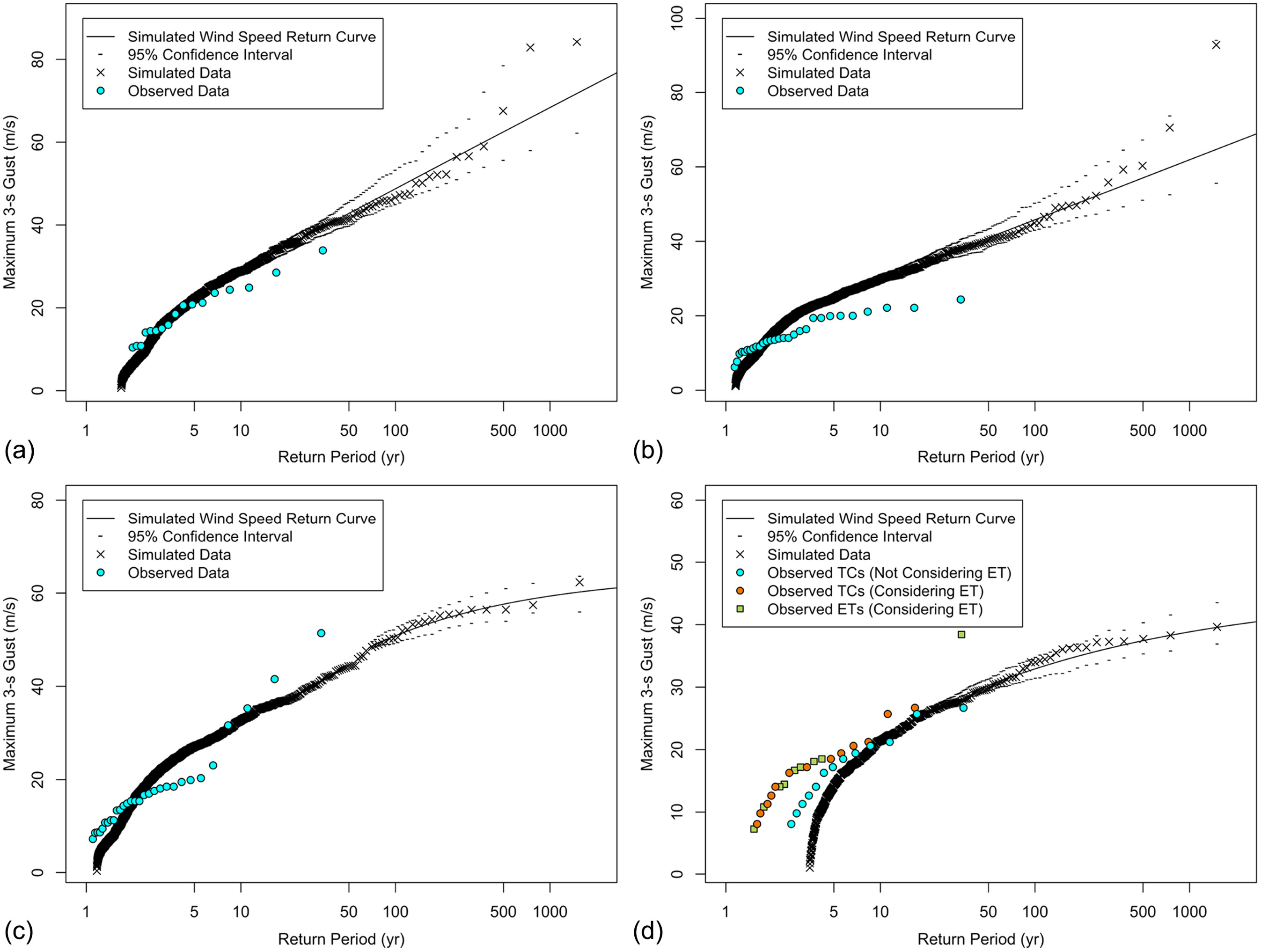
Fig. 1 shows the generated return level curves for the synthetic data in the control simulation compared with the historical observations (1984–2015) for the selected locations. The control return levels are generally consistent with the historical records, and the historical records are especially well-captured by the model for New Orleans. The model overestimates return levels for Tampa, while at Miami, it overestimates return levels for low return periods (10 years or lower) and underestimates return levels for longer return periods, although there are fewer observational data points to show that. The simulated TC winds at Miami and JFK follow the Reverse Weibull distribution, while those at New Orleans and Tampa follow the Gumbel distribution.

The data for JFK is complicated by the occurrence of extratropical transition (ET) events when a TC gains characteristics of an ETC at higher latitudes (hybrid events), like Hurricane Sandy did in 2012. The synthetic TC model used in this study is not capable of explicitly modeling the ET, and further research is needed to develop methods to account for ET effects in synthetic TC modeling. When only TCs that did not experience ET were considered, the model was consistent with the historical record; however, considering hybrid events showed that the model may underestimate TC wind speed return levels for areas affected by ET.

The ASCE 7-22 commentary gives a table of Risk Category II-IV design wind speeds for selected coastal locations, and they are compared with the design wind speeds given by this study’s control simulation in Table 2. The wind speeds are calculated from the counties’ internal points as described in the “TC Wind Speed Modeling” section. The control design wind speeds tend to give slightly lower wind speeds than ASCE 7-22, with average differences of $-7.5\%$, $-6.4\%$, and $-4.9\%$ for Risk Categories II, III, and IV. Each location differed from ASCE 7-22 by no more than 18%.

Some of the discrepancy may be explained by the facts that the underlying synthetic storm models are different between this study and that used in ASCE 7-22. Additionally, the wind speeds were calculated at slightly different coordinates than done in ASCE 7-22, and relatively large statistical uncertainty exists. The resolution of model is lower than in ASCE 7-22 because the purpose of this paper is not to develop design wind speed maps for ASCE, but to investigate the overall impact of climate change. Thus, results for any county that do not follow the overall trend, possibly due to the limited sample size (1,500-year simulations applied with GPD to access extreme winds with up to a 3,000-year return period), should be treated with caution. Because of the differences, the nonstationary results were compared directly to the stationary results from the model rather than the ASCE 7-22 design wind speeds so that the changes would be ascribable to climate change and not model discrepancies. For brevity, only the Risk Category III wind speed data (1,700-year return period) is shown in the figures, as Risk Category II and III wind speeds have the smallest range of discrepancies, with Risk Category III having a lesser average discrepancy. The figures for other risk categories appear in the Supplementary Materials. All maps in this paper and the Supplement were generated using the urbnmapr R package from Strochak et al. (2018).

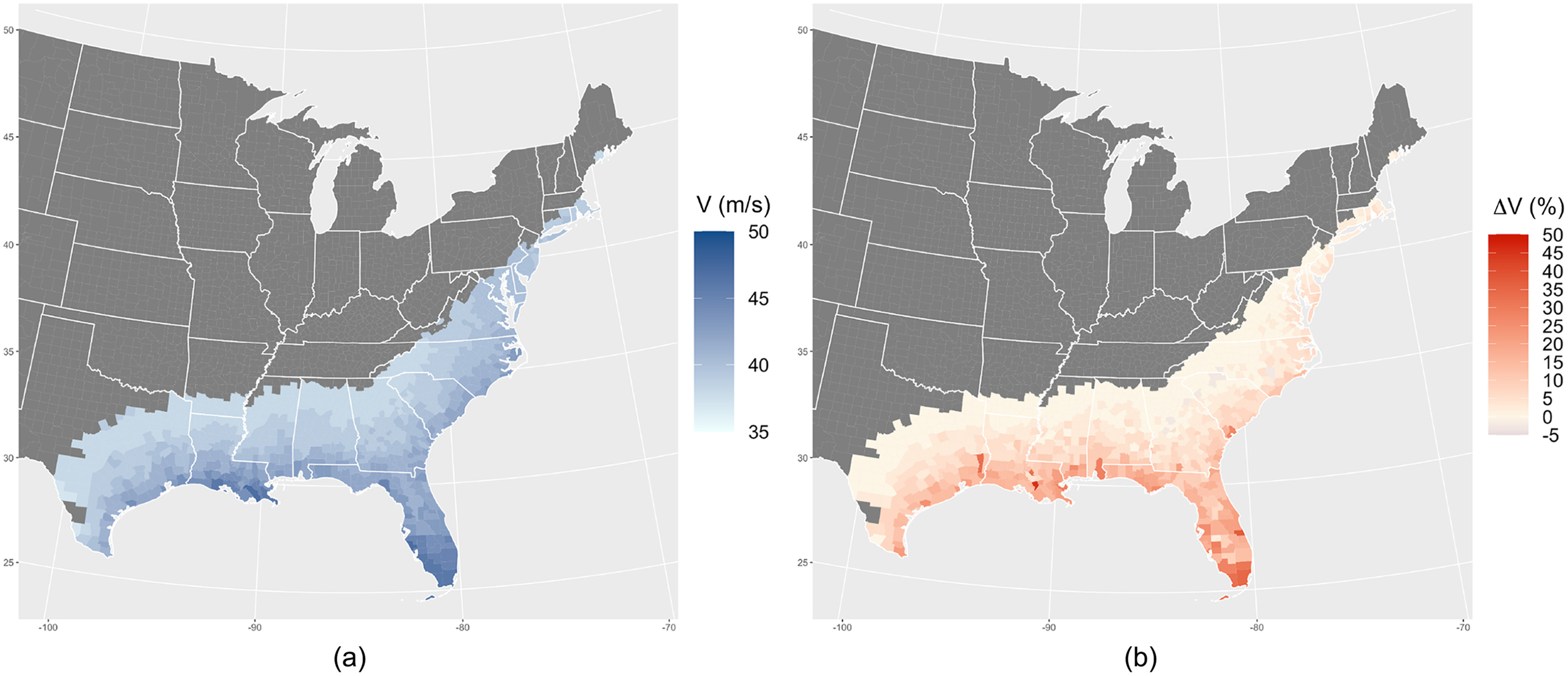
As an initial effort to understand the changes in the extreme wind speed distributions in the United States due to climate change, the 50-year MRI wind speeds were calculated for the years 2000 and 2050. Fig. 2 shows the estimated 50-year wind speed in 2000 and the percent increase in the 50-year wind speed by the year 2050. The 50-year wind speeds in 2000 increased with proximity to coast and decreased with latitude, and coastal and lower latitude locations also saw the largest percent increases in 50-year wind speeds by 2050. There was an average increase of 4.6% overall and 10.0% along the coast, with numerous locations along the Gulf and South Atlantic coasts experiencing increases of 25%–40%. Inland locations generally experienced little or no change in the 50-year wind speed between 2000 and 2050.

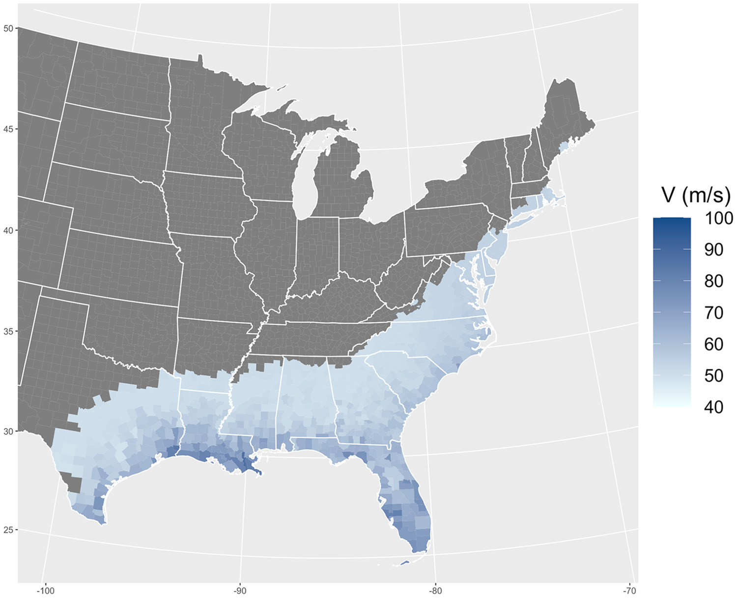
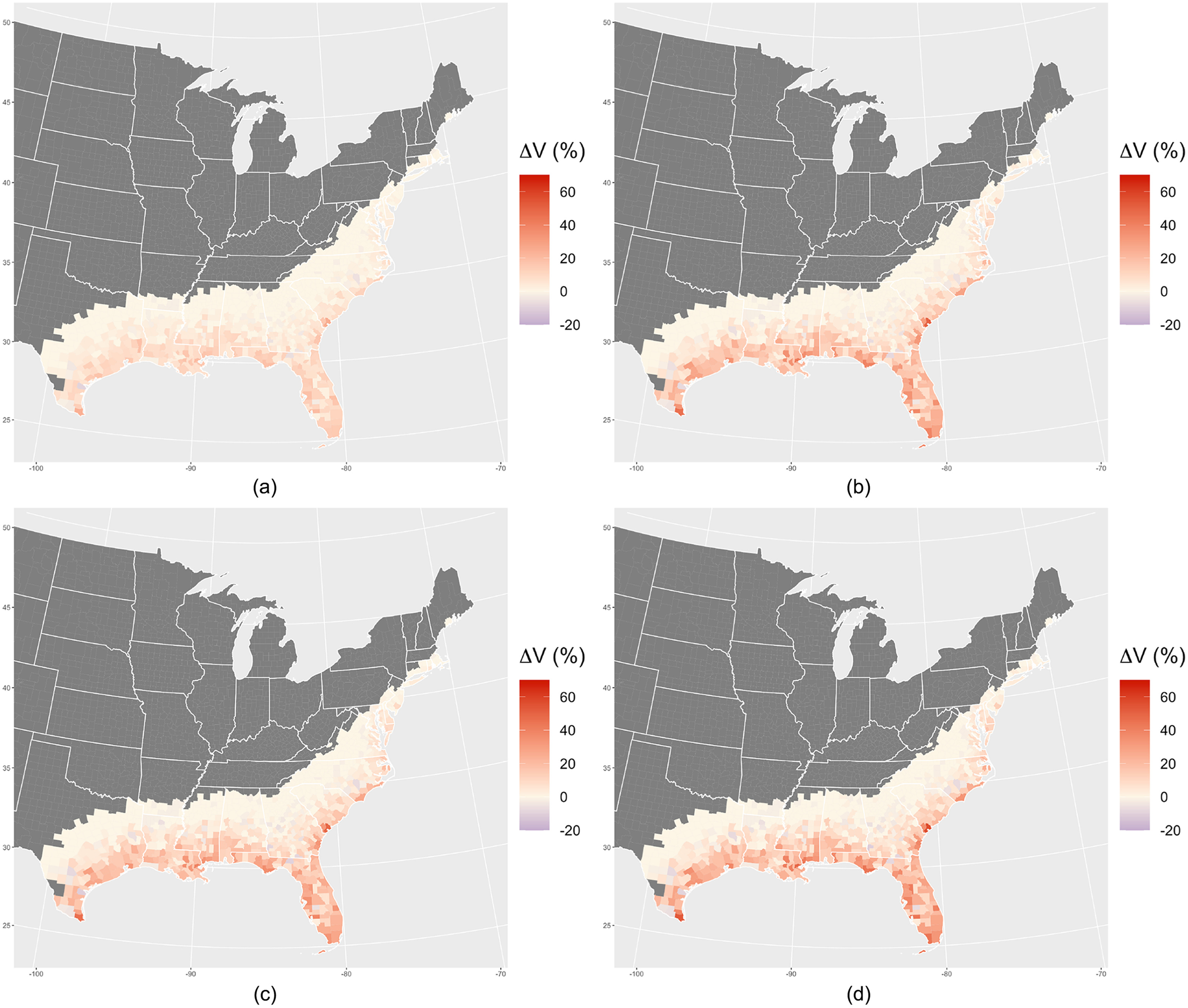
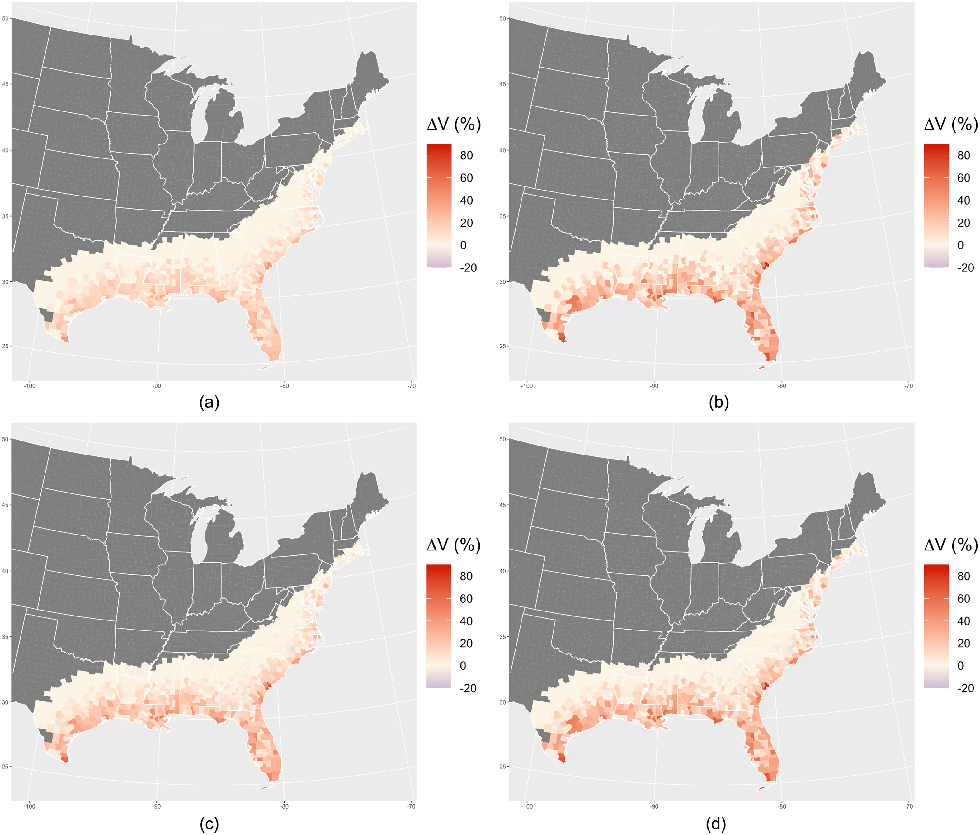
Fig. 3 shows the Risk Category III design wind speeds based on the stationary climate assumption (i.e., 1,700-year winds), and Fig. 4 shows the percent increase in the Risk Category III design wind speed if climate change is accounted for using the LEP-based approach. Figs. S2–S4 show the stationary design wind speeds for Risk Categories I, II, and IV (i.e., 300-year, 700-year, and 3,000-year winds), respectively, and Figs. S5–S7 show the increase in design wind speeds for those risk categories, respectively. Table 3 provides the average percent increase for each risk category.

The largest stationary Risk Category III design wind speeds nearly reach $90\mathrm{m}/\mathrm{s}$ and occur primarily in Florida and Louisiana. The design wind speeds increase with proximity to the coast and decrease with latitude. The percent increases in Risk Category III design wind speeds follow a similar geospatial pattern as the stationary design wind speeds, with the largest increases occurring primarily in Florida and Louisiana, and the magnitude of the increases in design wind speeds increasing with proximity to the coast while decreasing with latitude. The largest Risk Category III design wind speed increases are around 50%, but as mentioned in the “Comparison with ASCE 7-22” section, the results for individual counties should be interpreted with caution. Still, large swathes of the Gulf and South Atlantic coasts see consistent increases of 30%–40%, depending on the year of construction and design lifetime, with a later year of construction and a longer design lifetime being correlated with larger increases [Fig. 4(d)].

The trends in the Risk Category III data hold for the other risk categories. For each risk category, the stationary design wind speeds generally increased with proximity to coast and lower latitude. Additionally, the percentage increase in design wind speeds also generally increased with proximity to coast, lower latitude, a later build year, and a longer design lifetime. Depending on the combination of risk category, build year, and design lifetime, the mean design wind speeds across all counties studied increased by 3%–6% (Table 3). Structures built in 2000 with a 50-year lifespan (Existing Structures–Average Lifespan scenario) experienced the lowest average percentage increase while structures built in 2030 with a lifespan of 70 years (Planned Structures–Longer Lifespan scenario) experienced the highest average percentage increase. When only coastal locations as defined by USCB (2018) were considered, the average percentage increases increased to 6%–15% (Table 3). It is also worth noting that those numbers are only average increases; many locations along the Gulf coast consistently saw increases of 30%–40% as seen in Figs. 4 and S5–S7.

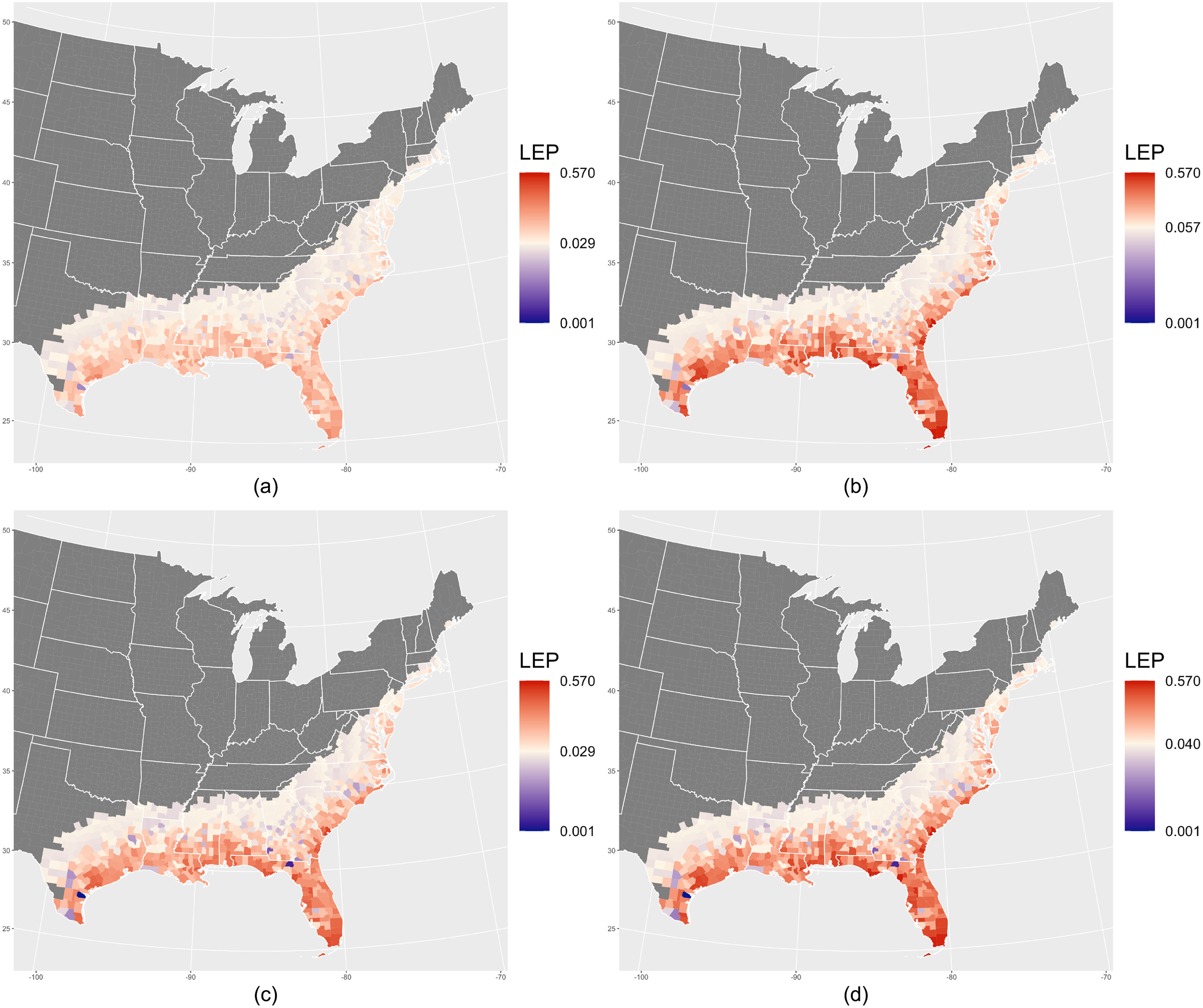
The resulting LEPs if the stationary design wind speeds were used in the changing climate were calculated. Fig. 5 shows the resulting LEPs for each county in the study for Risk Category III. Figs. S8–S10 show the resulting LEP values for Risk Category I, II, and IV structures, respectively. The target LEP, and the minimum and maximum resulting LEPs, are labeled on the color bars in the figures. In some instances, the resulting LEPs were less than 0.001, but the lower bound of the color bar was limited to 0.001 for clarity. Like the increases in design wind speeds, the exceedance of the resulting LEPs over the target value for Risk Category III structures increased with proximity to the coast, year of construction, and design lifetime, while they decreased with latitude. While the target LEP for Risk Category III is 0.04, the resulting LEPs exceeded 0.40 for many locations along the Gulf Coast, notably South Florida, especially for later year of construction and longer design lifetime [Fig. 5(d)], and this is equivalent to at least a 40% chance of exceedance over a structure’s lifetime. The trends in resulting LEPs were consistent across all risk categories.

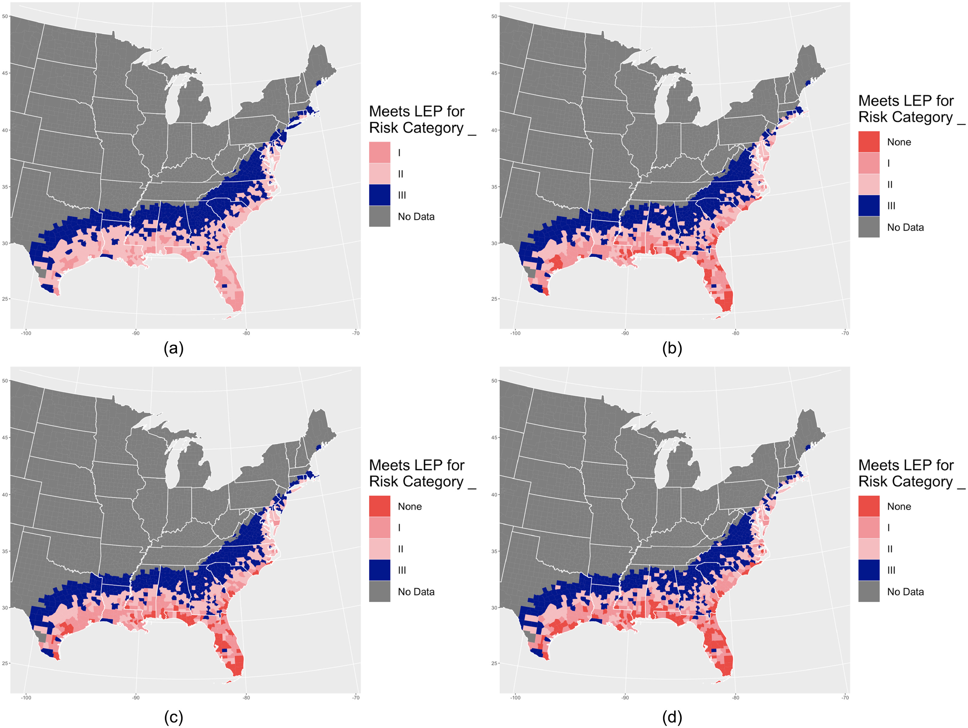
Based on the resulting LEPs, it was possible to determine the effective risk category a structure would be built to if it was designed using the stationary assumption. For example, the allowable LEPs for Risk Category II and III structures are 0.069 and 0.029, respectively, assuming a 50-year service lifetime. If a Risk Category III structure had an LEP of 0.04, it would experience failure rates consistent with Risk Category II structures and would effectively be designed as a Risk Category II structure. Fig. 6 shows the effective risk category for Risk Category III structures. Figs. S11–S13 show the effective risk category for Risk Category I, II, and IV structures, respectively. Table 4 then highlights the proportion of counties that fail to meet their target LEP and are thus at least one effective risk category too low. Because even a small increase in resulting LEP is enough to cause a decrease in effective risk category, Table 5 gives the proportion of counties that have design wind speeds which are at least two risk categories too low, reflecting more substantial increases in risk.

For Risk Category III structures, it appears that structures at least approximately 300 km inland are relatively unaffected by changes in TC winds, as we focused on wind effects within 200 km of the center of the storm. The most significant change is that structures closer to the coast fall further short of their LEP targets. For example, many of the Risk Category III structures in South Florida built in 2000 with a design lifetime of 50 years (Existing Structures–Average Lifespan scenario) would be functionally designed as Risk Category I or II, but most structures in that area built in 2030 with a design lifetime of 70 years (Planned Structures–Longer Lifespan scenario) would fail to even meet the Risk Category I LEPs. Considering the entire study area, 26% of Risk Category III structures under the Planned Structures–Longer Lifespan scenario would meet Risk Category II requirements, a further 17% would meet only Risk Category I requirements, and an additional 10% would fail to meet the target LEPs for any risk category. If only coastal locations are considered, those numbers rise to 33%, 24%, and 30%, respectively.

For all risk categories, the percentage of structures failing to meet the required LEP increased with design lifetime and year of construction. The percentage of structures failing to meet the required LEP fell slightly for higher risk categories, but regardless of the risk category, a significant percentage of structures fell short of the requirements. Depending on the risk category, design lifetime, and year of construction, 43%–57% of the overall counties studied and 71%–89% of coastal counties had stationary design wind speeds that would not yield acceptable LEPs in the changing climate (Table 4). Additionally, numerous locations fell far short of the LEP requirements. For Risk Categories II–IV, depending on the design lifetime and year of construction, 8%–36% of all counties studied experienced LEPs that were at least two risk categories too low, and those numbers increased to 25%–66% for coastal counties (Table 5). For example, in up to 26% of all counties studied and 54% of coastal counties, a Risk Category III structure would be effectively designed as Risk Category I or lower.

As mentioned earlier, the LEP-based approach (targeting the LEP for each risk category specified by ASCE 7-22) may lead to annual failure rates that exceed those currently specified by ASCE 7-22 toward the end of the design lifetime. It is possible to yield acceptable annual levels of risk by using an MRI-based approach based on the most extreme year in a structure’s lifetime, although this is a more conservative approach. Because MRIs and LEPs are equivalent measures of risk in a stationary climate, it was not necessary to recalculate the stationary design wind speeds (Figs. 3 and S2–S4) for this approach. The nonstationary MRI design wind speeds were calculated for the design lifetimes and construction years specified in Table 1. Because the GPD parameters were linearly interpolated in this study, the most extreme year always occurred at the beginning or end of a structure’s lifetime, usually the latter since most locations experienced increases in wind speeds over time under climate change.

Fig. 7 shows the increases in the design wind speeds for Risk Category III using the MRI-based approach, while Figs. S14–S16 show the percent increases in design wind speed using the MRI-based approach for Risk Categories I, II, and IV. The trends for increases in Risk Category III design wind speeds using the MRI-based approach are similar to those using the LEP-based approach, with the largest increases occurring primarily in Florida and Louisiana, and the magnitude of the increases increasing with proximity to the coast while decreasing with latitude. Many locations along the Gulf and South Atlantic coasts saw increases of up to 50% (depending on the year of construction and design lifetime), which is larger than the 40% increases seen with the LEP-based approach.

Depending on the combination of risk category, build year, and design lifetime, the mean design wind speeds using the MRI-based approach increased by 5%–10%, and this increased to 11%–25% when only considering coastal locations. As expected, the MRI-based approach leads to higher design wind speeds. The MRI-based approach is also more prone to outliers, as only the most extreme year of data is considered, whereas every year of a structure’s lifetime is considered in the LEP-based method. If the MRI-based approach is used in the nonstationary climate, it may be necessary to run a larger simulation to reduce this propensity for outliers. The MRI-based approach also does not yield as many decreases in design wind speed as the LEP-based approach, as it considers only the worst-case year. The only reason it yields decreases at all is because for counties with decreasing wind speeds, the highest extreme wind speeds for the two design scenarios built in 2030 are in 2030, and those are less than the extreme wind speeds in 2000 calculated for the stationary approach.

While no previous studies have calculated design wind speeds for the United States using the LEP method, previous studies have done so using the MRI-based approach. Esmaeili and Barbato (2021) found that the design wind speeds associated with the MRIs provided by ASCE 7-22 increased on the coast by an average of approximately 25% for all risk categories under the emissions scenario RCP8.5 by the year 2060. None of the scenarios in this paper have design lifetimes that end in 2060, but there were scenarios with a 50-year service lifetime ending in 2050 and 2080, which saw average increases in the MRI-based design wind speed on the coast of around 11% and 17%, respectively [Figs. 7(a and c) and S14–16(a and c)]. The magnitude of those increases is comparable to those of Esmaeili and Barbato (2021), and the slightly lower values in this study can be largely attributed to different predictions about the Northeastern United States, an area which warrants further discussion.

There are many conflicting predictions about both the magnitude and geospatial distribution of increases in design wind speed in the Northeastern United States due to climate change. Esmaeili and Barbato (2021) predicted the highest increases in design winds to occur in the Northeast, on the order of 30%–40%, with the largest values occurring in Massachusetts, the northernmost point considered. Snaiki and Wu (2020a) found that for Risk Category I–III structures, the range of design wind speed increases along the Northeastern coast was 0%–15% under RCP8.5 in the future climate of 2081–2100. The largest increases occurred along the Delmarva Peninsula and the coast of Maine, and the increases converged to around 0% near Cape Cod. Mudd et al. (2014) found that Risk Category II design wind speeds increased the most in Maine, around 25%, with the rest of the Northeast coast experiencing a relatively uniform increase of around 10%. Finally, this study found design wind speeds for Risk Category I–III structures increased around 20%–30% along the Delmarva Peninsula and around 0%–20% in New England, although there were few locations studied there (Figs. 7 and S14–15). Some of the discrepancies can be explained by differences in TC modeling and study parameters; although all four studies assumed RCP8.5, each study calculated the results for different years ranging between 2060–2100 and used different TC models. Also, this study employed a synthetic data set that is limited in sample size (1,000–1,500-year simulations) and has large statistical uncertainty for the Northeast region. Still, the significant variation in the geospatial distribution of increases suggests fundamental research is needed for this region (e.g., on the effect of ET, which is not explicitly considered in the synthetic TC models).

The results suggest that increased TC activity due to climate change renders the current ASCE 7 design wind speeds unconservative in many locations, but there are several aspects of this study which require further research. The synthetic TC data from Gori et al. (2022) featured an increase in TC frequency due to climate change, which is supported by some recent studies (Bhatia et al. 2018; Emanuel 2021; Fedorov et al. 2018; Vecchi et al. 2019), but other studies suggest that TC frequency will either remain the same or decrease (Committee on Adaption to a Changing Climate 2018; Knutson et al. 2020). Gori et al. (2022) found that even if the TC frequency was held constant, the joint surge-rainfall hazard (driven by the wind) was still projected to increase greatly with climate change, suggesting that a decrease in TC frequency does not preclude an increase in extreme wind speeds. Still, further research is needed to establish the effects of climate change on TC frequency and thus on the design wind speeds.

In this study, some inland counties and a few Gulf Coast counties, specifically Nueces County, TX and Cameron Parish, LA, experienced decreases in design wind speed. It is physically unlikely for the counties along the Gulf Coast to experience decreases in design wind speed with climate change, especially given that their bordering counties experienced increases in design wind speed (Fig. 4) and that the counties themselves experienced increases in 50-year wind speeds (Fig. 2). Even with the large number of synthetic TCs (1,000–1,500 years of simulations) from Gori et al. (2022), there was still a large degree of uncertainty in the return level curves at the long return periods (e.g., 3,000-year winds). It is likely the apparent decreases in design wind speeds are mainly due to statistical uncertainty, and future research should use a much greater number of synthetic TCs to reduce uncertainty. The location sampling density could also be increased, perhaps calculating wind speeds for each zip code as done in Mudd et al. (2014), allowing for smoothing of the design wind speeds and the exclusion of statistical outliers. Given the large geophysical regions covered and relatively large number of simulations considered, simple parametric wind models were applied in this study; boundary layer models (e.g., Vickery et al. 2009a) may also be used to obtain more accurate surface wind speeds in future studies.

The differences in the projection of design wind speeds in this study and in previous studies result mainly from the different TC models used. While the model used in this study considers the effect of various nonstationary climate variables, most other models used in the previous studies considered only the effect of SST change. SST change is a primary driver of increased TC intensity from climate change, but additional changes in climate may either compound or diminish the effects of that increased intensity on the design wind speeds in the contiguous United States. For example, changes in large-scale wind patterns may influence the landfalling rate of TCs at various points along the coast. In addition to the synthetic TC models of Emanuel et al. (2008) and Snaiki and Wu (2020b), those of Jing and Lin (2019, 2020) and Lee et al. (2018) also involve various key climate variables and can be used to efficiently simulate synthetic TCs for future climates. The methodology to calculate design wind speeds presented here does not depend on the choice of synthetic model and can thus be easily adapted as synthetic TC modeling advances. Finally, uncertainties induced by the TC modeling may be better quantified by calculating the design wind speeds using various TC models.

Yeo et al. (2014) found that the coastal locations they studied in the Southeast United States had extreme wind curves dominated by TCs, so it is unlikely that increases in non-TC winds due to climate change would impact those locations significantly. However, inland extreme winds are often dominated by thunderstorm winds (Twisdale and Vickery 1992), and extreme winds for the coastal midlatitudes are highly influenced by ETCs (Colle et al. 2015). Thus, further research should be conducted on how climate change will affect thunderstorm and ETC winds, as those could lead to significantly increased wind speeds for the interior United States as well as the mid-Atlantic and Northeast US coasts. Future research should also consider the impacts of climate change on hybrid events, like Hurricane Sandy, as current synthetic TC models do not capture the effect of the ET. It is not clear how hybrid events may change differently compared to TC events under climate change. As with TC-winds, the methodology to calculate design wind speeds does not depend on the underlying non-TC wind distributions and could be adapted to account for nonstationary non-TC winds as the science advances.

Climate nonstationarity presents new challenges for the building code. It has not been decided whether future design wind speeds should be based on maintaining the current lifetime risk (e.g., the LEP-based approach) or on maintaining the current annual risk (e.g., the MRI-based approach). Still, in both approaches, design wind speeds are a function of both structure lifetime and year of construction in addition to the current parameters of location and risk category, making it impractical to include design wind speed maps for all the possible combinations of risk category, lifetime, and build year. In addition to the ASCE 7 design wind speed maps, designers can currently obtain equivalent design wind speeds from the online ASCE 7 Hazard Tool (ASCE 2024), which is likely a more efficient method when considering a nonstationary climate. The wind speed calculations on the website would have to be updated to reflect a nonstationary climate, either via the LEP-based or MRI-based methods; for the user, the only change would be a requirement to specify the design lifetime of the structure and the structure’s year of construction. As an example of what this would entail, a rudimentary R package was created to give the nonstationary design wind speed based on a structure’s location, risk category, lifespan, and year of construction, using either the LEP-based or MRI-based method. This program is available from the authors upon reasonable request.

There are also many policy considerations to be made. As climate models advance and better estimates of greenhouse gas emissions are obtained, design wind speed projections should also be updated. These projections will be highly dependent on our future emissions, and it must be considered how often to update the design wind speeds. This study considered only the high emissions scenario SSP5-8.5, but Xi et al. (2023) found that the moderate emissions scenario SSP2-4.5 still results in significant increases in TC hazards. Various emissions scenarios may be considered in the development of the building code. Additionally, it must be considered how to grandfather in existing structures which may have been designed for lower design wind speeds.

In the meantime, designers may consider performing climate change impact studies on their structures, where the performance of the structure under variable wind conditions can be tailored to the owner’s requirements. The online hazard tool can be used to provide the underlying full hazard information (e.g., annual maximum wind distributions) to support performance-based design that also accounts for the uncertainty in structural resistance. Because velocity pressure is a function of design wind speed squared, the estimated average increase of 6%–15% in design wind speeds on the coast would lead to an average 12%–32% increase in wind pressures. Additionally, given the high spatial variability of the design wind speed increases, portions of the Gulf Coast could see a doubling of their wind pressures due to increased design wind speeds. For those structures that have already been built, designers may wish to perform similar analyses to ensure that the structures will still perform at acceptable risk levels in the changing climate.

References

ASCE. 2021. Minimum design loads and associated criteria for buildings and other structures. Reston, VA: ASCE. https://doi.org/10.1061/9780784415788.
Batts, M. E., M. R. Cordes, L. R. Russell, J. R. Shaver, and E. Simiu. 1980. “Hurricane wind speeds in the United States.” In Building science series 124. Washington, DC: National Bureau of Standards.
Bhatia, K., G. Vecchi, H. Murakami, S. Underwood, and J. Kossin. 2018. “Projected response of tropical cyclone intensity and intensification in a global climate model.” J. Clim. 31 (20): 8281–8303. https://doi.org/10.1175/JCLI-D-17-0898.1.
Buchanan, M. K., R. E. Kopp, M. Oppenheimer, and C. Tebaldi. 2016. “Allowances for evolving coastal flood risk under uncertain local sea-level rise.” Clim. Change 137 (3): 347–362. https://doi.org/10.1007/s10584-016-1664-7.
Colle, B. A., J. F. Booth, and E. K. M. Chang. 2015. “A review of historical and future changes of extratropical cyclones and associated impacts along the US East coast.” Curr. Clim. Change Rep. 1 (3): 125–143. https://doi.org/10.1007/s40641-015-0013-7.
Committee on Adaption to a Changing Climate. 2018. Climate resilient infrastructure: Adaptive design and risk management. Reston, VA: ASCE. https://doi.org/10.1061/9780784415191.
Cui, W., and L. Caracoglia. 2016. “Exploring hurricane wind speed along US Atlantic coast in warming climate and effects on predictions of structural damage and intervention costs.” Eng. Struct. 122 (Apr): 209–225. https://doi.org/10.1016/j.engstruct.2016.05.003.
Das, S., D. Zhu, and Y. Yin. 2020. “Comparison of mapping approaches for estimating extreme precipitation of any return period at ungauged locations.” Stochastic Environ. Res. Risk Assess. 34 (8): 1175–1196. https://doi.org/10.1007/s00477-020-01828-7.
Davenport, A. G., C. S. B. Grimmond, T. R. Oke, and J. Wieringa. 2000. “Estimating the roughness of cities and sheltered country.” In Proc., 12th Conf. on Applied Climatology, 96–99. Boston: American Meteorological Society.
Ellingwood, B. R., and J. Y. Lee. 2016. “Life cycle performance goals for civil infrastructure: Intergenerational risk-informed decisions.” Struct. Infrastruct. Eng. 12 (7): 822–829. https://doi.org/10.1080/15732479.2015.1064966.
Emanuel, K. 2017. “Assessing the present and future probability of Hurricane Harvey’s rainfall.” Proc. Natl. Acad. Sci. 114 (48): 12681–12684. https://doi.org/10.1073/pnas.1716222114.
Emanuel, K. 2021. “Response of global tropical cyclone activity to increasing CO2: Results from downscaling CMIP6 models.” J. Clim. 34 (1): 57–70. https://doi.org/10.1175/JCLI-D-20-0367.1.
Emanuel, K., S. Ravela, E. Vivant, and C. Risi. 2006. “A statistical deterministic approach to Hurricane risk assessment.” Bull. Am. Meteorol. Soc. 87 (3): S1–S5. https://doi.org/10.1175/BAMS-87-3-Emanuel.
Emanuel, K., R. Sundararajan, and J. Williams. 2008. “Hurricanes and global warming: Results from downscaling IPCC AR4 simulations.” Bull. Am. Meteorol. Soc. 89 (3): 347–368. https://doi.org/10.1175/BAMS-89-3-347.
Esmaeili, M., and M. Barbato. 2021. “Predictive model for hurricane wind hazard under changing climate conditions.” Nat. Hazard. Rev. 22 (3): 04021011. https://doi.org/10.1061/(ASCE)NH.1527-6996.0000458.
Fedorov, A. V., L. Muir, W. R. Boos, and J. Studholme. 2018. “Tropical cyclogenesis in warm climates simulated by a cloud-system resolving model.” Clim. Dyn. 52 (Feb): 107–127. https://doi.org/10.1007/s00382-018-4134-2.
Gori, A., N. Lin, D. Xi, and K. Emanuel. 2022. “Tropical cyclone climatology change greatly exacerbates US extreme rainfall-surge hazard.” Nat. Clim. Change 12 (2): 171–178. https://doi.org/10.1038/s41558-021-01272-7.
Hallegatte, S. 2007. “The use of synthetic hurricane tracks in risk analysis and climate change damage assessment.” J. Appl. Meteorol. Climatol. 46 (11): 1956–1966. https://doi.org/10.1175/2007JAMC1532.1.
Hunter, J. 2012. “A simple technique for estimating an allowance for uncertain sea-level rise.” Clim. Change 113 (2): 239–252. https://doi.org/10.1007/s10584-011-0332-1.
Jing, R., and N. Lin. 2019. “Tropical cyclone intensity evolution modeled as a dependent hidden Markov process.” J. Clim. 32 (22): 7837–7855. https://doi.org/10.1175/JCLI-D-19-0027.1.
Lee, C.-Y., M. K. Tippett, A. H. Sobel, and S. J. Camargo. 2018. “An environmentally forced tropical cyclone hazard model.” J. Adv. Model. Earth Syst. 10 (1): 223–241. https://doi.org/10.1002/2017MS001186.
Lin, N., and D. Chavas. 2012. “On hurricane parametric wind and applications in storm surge modeling.” J. Geophys. Res. 97 (D9): 1–19. https://doi.org/10.1029/92JD00846.
Lin, N., K. A. Emanuel, J. A. Smith, and E. Vanmarcke. 2010. “Risk assessment of hurricane storm surge for New York City.” J. Geophys. Res.: Atmos. 115 (D18): 1–11. https://doi.org/10.1029/2009JD013630.
Lin, N., P. Lane, K. A. Emanuel, R. M. Sullivan, and J. P. Donnelly. 2014. “Heightened hurricane surge risk in northwest Florida revealed from climatological-hydrodynamic modeling and paleorecord reconstruction.” J. Geophys. Res.: Atmos. 119 (14): 8606–8623. https://doi.org/10.1002/2014JD021584.
Lin, N., R. Marsooli, and B. Colle. 2019. “Storm surge return levels induced by the mid-to-late-twenty-first-century extratropical cyclones in the Northeastern United States.” Clim. Change 154 (1–2): 143–158. https://doi.org/10.1007/s10584-019-02431-8.
Lombardo, F. T., J. A. Main, and E. Simiu. 2009. “Automated extraction and classification of thunderstorm and non-thunderstorm wind data for extreme-value analysis.” J. Wind Eng. Ind. Aerodyn. 97 (3–4): 120–131. https://doi.org/10.1016/j.jweia.2009.03.001.
Marsooli, R., N. Lin, K. Emanuel, and K. Feng. 2019. “Climate change exacerbates hurricane flood hazards along US Atlantic and Gulf Coasts in spatially varying patterns.” Nat. Commun. 10 (1): 3785. https://doi.org/10.1038/s41467-019-11755-z.
Mudd, L., Y. Wang, C. Letchford, and D. Rosowsky. 2014. “Hurricane wind hazard assessment for a rapidly warming climate scenario.” J. Wind Eng. Ind. Aerodyn. 133 (Aug): 242–249. https://doi.org/10.1016/j.jweia.2014.07.005.
Pintar, A. L., E. Simiu, F. T. Lombardo, and M. Levitan. 2015. Maps of non-hurricane nontornadic wind speeds with specified mean recurrence intervals for the contiguous United States using a two-dimensional Poisson process extreme value model and local regression. Gaithersburg, MD: NIST. https://doi.org/10.6028/NIST.SP.500-301.
Rootzén, H., and R. W. Katz. 2013. “Design life level: Quantifying risk in a changing climate: Design life level.” Water Resour. Res. 49 (9): 5964–5972. https://doi.org/10.1002/wrcr.20425.
Seeley, J. T., and D. M. Romps. 2015. “The effect of global warming on severe thunderstorms in the United States.” J. Clim. 28 (6): 2443–2458. https://doi.org/10.1175/JCLI-D-14-00382.1.
Snaiki, R., and T. Wu. 2020a. “Hurricane hazard assessment along the United States Northeastern coast: Surface wind and rain fields under changing climate.” Front. Built Environ. 6 (Oct): 573054. https://doi.org/10.3389/fbuil.2020.573054.
Task Committee on Future Weather and Climate Extremes. 2021. Impacts of future weather and climate extremes on United States infrastructure. Reston, VA: ASCE. https://doi.org/10.1061/9780784415863.
Trapp, R. J. 2021. “Potential effects of anthropogenic climate change on non-synoptic wind storm hazards.” In The Oxford handbook of non-synoptic wind storms, edited by H. Hangan and A. Kareem. Oxford, UK: Oxford University Press. https://doi.org/10.1093/oxfordhb/9780190670252.013.4.
Twisdale, L. A., and P. J. Vickery. 1992. “Research on thunderstorm wind design parameters.” J. Wind Eng. Ind. Aerodyn. 41 (1–3): 545–556. https://doi.org/10.1016/0167-6105(92)90461-I.
Vecchi, G. A., et al. 2019. “Tropical cyclone sensitivities to CO2 doubling: Roles of atmospheric resolution, synoptic variability and background climate changes.” Clim. Dyn. 53 (9–10): 5999–6033. https://doi.org/10.1007/s00382-019-04913-y.
Vickery, P. J., D. Wadhera, M. D. Powell, and Y. Chen. 2009a. “A hurricane boundary layer and wind field model for use in engineering applications.” J. Appl. Meteorol. Climatol. 48 (2): 381–405. https://doi.org/10.1175/2008JAMC1841.1.
Villarini, G., and J. A. Smith. 2010. “Flood peak distributions for the eastern United States.” Water Resour. Res. 46 (6): 1–17. https://doi.org/10.1029/2009WR008395.
Villarini, G., J. A. Smith, M. L. Baeck, R. Vitolo, D. B. Stephenson, and W. F. Krajewski. 2011. “On the frequency of heavy rainfall for the Midwest of the United States.” J. Hydrol. 400 (1–2): 103–120. https://doi.org/10.1016/j.jhydrol.2011.01.027.
Walsh, K. J. E., S. J. Camargo, T. R. Knutson, J. Kossin, T.-C. Lee, H. Murakami, and C. Patricola. 2019. “Tropical cyclones and climate change.” Trop. Cyclone Res. Rev. 8 (4): 240–250. https://doi.org/10.1016/j.tcrr.2020.01.004.
Xi, D., N. Lin, and A. Gori. 2023. “Increasing sequential tropical cyclone hazards along the US east and Gulf Coasts.” Nat. Clim. Change 13 (3): 258–265. https://doi.org/10.1038/s41558-023-01595-7.
Xu, H., N. Lin, M. Huang, and W. Lou. 2020. “Design tropical cyclone wind speed when considering climate change.” J. Struct. Eng. 146 (5): 04020063. https://doi.org/10.1061/(ASCE)ST.1943-541X.0002585.
Yeo, D. H., N. Lin, and E. Simiu. 2014. “Estimation of hurricane wind speed probabilities: Application to New York City and other coastal locations.” J. Struct. Eng. 140 (6): 04014017. https://doi.org/10.1061/(ASCE)ST.1943-541X.0000892.
If you have the appropriate software installed, you can download article citation data to the citation manager of your choice. Simply select your manager software from the list below and click Download.