A Statistical Principal Component Regression-Based Approach to Modeling the Degradative Effects of Local Climate and Traffic on Airfield Pavement Performance
Publication: Journal of Transportation Engineering, Part B: Pavements
Volume 148, Issue 2
Abstract
Airfield pavement systems support the global economy, passenger travel, and national defense. Accurate pavement degradation predictions are critical inputs for maintenance and repair decisions, and when skillful, they may reduce the need for time-intensive, costly physical inspections that disrupt airfield operations. Existing airport pavement management systems (APMS) compute expected degradation as a function of pavement type and age, but they do not account for local climate and traffic conditions and they are not built to adapt to future changes in either mode of variability. This paper implements a bias-reduced statistical model that reveals the effects of local conditions using observed historical climatic and aircraft traffic data. Model performance is evaluated using a diverse data set from nine Air Force installations, encompassing three major Köppen-Geiger climate zones in the contiguous United States and representing a wide range of aircraft. Environmental factors are more impactful on pavement degradation than aircraft traffic; a climate-only model produces values as high as 0.84, while traffic improves explained variance across installations ( = 0.86–0.97) for the most heavily trafficked pavement family. This work illustrates the impactful role of climate in pavement degradation and demands implementation into the current APMS. Airfield asset managers can use this adaptable framework to more accurately determine sources of local degradation and inform sustainable pavement design and management practices.
Introduction
Airfield pavements support the global economy, passenger travel, and national defense. Since condition assessments disrupt airfield operations, accurate predictions of degradation are essential to rehabilitation planning and reduce the need for time-intensive, costly physical inspections (Mulry et al. 2015). Data-driven pavement degradation models, such as airport pavement management systems (APMS), predict future pavement conditions using historical observations and are essential tools to plan pavement rehabilitation interventions between physical inspections (Gendreau and Soriano 1998; Shahin 2005). Despite the successful, widespread use of APMS (Ismail et al. 2009), their applicability is limited by the number and types of variables used to drive predictions and the fact that they lack local calibration. As such, APMSs cannot adapt to likely future conditions, such as nonstationary climate or changes in use patterns.
Research studies investigating airfield pavement asset management have focused on two main areas: (1) sources of pavement deterioration and manifestations of damage types; and (2) modeling approaches and methods to predict future pavement conditions and encourage sustainable pavement life-cycle assessment practices. The first area of study discusses the most prevalent causes for distress on rigid and flexible airfield surfaces, such as age, environment, traffic, maintenance history, and construction quality (Haas 2001). Active contributions to pavement deterioration fall broadly into climate exposure and use. Consequently, the unique effects of temperature and precipitation (Chinowsky et al. 2013), soil conditions (Ankit et al. 2011), aircraft loading (Ameri et al. 2011; Sawant 2009), pass frequency (White et al. 1997), and tire configuration (Shafabakhsh and Kashi 2015; Wang and Al-Qadi 2011) introduce complexity in pavement degradation. Most model-based approaches are univariate, attempting to isolate the degradative influence of a single independent variable. While this method of analysis is useful, as it eliminates risk stemming from multicollinearity, it ignores the reality that multiple independent variables likely influence pavement condition. A second issue is that the resolution of distress data used to inform models often lacks the spatial and temporal resolution required to produce reliable predictions for specific locations. Lastly, modeling attempts have failed to account for climate’s role due to the lack of spatial granularity necessary to incorporate high-resolution climatic data (Sahagun et al. 2017).
Researchers often amalgamate pavement distress and condition data into familial categories, organized by climate zones (Meihaus 2013; Parsons and Pullen 2016) or geographic area (Sahagun et al. 2017), to investigate spatial trends on a larger, e.g., regional scale. Age and remaining service life are commonly used modeling variables that attempt to account for various degradative effects. Still, pavement structure (Ankit et al. 2011), temperature extremes, and precipitation (Bennett 2019) warrant further research to determine whether changing climate could strengthen the relationship between condition and exogenous, stochastic factors. Harvey et al. (2016) suggest a sustainability-minded approach to pavement management under climate change, one that considers the environmental, social, and economic impacts of pavement maintenance practices on future generations. Climate change projections display an expected global temperature change (GTC) of 2.7°C (Kjellstrom et al. 2018; Van Vuuren et al. 2011), which will drive sustainable pavement management practices research. Rigid pavements may experience increased carbonation rates with minimal effects on compressive strength (Kaewunruen et al. 2018) while flexible pavement degradation is expected to increase significantly due to rutting and cracking from more extreme temperature fluctuations (Chinowsky et al. 2013).
The second area of study investigates modeling approaches and methods to predict future pavement conditions. The pavement research community has long recognized the need for data-driven, reliability-based strategies to effectively manage pavement life cycles (Frangopol et al. 2001). However, few APMSs are capable of generating accurate predictions (Ismail et al. 2009). The AIRfield Pavement Consultant System (AIRPACS) is a prototype, heuristic tool that recommends rehabilitation options (Seiler et al. 1991) but lacks robustness and commercial implementation. PAVER is the leading APMS used by the US Department of Defense (DoD) and Federal Aviation Administration (FAA 2014; Shahin and Rozanski 1978).
PAVER is a database, planning tool, and modeling system. It uses a maximum term polynomial regression approach to approximate future pavement conditions for user-defined, like-type pavement families (Shahin 1994; Shahin and Rozanski 1978). Families are typically selected using material type, priority, and use criteria (Shahin 1994). Condition is quantified in PAVER by the Pavement Condition Index (PCI), which is determined through visual inspection from pavement experts guided by validated specifications (ASTM 2012; Shahin 2005; Shahin et al. 1987). Other systems use the International Roughness Index (IRI) (Taylor and Philp 2015) to quantify the need for maintenance and repair. PCI and IRI provide standardized metrics representative of the current health of a pavement section’s surface through subgrade and are useful to compare and model future condition changes (Chih-Yuan and Durango-Cohen 2008; Greene et al. 2004).
Pavement design engineers also use tools such as PCASE (US DoD), FAARFIELD (FAA), and Alize-Airfield (French Aviation Authority) to assist in meeting the unique challenge of creating sustainable pavements subjected to dynamic loads (Adolf 2010; Heymsfield and Tingle 2019). Sustainable transportation practices consider various economic factors, community impacts, and environmental burdens from construction, operations, and end-of-life-cycle decisions (Allen and Albert 2014). Most recognized pavement management systems and design software use deterministic empirical approaches, though other mechanistic and probabilistic models have been used experimentally (Sidess et al. 2021). Moreover, the selection of independent variables is relatively limited for APMS, which mainly considers pavement age despite success in highway modeling systems’ use of other variables (Ismail et al. 2009).
Despite the significant contributions of these studies and modeling systems, little reported research determines the amount of influence from the combined effect of local climate and traffic on airfield pavement degradation. Additionally, no existing APMS is capable of adjusting prediction capability using future condition projections. Accordingly, the objectives of this study are to (1) identify climate and use contributions explaining degradation variation using a framework powered by bias-reduced, principal component regression (PCR) models, and (2) compare a climate-only model with a combined climate and traffic model to determine which category of variables—climate or traffic—is more influential in providing model skill. This approach is expected to have many benefits and address several of the limitations highlighted above.
It is essential for pavement degradation models to use a systems framework that accounts for varying potential conditions such as mission change, new aircraft, or climatic change. Furthermore, the current spectrum of APMS may benefit from understanding the degree to which climate and aircraft traffic contribute individually to pavement degradation, quantified by a negative change in PCI. Climate and use-influenced degradation predictions can be incorporated, where skillful, into the current age-based approach for improved and adaptable modeling of pavement deterioration. Ultimately, having improved accuracy in degradation predictions could lead to more optimized planning of recurring pavement repair actions and drive pavement design engineers to create more intentional mix designs that withstand deterioration sources.
Data
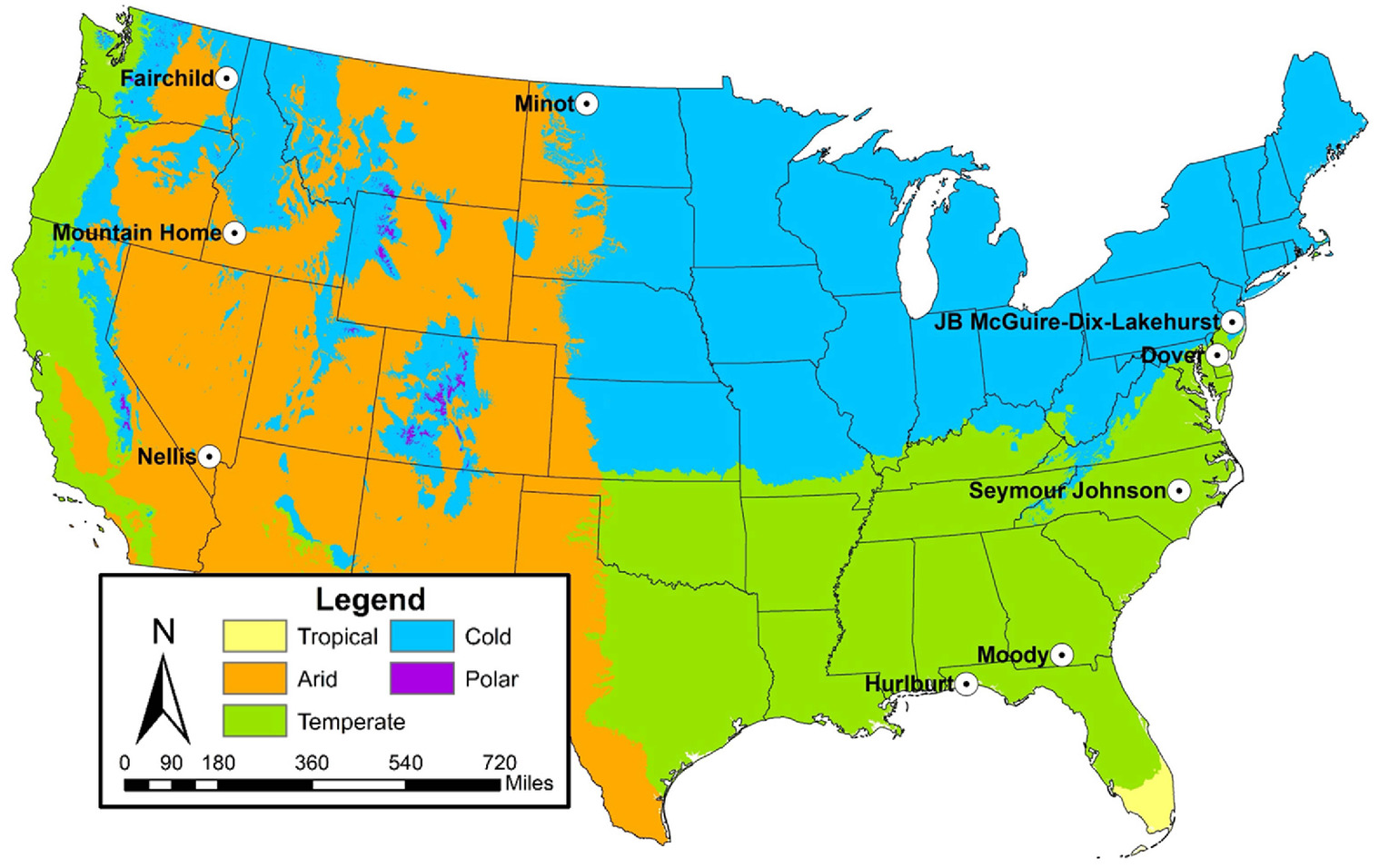
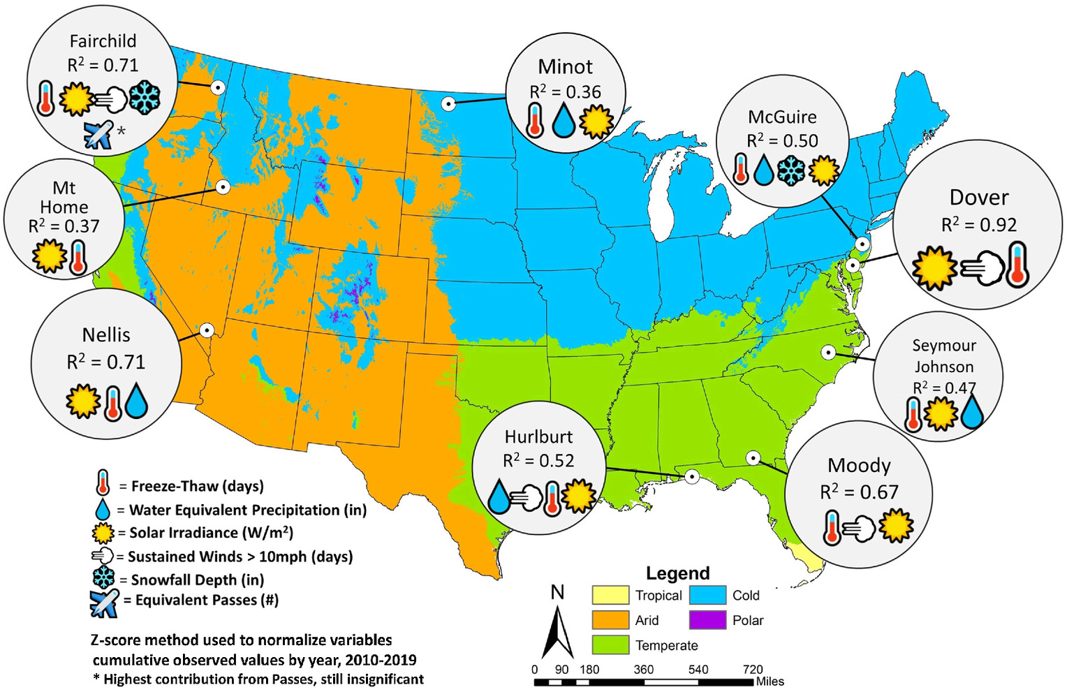
Several location-matched data sets were acquired for pavement type, aircraft traffic, and climate data, with sufficient temporal resolution (daily values that were aggregated into annual time steps) to satisfy the research objectives and produce statistically significant results. The US Air Force (USAF) uses PAVER as its pavement condition database and condition prediction software. This research analyzed PAVER data from nine USAF installations representing pavements from all major, first hierarchy-level Köppen-Geiger climate zones (Delorit et al. 2020) at a 1-km resolution (Beck et al. 2018) and active aircraft types in the contiguous United States, as shown in Fig. 1 and Table 1. These temporally-based zones were chosen for easy identification of installations and to perform further analysis on regional trends.
| Installation | Abbreviation | Nearest city | State | Asset count |
|---|---|---|---|---|
| Dover Air Force Base | Dover | Dover | DE | 60 |
| Fairchild Air Force Base | Fairchild | Spokane | WA | 66 |
| Hurlburt Field | Hurlburt | Fort Walton Beach | FL | 16 |
| McGuire-Dix-Lakehurst, Joint Base | McGuire | Trenton | NJ | 17 |
| Minot Air Force Base | Minot | Minot | ND | 35 |
| Moody Air Force Base | Moody | Valdosta | GA | 17 |
| Mountain Home Air Force Base | MtHome | Mountain Home | ID | 11 |
| Nellis Air Force Base | Nellis | Las Vegas | NV | 11 |
| Seymour Johnson Air Force Base | Seymour John | Goldsboro | NC | 33 |
The Air Force Civil Engineer Center (AFCEC) provided PAVER data summary reports from 2011, 2015, and 2019. The data were filtered to include only viable pavement sections, mainly ensuring homogenous construction of horizontal pavement layers (e.g., no sections with flexible pavement overlaid on a rigid pavement base) and limiting sections that had been altered between inspections during the reporting period, such as through significant rehabilitation. It is assumed that routine maintenance is performed equally across all airfield pavements since that fidelity of information is unavailable. Sahagun et al. (2017) provide a full description of all available data from the AFCEC summary reports to include branch use, section ID, true area, surface type, years since major work, distress description, and condition (PCI).
Aircraft traffic data is recorded by each installation’s air traffic control tower and compiled as an annual Air Traffic Activity Report (ATAR) by the Air Force Flight Standards Agency (AFFSA). The ATAR displays the number of passes per installation, where one pass is counted when an aircraft crosses an imaginary transverse line within 152 m (500 ft) of the end of the runway. This count excludes “touch-and-go” operations where the aircraft never applies its full weight on the pavement surface (UFC 2001b). Within the ATAR, each selected location has a unique total annual pass value. Pass data was available for the years 2010–2019, which, based on the frequency of condition assessments, constrained the analysis to 266 sections between the nine chosen locations. This research converted the aircraft pass data into equivalent passes that account for aircraft type and loading to compare locations. Equivalent pass calculations are discussed in the “Methodology” section. The temporal resolution of each data type had to match for the analysis; the available aircraft traffic data is represented by annual values and was the limiting factor to having finer data resolution for the model application.
Climatic data were procured from AccuWeather’s proprietary database for 2010–2019 from the nearest weather station to each location. The five climatic variables (calculated annually) used in this research are: z-score normalized values for the total count of freeze-thaw (days); sum of daily water equivalent precipitation (in.); sum of daily snowfall (in.); count of days with sustained wind speed above (10 mph) (days); and sum of daily solar irradiance (). These metrics are not exhaustive, but they are representative of variables known to affect built asset performance (Brown 2021). Most notably, air temperature is not directly included as a variable because the effects of air temperature are captured in freeze-thaw and solar irradiance. Some of the selected weather variables, such as freeze-thaw and precipitation, have been limitedly studied in pavements and provided more potential for unique discovery than air temperature, which has been widely studied alone (Qiao et al. 2020; Abed et al. 2019; Li et al. 2013). The impact of solar irradiance and sustained wind on pavements has not been studied but is suspected to contribute to degradation and is included here to promote a more robust analysis.
Methodology
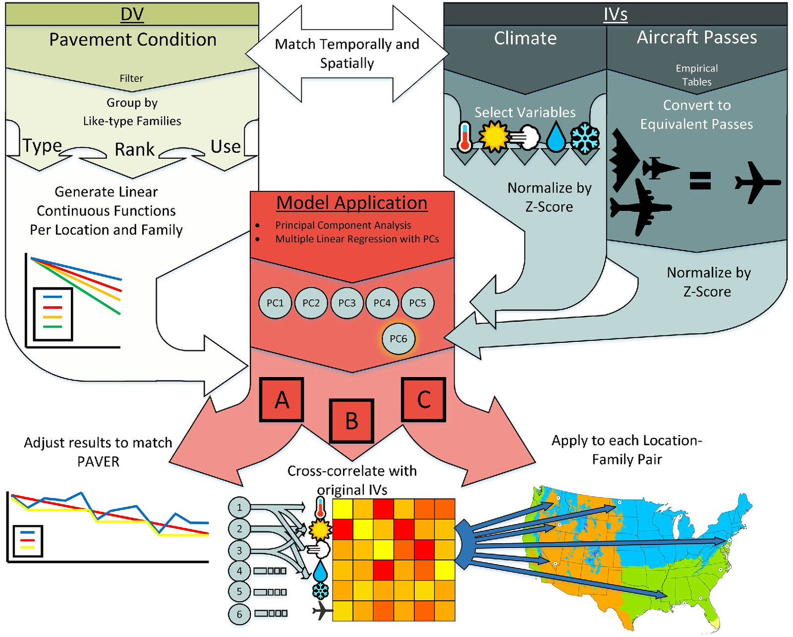
The framework applied to these data sets follows two steps that mimic part of the prediction processes from PAVER to meet the outlined objectives, with a novel model framework application as step three: (1) group families of standardized, like-type pavement sections that share similarities in type and use; (2) produce continuous functions describing degradation for each family-location pair; and (3) execute a cross-validated, PCR model to predict the continuous function using a time series of selected climatic and traffic-based independent variables. The framework is run in two modes—climate only and a combined climate and traffic model (climate-passes)—to create a comparison that enables an analysis of the value of collecting pass data. Fig. 2 is a theoretical framework for this methodology that portrays the data integration into the model.
The first step of this framework follows the standard practice of defining families of like-type pavements. Common criteria used for analysis are pavement type (material/structure), rank (priority), and location on the airfield (use) (Shahin 1994). Table 2 describes the PCASE traffic type designators A through D, which are similar criteria used in pavement design (UFC 2001a). This analysis takes the unique approach of combining the traffic type designators with pavement type. Eight potential families were created. For example, family Rig A captures Portland cement concrete (PCC) pavement sections within the first 304.8 m (1,000 ft) of a runway and primary taxiway surfaces. Rig D and Flex B did not exist in the asset inventory or did not possess sufficient data to perform a statistically significant analysis.
| Pavement type (material/structure) | PCASE traffic type designator |
|---|---|
| Rigid | A |
| Portland cement concrete (PCC) | First 304.8 m (1,000 ft) of runways and primary taxiways |
| Flexible | Designed for full load and channelized traffic |
| Asphalt concrete (AC) | B |
| Asphalt overlaid on AC (AAC) | All aprons |
| Designed for full load and unchannelized traffic | |
| C | |
| Runway interiors and secondary taxiways | |
| Designed for 75% load and unchannelized traffic | |
| D | |
| Runway edges (overruns and shoulders) | |
| Designed for 75% load, unchannelized traffic, and 1% of passes |
The traffic type designators are a more thoughtful descriptor for how aircraft traffic applies to each specific part of the airfield that encompasses rank, whereas only using rank simply describes how vital a pavement section is to support the primary mission with the terms primary, secondary, and tertiary (UFC 2001a). Traffic types A and B experience fully-weighted loading, while C and D expect only 75% of an aircraft’s total weight due to lower traffic volume. Moreover, traffic type A experiences channelized traffic because it experiences a narrower wander width than types B, C, and D. Lastly, traffic type D is only expected to receive 1% of the total passes.
These traffic types presented a technical issue that required mitigation when performing regression at the installation level. Because traffic is reported as an annual value for each installation, it is ignorant of aircraft characteristics such as weight or tire configuration. Therefore, the pass number between installations is not comparable and must be converted to equivalent passes, based on a standard aircraft and pass limit.
PCASE performs internal calculations based on empirically derived tables that produce equivalent passes for any combination of location, pavement type, traffic area, and controlling aircraft. This analysis used the following standard design pass comparison: 50,000 passes of a C-17 aircraft (UFC 2001b). The heaviest permanently stationed aircraft from each location was compiled and paired with the pass data in the PCASE software to determine equivalent pass factors for each pavement family by aircraft. This technique provided factors that were multiplied by the actual pass data from the ATAR to create a time series necessary for model integration. Table 3 shows the equivalent pass factors produced by PCASE for this research (AFI 2019). The PCASE traffic types were explicitly chosen as criteria for family selection since they are also the design expectations that determine equivalent passes. Aligning pavement families with equivalent passes maximizes the percent of useful data from the available data set rather than using rank or airfield location.
| Location | Heaviest permanently stationed airframe | Aircraft weight (kg) | Equivalent pass factors per pavement family | |||||||
|---|---|---|---|---|---|---|---|---|---|---|
| Rig A | Rig B | Rig C | Rig Da | Flex A | Flex Ba | Flex C | Flex D | |||
| Dover | C-5 | 348,813 | 8.96 | 7.64 | 13.7 | — | 486.3 | — | 411.3 | 17.4 |
| Fairchild | KC-135 | 146,510 | 18.2 | 23.6 | 39.3 | — | 9.73 | — | 11.3 | 3.22 |
| Hurlburt | C-130 | 70,307 | 65.7 | 89.9 | 136 | — | 114 | — | 87.2 | 15.3 |
| McGuire | C-17 | 265,352 | 1 | 1 | 1 | — | 1 | — | 1 | 1 |
| Minot | B-52 | 221,353 | 0.0061 | 0.0062 | 0.0082 | — | 0.015 | — | 0.014 | 0.064 |
| Moody | C-130 | 70,307 | 65.7 | 89.9 | 135.9 | — | 113.9 | — | 87.2 | 15.3 |
| MtHome | F-15E | 36,741 | 1.8 | 1.97 | 2.64 | — | 50.7 | — | 27.7 | 4.69 |
| Nellis | F-16 | 17,010 | 43,023 | 31,973 | 66,105 | — | —b | — | —b | 78,564 |
| Seymour John | F-15E | 36,741 | 1.8 | 1.97 | 2.64 | — | 50.7 | — | 27.7 | 4.69 |
a
These families do not exist or do not have enough data for analysis.
b
Error values produced in PCASE, likely due to extremely large values that exceeded the character limit.
The second step of the framework is to build a continuous function through least-squares regression over condition assessments. PAVER uses by-family degradation functions to fit the highest-order polynomial curves that (1) maximize Pearson’s coefficient of determination (); (2) begin with a perfect PCI condition of 100 and monotonically decrease through the end of service life; and (3) achieve 1 and 2 with a specified level of confidence (default, ) (Shahin 1994). When data is temporally limited, as is the case with this research, and the confidence level constraint is not met with a higher-order polynomial fit, the degradation function becomes linear. The pavement families described in this work output linear approximations in PAVER due to the short temporal extent of the Air Force’s data (Fortney 2021). Inherent inaccuracies exist in all predictions since pavement surfaces have an increased deterioration rate near the end of their life cycle (CSU 2019; Parsons and Pullen 2017). Regardless of fit type, the continuous function is an approximation of the observed pavement condition. Therefore, discrete outcomes from the continuous, linear degradation functions are treated as the dependent variable in the prediction model.
The novel, final step of this research involves treating climate and equivalent passes as determinants in a cross-validated, principal component regression-based degradation model. PCR, by definition, reduces bias by removing multicollinearity between independent variables (IV) and can reduce dimensionality through principal component retention rulesets. Cross-validation further promotes model fairness by removing the dependent variable observation being predicted. A PCR-based statistical approach is chosen because of its proven capabilities to fairly model the impact of climate on the built and natural environment (Delorit et al. 2017).
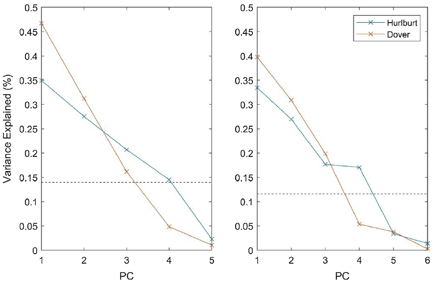
Regarding the bias-reduction benefits of PCR, rather than remove an IV suspected to be collinear or keep all IVs and ignore collinearity, PCR enables the retention of unique orthogonal signals without the loss of information (Abdi and Williams 2010). Dimensional reduction is addressed in this work through the use of Jolliffe’s Rule, which retains only the principal components (PCs) that describe at least a predetermined amount of variation in the model. Applying the ruleset also reduces the risk of overfitting. Here, Jolliffe’s Rule retains any PC that explains at least 70% of the mean variance explained by all PCs (Jolliffe 2002). Fig. 3 provides example scree plot results for Dover and Hurlburt, which illustrates how the number of retained PCs varies by location when using the thresholds from Jolliffe’s Rule.
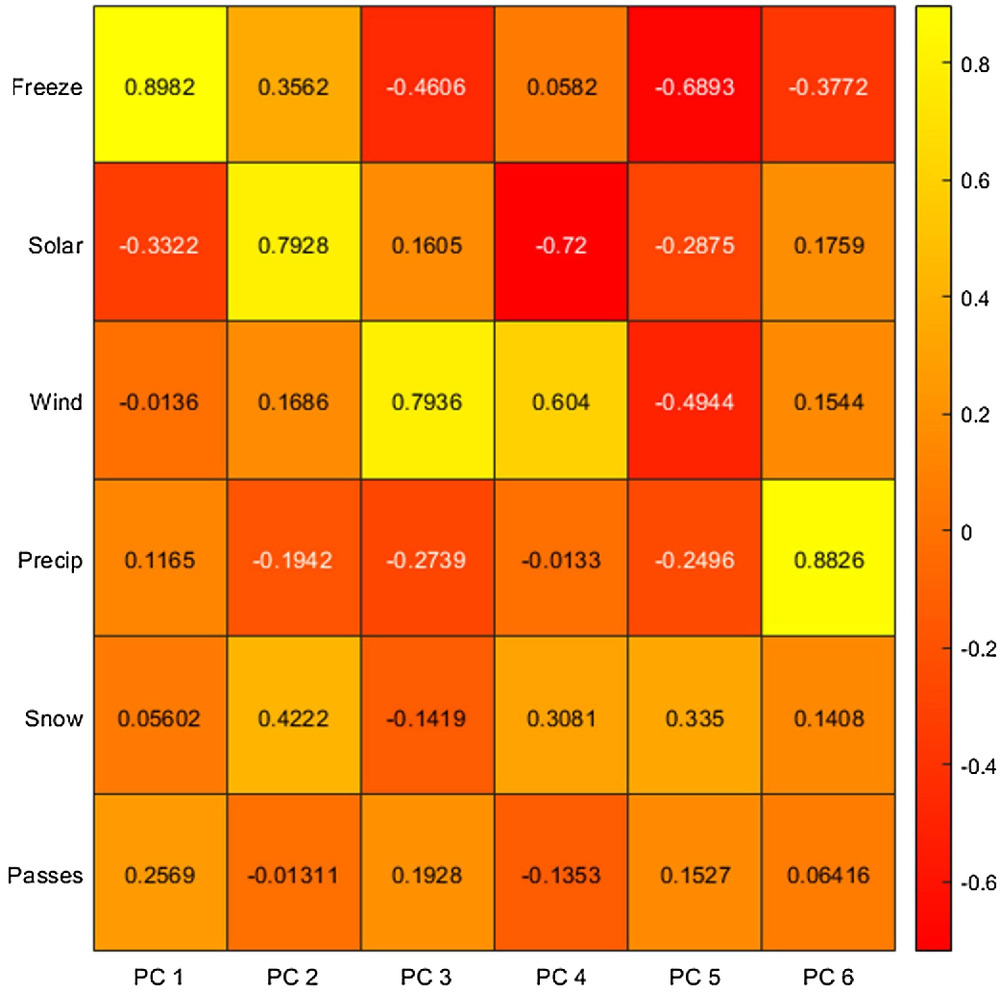
The PCs do not relate directly to any single IV. They must be exhaustively correlated with the IVs to determine the relationship between each PC and IV, as revealed through heat plots. An example of the correlation between PC and IV is as follows: if PC 1 is correlated with freeze-thaw at 0.9, with solar irradiance at , and with equivalent passes at 0.2, this means that the first mode of variability in the data set, PC 1, is primarily driven by freeze-thaw, but also has moderate and weak ties to solar irradiance and passes, respectively. While the remainder of IVs is present within PC 1, their correlations are negligible. This trusted process was repeated for every retained PC from every pavement family at every location, ultimately determining which IVs were significant and important for each unique pavement grouping.
Cross-validation is a bias-reduction technique. It was used to temporarily remove, or drop, the dependent variable observation for the time step, or time steps, surrounding the PCR prediction such that “perfect targets” are eliminated from consideration (Delorit et al. 2017). Since only the predicted condition value is dropped, the form used herein is referred to as drop-one cross-validation. Adding cross-validation to the multi-factor linear regression (MLR) process is expected to lower the Pearson’s correlation () because the model is not provided with the “target” datapoint. This tradeoff between model skill and bias is necessary to produce a fair set of predictions and test the framework’s validity.
The PCR approach was applied in two formulations: one that only included climate and another that included both climate and traffic passes. Using two different sets is meant to challenge existing approaches that use traffic only by revealing the individual impacts that climate and traffic passes have on pavement degradation for the period 2010–2019.
Results
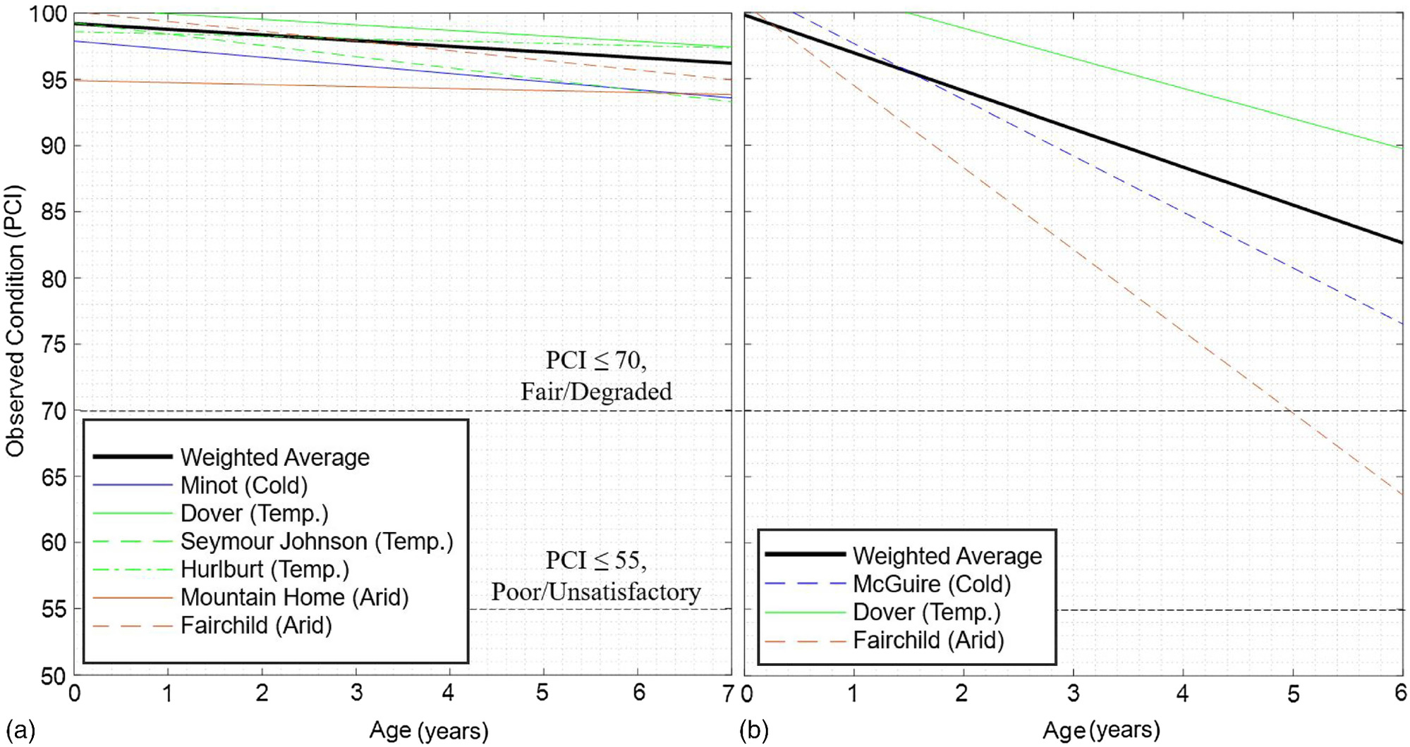
Examples of the linear approximations for Rig A’s continuous degradation functions with Flex A are shown in Fig. 4; these pavement types are the most important and heavily trafficked parts of the airfield. The lines for each location’s degradation rate are colored according to Köppen-Geiger zone, with green as the temperate zone, orange as arid, and blue as cold (Delorit et al. 2020). The solid black line is the weighted average of all locations within that family. Regardless of pavement makeup, a PCI of 70 is the threshold for when a pavement section is considered degraded and could receive some rehabilitative care; a condition of 55 represents failing sections that should be replaced (Greene et al. 2004). Dashed lines have been added at 70 and 55 to display the difference in the expected life cycle between rigid and flexible pavements, respectively. Over this timespan, flexible pavements are more variable and have a sharper degradation line. Fairchild Air Force Base (AFB) Flex A pavement sections fall within the degraded category within the first five years of the pavement life. Both Rig A and Flex A for Fairchild are below the weighted average of locations for these respective families. These findings suggest some abnormality with the conditions at Fairchild. For example, there are likely combinations of environmental factors, high traffic volumes, and aircraft conditions that are especially harmful to the airfield surfaces over short time scales, including extreme weather events (Oyediji et al. 2021; Lu et al. 2018). The coarse temporal resolution of traffic and PCI data obtained for this study prevented an assessment of combined, acute degradative events. Furthermore, the results could have been subject to statistical errors that arose from the short temporal scale of analysis and limited data points (only five pavement sections remained for Fairchild Flex A pavements that met the inclusion criteria and were constructed on or after 2010 due to aircraft pass data constraints).
Each continuous degradation function was used as the dependent variable in the cross-validated PCR model. and the root mean square error (RMSE) are used as deterministic model skill metrics. The statistical model outputs are post-processed to ensure a decreasing, monotonic relationship between time and degradation. Only predictions of degradation between time steps were accounted for. In cases where the model suggested pavement condition improvement between years, the condition value was held constant for that time step. This post-processing aligns with PAVER and better matches actual conditions.
The PCR model was first applied to all family-location pairs using only the five selected climatic IVs. Table 4 displays the and significance (-values) for all models when only considering climate. The significance was found before adjusting to the methodology in PAVER, so all families have the same value within each location since climatic conditions are experienced across the entire location equally. As expected, studying a limited period (10 years) produced -values that exceed accepted confidence levels. However, high confidence levels may not be necessary to enable pavement rehabilitation or replacement decisions. The “Limitations” section of this paper explores the tradeoff between model confidence and decision-making. A dash in Table 4 represents cases where pavement data was insufficient to issue statistically significant predictions. Given the reliability and longevity of pavements, the authors hypothesized that the effects of environmental influences would be minimal across 10 years; however, the models described between 30% and 84% of the variation in degradation, meaning that climate has a significant and powerful role in degradation even over short time spans. Too many data gaps existed to make conclusions about differences between model skill for families Rig C, Flex A, and Flex D. However, pavements within PCASE traffic designator A, the first 304.8 m (1,000 ft) of runways and all primary taxiways, are typically made from rigid pavements. Family Rig A has fewer limitations in data. Rig A will be further analyzed in the “Discussion” section because it has the most expected aircraft traffic, contains the most primary-designation sections, and may be considered the most important surface that supports aircraft operations. According to this analysis, traffic designator C, runway interiors, and secondary/tertiary taxiways are the most common flexible surfaces.
| Location | Significance (p-value) | Pearson’s coefficient of determination () | |||||
|---|---|---|---|---|---|---|---|
| Rig A | Rig B | Rig C | Flex A | Flex C | Flex D | ||
| Cold | |||||||
| McGuire | 0.50 | — | — | — | 0.40 | 0.39 | — |
| Minot | 0.78 | 0.36 | 0.32 | 0.35 | — | 0.40 | 0.30 |
| Temperate | |||||||
| Dover | 0.14 | 0.80 | 0.81 | — | 0.81 | 0.80 | — |
| Hurlburt | 0.16 | 0.51 | — | — | — | — | — |
| Moody | 0.11 | — | 0.58 | — | — | — | — |
| Seymour John | 0.42 | 0.38 | 0.34 | 0.40 | — | 0.45 | — |
| Arid | |||||||
| Fairchild | 0.12 | 0.72 | 0.71 | 0.71 | 0.72 | 0.73 | 0.71 |
| MtHome | 0.23 | 0.36 | — | — | — | — | — |
| Nellis | 0.013 | — | — | — | — | 0.84 | 0.65 |
Note: An em dash represents insufficient data for model application.
The same PCR model was run a second time, now inclusive of equivalent passes as an IV. Model skill was expected to increase, but based on previous research, the expectation was that skill would improve significantly when traffic was added. Almost every model application displayed increased skill, with an average change of . The values from the climate-only model set were divided by the results of the climate and passes model set to reveal the percentage of model skill attributed to climate. Table 5 displays this percentage and the difference in between the two model sets. Analysis of the model set comparison continues in the “Discussion” section.
| Location | Rig A | Rig B | Rig C | Flex A | Flex C | Flex D | ||||||
|---|---|---|---|---|---|---|---|---|---|---|---|---|
| Percentage (%) | Percentage (%) | Percentage (%) | Percentage (%) | Percentage (%) | Percentage (%) | |||||||
| Cold | ||||||||||||
| McGuire | — | — | — | — | — | — | 0.105 | 79 | 0.095 | 81 | — | — |
| Minot | 0.023 | 94 | 0.016 | 95 | 0.022 | 94 | — | — | 0.024 | 94 | 0.009 | 97 |
| Temperate | ||||||||||||
| Dover | 0.114 | 88 | 0.113 | 88 | — | — | 0.111 | 88 | 0.113 | 88 | — | — |
| Hurlburt | 0.011 | 98 | — | — | — | — | — | — | — | — | — | — |
| Moody | — | — | 0.089 | 87 | — | — | — | — | — | — | — | — |
| Seymour John | 0.068 | 85 | 0.039 | 90 | 0.083 | 83 | — | — | 0.126 | 78 | — | — |
| Arid | ||||||||||||
| Fairchild | 102 | 102 | 102 | 102 | 102 | 102 | ||||||
| MtHome | 0.014 | 96 | — | — | — | — | — | — | — | — | — | — |
| Nellis | — | — | — | — | — | — | — | — | 112 | 0.016 | 98 | |
Note: Percent values greater than 100 signify a case where adding traffic data reduced model performance.
Table 6 gives the error (RMSE) values produced by the model set that had both climate and pass data. RMSE is especially important when creating expectations that are used to schedule maintenance activities. Although the model used in this research is useful for understanding sources of degradation, this research is not concerned with having low error values since validation and further research are required to transform this model or merge its applications with PAVER to create a useful condition prediction tool. Still, low error values were found for most family-location pairs. The RMSE values for this final model set were less than 10 with few exceptions: Fairchild Flex A and most Flex C.
| Location | Root mean square error (PCI value) | |||||
|---|---|---|---|---|---|---|
| Rig A | Rig B | Rig C | Flex A | Flex C | Flex D | |
| Cold | ||||||
| McGuire | — | — | — | 9.37 | 6.80 | — |
| Minot | 1.86 | 0.45 | 1.46 | — | 12.92 | 2.72 |
| Temperate | ||||||
| Dover | 0.81 | 1.69 | 0.00 | 4.39 | 12.58 | — |
| Hurlburt | 0.41 | — | — | — | — | — |
| Moody | — | 1.04 | — | — | — | — |
| Seymour John | 2.09 | 1.49 | 5.18 | — | 15.90 | — |
| Arid | ||||||
| Fairchild | 1.79 | 8.74 | 0.61 | 14.99 | 3.64 | 4.55 |
| MtHome | 0.41 | — | — | — | — | — |
| Nellis | — | — | — | — | 3.76 | 0.93 |
| CI | ||||||
Fairchild AFB’s heat map is shown in Fig. 5 as an example of applying the established PC retention rules. Degradation variability is described in decreasing order of importance as freeze-thaw, solar, wind, and snow. The model retained freeze-thaw and solar irradiance within PC 1 because they are both above 0.4. Moreover, the highest correlation values for PC 2 and 3 were considered since 3 PCs were retained for this location. The equivalent passes IV is notable in the first PC but not more significant than any climate variables.
Discussion
The climate-passes model set reveals several interesting conclusions when compared to the climate-only model set. Dover had the largest increase in skill when adding passes, followed by Seymour Johnson AFB. Including pass data increased model skill by as much as 22% across all family-location pairs. This improvement suggests that aircraft passes describe a meaningful amount of degradation for this location. However, the observed model improvement was less than what the authors hypothesized, likely because climatic factors are more harmful to the pavements analyzed. Another explanation is that pavements are designed for the expected aircraft traffic at each location, and those design choices are performing well, thereby minimizing the model’s ability to detect trends in aircraft passes and pavement degradation. Climatic design considerations are not as advanced or tailored within pavement design criteria, which tangentially includes local data for freezing index, mean annual temperature, and frost season length (Van Steenburg, n.d.).
One notable conclusion from Table 4 is that the model values do not differ significantly between families within an installation because the climatic conditions are not variable at the installation scale. However, the RMSE indicates how well the model was able to replicate the continuous function for each family. As seen in Table 6, rigid families had significantly lower error values than Flex A and Flex C pavements, displaying the model’s ability to approximate the continuous function more accurately. This suggests that rigid pavements degrade more predictably than flexible when subjected to the same climatic influences, potentially due to better performance as shown by the low-sloped continuous functions.
Pavement family Rig A is the most important to mission support, and most locations provided enough data from this family to perform the model. Rig A’s RMSE values were less than 3. The scale of potential values for RMSE is the same as PCI (0–100). Across a 10-year window, the authors suggest that an error of less than 10 is acceptable, as it represents an average annual condition prediction error of one PCI point. Also, the model without aircraft passes ranged from 0.36 to 0.80 and only increased by 2%–15% when including passes. As expected, families with traffic type A are expected to receive the most aircraft traffic and experience the highest percent improvement in model skill. Still, the results from this research suggest that climate is a more meaningful contributor to pavement degradation than aircraft passes, and this study represents the first to quantify the unique contributions of each variable category.
Even though the percent of degradation variation is mostly described by climate, Fairchild AFB’s families surprisingly had slight decreases in , and Nellis AFB’s Flex C decreased by 0.09. Both locations are in the arid zones, but Fairchild AFB had the largest number of pavement sections (67), while Nellis AFB had the least (11). Fairchild AFB is further juxtaposed since that location also primarily flies large KC-135 aircraft, equivalent to a Boeing 717 with a gross takeoff weight of 146,510 kg. In comparison, Nellis AFB operates light F-16 fighter aircraft (17,010 kg), which are a full order of magnitude lighter than Fairchild AFB’s aircraft (UFC 2001b). Higher or lower values correspond with the model’s certainty in its ability to predict degradation effects, not with the strength of those effects. Nellis AFB’s lack of data hinders model performance. Acquiring additional pavement condition data would likely improve model skill, based on the model’s performance at bases with more data. Fairchild AFB, however, had enough data points to avoid these issues. Fig. 6 displays one possible explanation for the model’s inability to replicate degradation at Fairchild AFB. Fairchild AFB had strong degradative effects from many climatic sources with the second-highest coefficient of determination (). This suggests that the trends inherent in the climatic effects are strongly correlated with Fairchild AFB’s continuous degradation function, but the correlation between passes and degradation is weaker.
Using linear approximations for the continuous functions creates the potential for inflated model results; PCR implements MLR with PCs. By design, MLR will have the best results when applied to linear functions. The true nature of pavement condition depreciation is nonlinear, and as such, a linear model approach may lose skill as more data becomes available. In this case, nonlinear PCR methods should be explored. This limitation mainly applies when considering this model framework as a raw prediction tool. PAVER successfully creates accurate condition predictions, and the purpose of this model framework is to enhance existing capabilities by incorporating local condition variables and providing the capability to utilize future projections of climatic conditions to combat temporal uncertainty. The benefits provided through this model framework overcome any potential result inflation due to the linear approximations from the continuous functions.
Since the PCR model set retains the PCs that are the most meaningful in describing variation in pavement degradation, this process shows only the variables that have had the most significant impact on each location. Fig. 6 displays the important and significant climatic variables by location using correlation of the retained principal components with the independent variables. With further research, this knowledge could be compiled and recorded for use in current APMS as a module that creates more accurate predictions influenced by climate and use.
Aircraft passes were present in only one location, Fairchild AFB, where passes described 26% of the first PC. Even at this location, which had the largest presence of aircraft passes, this variable was still less significant than climate effects. Furthermore, the model dropped by 1%–2% for Fairchild when considering passes, despite almost all other locations gaining skill with pass inclusion. The detrimental effects of freeze-thaw were significant at every location and were the leading source of deterioration in five locations, mostly occurring in the cold and temperate zones. Freeze-thaw is a known degradative factor, and the model is further validated by its recognition of freeze-thaw’s impact. The presence of freeze-thaw as a significant variable in the arid zone and southwestern US locations can be attributed to a few factors: pavement design in arid locations may not use additives or construction techniques to combat the effects of freeze-thaw, and fewer freeze-thaw days means that annual differences of freeze-thaw recurrence would make up a larger percentage of change and be more heavily accounted for by the models.
Solar irradiance was significant at every location, and to the author’s knowledge, this is the first study to directly quantify its effect on airfield pavements, other than tangentially through temperature gradients. It was the leading degradation source in three locations, and as expected, it had the strongest presence in the arid zone. The pervasive appearance of solar irradiance implies a strong effect on pavement degradation. Irradiance levels remain relatively constant between years and by location, which could confound the model results. The regression model gives consistent zero-sloped trends more weight due to similarities with the linear, low-sloped continuous functions. Regardless, solar irradiance is rarely accounted for in pavement design or pavement life cycle rehabilitation; therefore, novel discovery can motivate research into the sun’s effect on pavement surfaces.
Snowfall depth was only significant at two locations, Fairchild AFB and McGuire AFB. Many locations that receive snow have extensive snow-removal programs to ensure steady aircraft operations. Snow-removing equipment interacts with pavements. Using snowfall as a variable was intended to capture snow-removal operation’s role in explaining degradation. By removing snowfall, any potential detrimental effects of snowfall may be mitigated and therefore absent in Minot and Dover, which received large amounts of snow throughout the observed period.
Limitations
Several assumptions were made to address identified limitations and uncertainty. The first main limitation was the amount of aircraft pass data. Since ATAR records have only been compiled since 2010, the data’s temporal extent is a limiting factor, and the results should be viewed as meaningful, but only for the short period of data available. An initial review of PAVER data revealed the possibility to include 1,995 pavement sections from 14 locations, with a longer temporal record (1985–2019), but only 266 pavement sections remained that were constructed after 2010 between 9 remaining locations; 5 locations from the original data had so few data points with this constrained timeframe that they were removed from the analysis. The number of data points per location varied from 11 to 67, creating many gaps where pavement families could not be analyzed, and the significance of the models ranged from 51% to 99% (). However, high confidence intervals (CI) may not be necessary for pavement deterioration analysis. The data’s fidelity and consistency allow for lower CI that still discovers the importance of model contributors, the largest sources of deterioration among the included variables. Pavement design engineers and asset managers understand that there are many degradation sources, so identifying specific threats, as was accomplished with this research, is beneficial regardless of confidence level.
Another source of uncertainty surrounded the creation of the equivalent passes variable. The internal, empirically based calculations in PCASE were trusted to determine equivalent passes through a module that is not the primary function of this design software. Rounding errors may have also been an issue since the number of acceptable passes used to determine equivalent passes was 50,000 from a C-17, resulting in very high pass values for smaller fighter aircraft. Several conditions were assumed to be static between airfields since the data was unavailable, such as subgrade condition strength and failure criteria. PCASE’s standard values were used, although the authors recognize that differences in construction standards and materials will affect these variables. Aircraft operation uncertainty also influenced the creation of the equivalent passes variable, which assumed a single, leading aircraft as the cause of deterioration at an installation.
Real-world aircraft operations are unpredictable. The heaviest permanently stationed aircraft is likely the leading contributor to pavement damage. However, many other aircraft of varying weights and wheel configurations regularly operate stochastically between airfields depending on mission requirements. The aircraft pass data represents all passes without distinguishing aircraft, introducing even more uncertainty. Several assumptions were made such that design criteria match the experienced conditions, but this cannot always be accurate, such as with aircraft wander width. Critical overloading of pavement is another source of uncertainty that significantly increases pavement damage. This overloading can be caused by aircraft that are heavier than the design conditions or aircraft mishaps (e.g., no landing gear, fire on the airfield, or aircraft crash).
The final main limitation for this research was the lack of pavement design data. The information provided in the PAVER summary reports did not give specifics on the range of available choices for PCC or hot mix asphalt (HMA) mixture designs, potential additives, or the quality or type of subgrade and subbase materials. These design factors are typically tailored to their location and attempt to minimize the effects of environmental factors. Without this information, the model is effectively applied using the families of like-type pavements with the assumption that all pavements have a consistent application of localized design and that all concrete construction was performed to the specifications and in good faith by the contractors and design agents at each installation. Further research can be performed that identifies the specific, localized mix design qualities and performs iterations of this model application to determine those effects.
Conclusions
This research constructed an adaptable, climate- and traffic-informed statistical pavement deterioration prediction framework and tested its transportability on a data set of 9 USAF airfields. Three steps are performed to accomplish the research objectives that amplify capability from PAVER: (1) pavement families with similar qualities of type (material), rank (priority), and use (location) were grouped using standardized criteria; (2) individualized, linear degradation functions were generated as a target for modeling on each of the selected family-location pairs; and (3) a bias-reduced, principal component regression model was applied to each of these family-location pairs across a temporal scale of 10 years, from 2010 to 2019, such that correlation of the PCs to the IVs revealed the significance and strength of variable impact. The models described between 36% and 92% of the variation in degradation, meaning that the selected climate variables and aircraft passes have a significant and influential role in degradation of both rigid and flexible pavements even over short time frames.
This novel system framework is flexible and can be applied to any combination of location and pavement type using variables of interest that have matching temporal resolutions and data availabilities. This research’s key finding is that APMSs and pavement design engineers must account for local climate in the management of pavements to promote surface longevity and more accurately plan preventive and corrective maintenance and repair interventions. As climate changes, the variables that currently degrade pavements may be amplified, intensifying the effects on pavement deterioration, or may change altogether; this framework can adapt by using forecasted condition time series. Although DoD data sets were analyzed herein, both commercial and private airfields could benefit from developing advanced APMS software that would enable better, data-driven, and effective decision-making.
A comparison of model configurations revealed that climate describes a far larger percentage of variation than aircraft passes, with passes increasing model skill by only 14% on average. The small increased benefit of including passes suggests that climatic conditions have a larger degradative effect or that pavements are successfully designed according to the expected aircraft travel and not climate. Freeze-thaw and solar irradiance are commonly significant degradative sources and were prevalent throughout the contiguous United States. Although aircraft passes were shown to be more detrimental to flexible pavements than rigid, aircraft passes were not among the leading influences at any installation considered in this analysis.
Data Availability Statement
Some or all data, models, or code generated or used during the study are proprietary or confidential in nature and may only be provided with restrictions (e.g., anonymized data). (AccuWeather proprietary database is available for purchase from vendor; AFFSA annual aircraft passes found in the ATAR available with appropriate security clearances upon request from the unit.)
References
Abdi, H., and L. J. Williams. 2010. “Principal component analysis.” WIREs Comput. Stat. 2 (4): 433–459. https://doi.org/10.1002/wics.101.
Abed, A., N. Thom, and L. Neves. 2019. “Probabilistic prediction of asphalt pavement performance.” Supplement, Road Mater. Pavement Des. 20 (S1): S247–S264. https://doi.org/10.1080/14680629.2019.1593229.
Adolf, M. 2010. PCASE 2.09 user manual. Washington, DC: USACE, Transportation Systems Center and Engineering Research and Development Center.
AFI (Air Force Instruction). 2019. Compliance with this publication is mandatory. AFI 32-1041. Washington, DC: Civil Engineering Pavement Evaluation Program, Dept. of the Air Force.
Allen, J. P., and B. C. Albert. 2014. Sustainable transportation: Strategy for security, prosperity, and peace. Carlisle, PA: US Army War College.
Ameri, M., A. Mansourian, M. Heidary Khavas, M. R. M. Aliha, and M. R. Ayatollahi. 2011. “Cracked asphalt pavement under traffic loading—A 3D finite element analysis.” Eng. Fract. Mech. 78 (8): 1817–1826. https://doi.org/10.1016/j.engfracmech.2010.12.013.
Ankit, G., P. Kumar, and R. Rastogi. 2011. “Effect of environmental factors on flexible pavement performance modeling.” In Proc., 8th Int. Conf. on Managing Pavement Assets (ICMPA8). Santiago, Chile: Pontificia Universidad Catolica de Chile College of Engineering.
ASTM. 2012. Standard test method for airport pavement condition index surveys. ASTM D5340-12. West Conshohocken, PA: ASTM.
Beck, H. E., N. E. Zimmermann, T. R. McVicar, N. Vergopolan, A. Berg, and E. F. Wood. 2018. “Present and future Köppen-Geiger climate classification maps at 1-km resolution.” Sci. Data 5 (1): 180214. https://doi.org/10.1038/sdata.2018.214.
Bennett, M. 2019. “Factors affecting airfield pavement performance in the United States Air Force enterprise wide.” Master of Science, Dept. of Civil Engineering, Pennsylvania State Univ.
Brown, S. 2021. “Investigating manufacturer selection decisions for built infrastructure assets using a technical performance metric.” Master of Science in Engineering Management, Air Force Institute of Technology, Graduate School of Engineering and Management.
Chih-Yuan, C., and P. L. Durango-Cohen. 2008. “Empirical comparison of statistical pavement performance models.” J. Infrastruct. Syst. 14 (2): 138–149. https://doi.org/10.1061/(ASCE)1076-0342(2008)14:2(138).
Chinowsky, P. S., J. C. Price, and J. E. Neumann. 2013. “Assessment of climate change adaptation costs for the US road network.” Global Environ. Change 23 (4): 764–773. https://doi.org/10.1016/j.gloenvcha.2013.03.004.
CSU (Colorado State University). 2019. “About PAVER.” Accessed March 12, 2020. http://www.paver.colostate.edu/.
Delorit, J., E. C. Gonzalez Ortuya, and P. Block. 2017. “Evaluation of model-based seasonal streamflow and water allocation forecasts for the Elqui Valley, Chile.” Hydrol. Earth Syst. Sci. 21 (9): 4711–4725. https://doi.org/10.5194/hess-21-4711-2017.
Delorit, J. D., S. J. Schuldt, and C. M. Chini. 2020. “Evaluating an adaptive management strategy for organizational energy use under climate uncertainty.” Energy Policy 142 (Jul): 111547. https://doi.org/10.1016/j.enpol.2020.111547.
FAA (Federal Aviation Administration). 2014. Airport pavement management program (PMP), advisory circular (AC). Washington, DC: US DOT, FAA.
Fortney, E. 2021. “Improving airfield pavement degradation prediction skill with local climate and traffic.” Master’s thesis, Air Force Institute of Technology, Graduate School of Engineering and Management.
Frangopol, D. M., J. S. Kong, and E. S. Gharaibeh. 2001. “Reliability-based life-cycle management of highway bridges.” J. Comput. Civ. Eng. 15 (1): 27–34. https://doi.org/10.1061/(ASCE)0887-3801(2001)15:1(27).
Gendreau, M., and P. Soriano. 1998. “Airport pavement management systems: An appraisal of existing methodologies.” Transp. Res. Part A Policy Pract. 32 (3): 197–214. https://doi.org/10.1016/S0965-8564(97)00008-6.
Greene, J., M. Y. Shahin, and D. R. Alexander. 2004. “Airfield pavement condition assessment.” Transp. Res. Rec. 1889 (1): 63–70. https://doi.org/10.3141/1889-08.
Haas, R. 2001. “Reinventing the (pavement management) wheel.” In Proc., 5th Annual Conf. on Managing Pavements. Seattle: Univ. of Washington.
Harvey, J. T., J. Meijer, H. Ozer, I. L. Al-Quadi, A. Saboori, and A. Kendall. 2016. Pavement life cycle assessment framework, 244. Washington, DC: US DOT, Federal Highway Administration.
Heymsfield, E., and J. S. Tingle. 2019. “State of the practice in pavement structural design/analysis codes relevant to airfield pavement design.” Eng. Fail. Anal. 105 (Nov): 12–24. https://doi.org/10.1016/j.engfailanal.2019.06.029.
Ismail, N., A. Ismail, and R. Atiq. 2009. “An overview of expert systems in pavement management.” Eur. J. Sci. Res. 30 (1): 99–111.
Jolliffe, I. T. 2002. “Choosing a subset of principal components or variables.” In Principal component analysis, 111–149. New York: Springer.
Kaewunruen, S., L. Wu, K. Goto, and Y. M. Najih. 2018. “Vulnerability of structural concrete to extreme climate variances.” Climate 6 (2): 40. https://doi.org/10.3390/cli6020040.
Kjellstrom, T., C. Freyberg, B. Lemke, M. Otto, and D. Briggs. 2018. “Estimating population heat exposure and impacts on working people in conjunction with climate change.” Int. J. Biometeorol. 62 (3): 291–306. https://doi.org/10.1007/s00484-017-1407-0.
Li, R., C. W. Schwartz, and B. Forman. 2013. “Sensitivity of predicted pavement performance to climate characteristics.” In Proc., Airfield and Highway Pavement 2013: Sustainable and Efficient Pavements, 760–771. Reston, VA: ASCE.
Lu, D., S. L. Tighe, and W.-C. Xie. 2018. “Pavement risk assessment for future extreme precipitation events under climate change.” Transp. Res. Rec. 2672 (40): 122–131. https://doi.org/10.1177/0361198118781657.
Meihaus, J. C. 2013. “Understanding the effects of climate on airfield pavement deterioration rates.” Master's thesis, Air Force Institute of Technology, Graduate School of Engineering and Management.
Mulry, B., M. Jordan, and D. O’Brien. 2015. “Automated pavement condition assessment using laser crack measurement system (LCMS) on airfield pavements in Ireland.” In Proc., 9th Int. Conf. on Managing Pavement Assets. Blacksburg, VA: Virginia Tech Transportation Institute.
Oyediji, R., D. Lu, and S. L. Tighe. 2021. “Impact of flooding and inundation on concrete pavement performance.” Int. J. Pavement Eng. 22 (11): 1363–1375. https://doi.org/10.1080/10298436.2019.1685671.
Parsons, T. A., and B. A. Pullen. 2016. “Relationship between climate type and observed pavement distresses.” In Proc., Int. Conf. on Transportation and Development 2016, 88–102. Reston, VA: ASCE.
Parsons, T. A., and B. A. Pullen. 2017. “Characterization of pavement condition index deterioration curve shape for USAF airfield pavements.” In Proc., Airfield and Highway Pavements 2017, 230–240. Reston, VA: ASCE.
Qiao, Y., A. R. Dawson, T. Parry, G. Flintsch, and W. Wang. 2020. “Flexible pavements and climate change: A comprehensive review and implications.” Sustainability 12 (3): 1057. https://doi.org/10.3390/su12031057.
Sahagun, L. K., M. Karakouzian, A. Paz, and H. de la Fuente-Mella. 2017. “An investigation of geography and climate induced distresses patterns on airfield pavements at US Air Force installations.” Math. Probl. Eng. 2017. https://doi.org/10.1155/2017/8721940.
Sawant, V. 2009. “Dynamic analysis of rigid pavement with vehicle-pavement interaction.” Int. J. Pavement Eng. 10 (1): 63–72. https://doi.org/10.1080/10298430802342716.
Seiler, W. J., M. I. Darter, and J. H. Garrett. 1991. “An airfield pavement consultant system (AIRPACS) for rehabilitation of concrete pavements.” In Proc., Aircraft/Pavement Interaction: An Integrated System, 332–353. New York: ASCE.
Shafabakhsh, G. A., and E. Kashi. 2015. “Effect of aircraft wheel load and configuration on runway damages.” Period. Polytech., Civ. Eng. 59 (1): 85–94. https://doi.org/10.3311/PPci.2103.
Shahin, M. Y. 1994. “Analyzing consequences of pavement maintenance and rehabilitation budget scenarios.” Transp. Res. Rec. 1455: 166–171.
Shahin, M. Y. 2005. Pavement management for airports, roads, and parking lots. New York: Springer.
Shahin, M. Y., M. M. Nunez, M. R. Broten, S. H. Carpenter, and A. Sameh. 1987. “New techniques for modeling pavement deterioration.” Transp. Res. Rec. 1123: 40–46.
Shahin, M. Y., and F. M. Rozanski. 1978. “Development of a computerized system for pavement maintenance management.” Transp. Res. Rec. 674: 3–11.
Sidess, A., A. Ravina, and E. Oged. 2021. “A model for predicting the deterioration of the pavement condition index.” Int. J. Pavement Eng. 22 (13): 1625–1636. https://doi.org/10.1080/10298436.2020.1714044.
Taylor, M. A. P., and M. L. Philp. 2015. “Investigating the impact of maintenance regimes on the design life of road pavements in a changing climate and the implications for transport policy.” Transp. Policy 41 (Jul): 117–135. https://doi.org/10.1016/j.tranpol.2015.01.005.
UFC (Unified Facilities Criteria). 2001a. Airfield pavement design. UFC 3-260-03. Washington, DC: US Dept. of Defense, UFC.
UFC (Unified Facilities Criteria). 2001b. Pavement design for airfields. UFC 3-260-02. Washington, DC: US Dept. of Defense, UFC.
Van Steenburg, G. n.d. “PCASE on-line design workshop.” Accessed March 26, 2021. https://transportation.erdc.dren.mil/tsmcx/training.aspx.
Van Vuuren, D. P., J. Edmonds, and M. Kainuma. 2011. “The representative concentration pathways: An overview.” Clim. Change 109 (5): 5–31. https://doi.org/10.1007/s10584-011-0148-z.
Wang, H., and I. L. Al-Qadi. 2011. “Impact of non-uniform aircraft tire pressure on airfield pavement responses.” In Proc., Transportation and Development Institute Congress 2011: Integrated Transportation and Development for a Better Tomorrow, 844–853. Reston, VA: ASCE.
White, T. D., S. M. Zaghloul, G. L. Anderton, and D. M. Smith. 1997. “Pavement analysis for moving aircraft load.” J. Transp. Eng. 123 (6): 436–446. https://doi.org/10.1061/(ASCE)0733-947X(1997)123:6(436).
Information & Authors
Information
Published In

Journal of Transportation Engineering, Part B: Pavements
Volume 148 • Issue 2 • June 2022
Copyright
This work is made available under the terms of the Creative Commons Attribution 4.0 International license, https://creativecommons.org/licenses/by/4.0/.
History
Received: May 5, 2021
Accepted: Dec 20, 2021
Published online: Mar 11, 2022
Published in print: Jun 1, 2022
Discussion open until: Aug 11, 2022
Authors
Metrics & Citations
Metrics
Citations
Download citation
If you have the appropriate software installed, you can download article citation data to the citation manager of your choice. Simply select your manager software from the list below and click Download.
Cited by
- Hakan Turan, Muhammet Enis Bulak, Sustainable Performance Evaluation for European Airports With Principal Component Approach, Considerations on Education for Economic, Social, and Environmental Sustainability, 10.4018/978-1-6684-8356-5.ch011, (222-241), (2023).