Hydrodynamic Simulations for Trash Loading in Southern California’s Dense Urbanized Watersheds
Publication: Journal of Environmental Engineering
Volume 150, Issue 8
Abstract
Waterways and water bodies worldwide are impacted by anthropogenic litter (hereafter “litter” or “trash”), generated from nonpoint sources. This study analyzes litter loads across various land uses within two Los Angeles County watersheds: the Ballona Creek and the Los Angeles River. Our objective is to present a methodology to develop buildup and washoff parameters for densely populated urban areas, such as the coastal metropolitan area of Los Angeles, California. An assessment is also made to test how these model parameters perform when applied to another urbanized watershed with similar rainfall and climate patterns (i.e., the San Diego River Watershed in California). Using extensive litter collection data from small drainages (approximately 572 locations, each draining 0.05–8.5 ha), we estimate buildup and washoff model parameters. These parameters are used to simulate the buildup of litter and subsequent washoff (load) of litter in our selected watersheds. Simulated results are validated against observed data from different years in all three watersheds. To date, no study has used litter washoff data to develop these parameters for stormwater models and applied them on a regional scale. We compared linear and nonlinear power functions of litter buildup during interstorm periods. Although there were limited data to develop washoff parameters, an exponential washoff function was used and calibrated to the observed washoff. Generally, storm events with the greatest antecedent dry days had the largest litter loading. Buildup rates varied among land uses, and key calibration parameters included the maximum buildup, buildup rate constant, washoff exponent, and washoff coefficient. A parameter sensitivity analysis was conducted to reveal the washoff exponent as the most sensitive parameter. Annual litter loading estimates were for the Ballona Creek and for the Los Angeles River. Litter loading estimates for Ballona Creek were validated and calibrated to align with observed data from the Ballona Creek Trash Interceptor, resulting in an annual washoff load of . The estimated annual litter loading for the Lower San Diego River was falling between the mean () and the maximum () observed values. When applying model parameters from one watershed to another, models require extensive calibration and validation data, as extrapolating data between watersheds can introduce errors.
Practical Applications
This research can inform stormwater modelers about the process for developing parameters to estimate water quality in numerical modeling software. We demonstrate how data from field sampling can be directly used to develop model parameters. Results show that with proper validation data, stormwater models can accurately simulate annual litter loads in modeled watersheds. Future studies can test model parameters in other urbanized watersheds to validate the potential for standardized buildup values. Field studies can be done in conjunction with the results from this survey to investigate and further validate litter loads mobilized by stormwater. This study highlights the need for long-term monitoring to improve and update models in the future. Although there is a risk of inaccurate results when extrapolating model parameters from one watershed to another, this research indicates the potential for developing buildup and washoff parameters that can be used as a starting point for parameter selection across urban watersheds.
Introduction
Aquatic environments are heavily impacted by litter from nonpoint sources (Alam et al. 2018; Hossain et al. 2012; Kim and Kang 2004; Liang et al. 2019; Wicke et al. 2012). Trash on beaches and in waterways is aesthetically unappealing and poses potential dangers to marine organisms, causing economic impacts and potential long-term harm to the marine environment (Gold et al. 2015; Moore et al. 2016) and possibly human health (Prata et al. 2020). Litter or trash can be defined as any improperly discarded waste material, including, but not limited to, convenience food, beverage, product packages, or containers constructed of steel, aluminum, glass, paper, plastic, and other natural and synthetic materials (California Regional Water Quality Control Board Los Angeles Region 2001).
Estimation and control of litter loads is being increasingly incorporated into policy and management, including in California. Under Clean Water Act section 303(d), states are required to establish total maximum daily loads (TMDLs), the maximum amount of a pollutant that a waterbody can receive and still meet water quality standards, for any body of water that is impaired (Kim 2002). The California State Water Resources Control Board established TMDLs for trash or litter in some of Southern California’s urbanized watersheds, while allocating pollutant loadings to point and nonpoint sources (California Regional Water Quality Control Board Los Angeles Region 2001). In 2001, the California Regional Water Quality Control Board (CRWQCB) for the Los Angeles (LA) Region developed TMDLs for litter in the Ballona Creek Watershed. The CRWQCB for the LA Region (2001) identified three transport mechanisms for litter: rainstorms, wind, and direct disposal. The amount of trash that entered the stormwater system depended on the energy available to remobilize and transport litter, rather than on the amount of available litter; therefore, the main limitation for litter loads appears to be stormwater discharge rates and velocities (California Regional Water Quality Control Board Los Angeles Region 2001).
The County of LA Department of Public Works (LADPW) conducted a trash baseline study in the Los Angeles River Watershed and Ballona Creek Watershed from 2002 to 2004 (County of Los Angeles Department of Public Works Watershed Management Division 2004). The Los Angeles County Baseline Study (LACBS) installed about 500 catch basin inserts with contributing watersheds containing the following land uses: high-density single family residential (HDSFR), low-density single family residential (LDSFR), commercial, industrial, and open space/parks. Each catch basin insert received runoff from a single land use. Our research uses their findings to develop parameters for estimating litter loading during storm events. The goal is to apply these parameters to the LA County Watersheds and the Lower San Diego River Watershed (LSDRW) in San Diego, CA.
Litter loading for a specific storm event is determined by a combination of land use, event magnitude, and number of antecedent dry days. Researchers have quantified the loading rates of anthropogenic and natural litter transported by stormwater into the drainage system. Field investigations are designed with capture devices placed at the outlet of subcatchments to collect litter after rain events (Alam et al. 2018; BASMAA 2014; Michael Baker International 2018; Weideman et al. 2020; Winston et al. 2023). The collected gross solids (urban stormwater pollutants composed of organic material, litter, and large particulate matter) are then sorted to determine the loading rates of anthropogenic litter. One limitation in these studies is the collection frequency from the capture devices, given that a single sample could represent debris mobilized during dry weather events or one (or several) precipitation events (Winston et al. 2023). When analyzing urbanized watersheds, different land use categories have varying rates of litter deposition (Weideman et al. 2020). Gross pollutant loads are affected by seasonal conditions, where they were highest during the winter months due to mobilization by storms and rainfall. In the dry months, it is suspected that wind is the greatest factor for gross pollutant loading (Alam et al. 2017). Winter storms are capable of mobilizing litter with just a few millimeters of rainfall (Alam et al. 2018; Kim et al. 2004; Weideman et al. 2020; Winston et al. 2023). The above-mentioned studies confirmed that stormwater is capable of mobilizing litter from urban surfaces into catchment drains. Results from these studies, in terms of daily and annual loading rates, are presented in the results section of this paper.
Another limitation of capturing and measuring gross solids at stormwater outlets can be the limited range of field studies. Visual assessments of trash with vehicle mounted cameras or other devices is a qualitative way to identify litter available for transport into the storm drain system with rapid investigation (BASMAA 2014; Conley et al. 2022; Michael Baker International 2018). Aerial surveys with drone imagery can also advance the scale of litter assessments (Martin et al. 2021). Both aerial surveys with drone imagery and photos taken by cameras mounted on vehicles can utilize machine learning to identify areas of trash accumulation (Conley et al. 2022; Martin et al. 2021). Once generation rates have been developed with the aforementioned techniques, Geographical Information System (GIS) mapping can be used to delineate land use boundaries and apply litter generation rates to the total catchment area for a given land use (Martinez and Griffiths 2023). The present research uses the functionality of a popular numerical stormwater simulation software, PCSWMM, and localized field data to provide another approach for estimating litter in urban areas.
Buildup/Washoff Models
Buildup and washoff of litter can be clearly seen with visual assessment (Conley et al. 2022) and collection from catch basin inserts (Alam et al. 2017; BASMAA 2014; Weideman et al. 2020; Winston et al. 2023). The challenge is to use the data generated from field investigations to make generalizable parameters that can be used across multiple watersheds in urbanized regions. Difficulties arise when modeling washoff of litter from its place of deposition, which is a complicated function of several factors including antecedent dry period, density, and rainfall characteristics (Chaudhary et al. 2021).
Sartor et al. (1974) were the earliest researchers to implement the two main equations to simulate pollutant transport by stormwater (i.e., buildup, and washoff). Water quality models have since transitioned from mainly statistical, relying on linear regressions between different parameters and pollutant concentrations or loads, to deterministic, linking pollutant concentrations to conceptual processes and physical descriptions. The benefit of this transition is, now, distributed models distinguish land use types in subwatersheds or in grid cells, avoiding a lumped model where land use is assumed uniform. The buildup and washoff parameters can range widely so a priori estimation can be difficult. Additionally, data are often limited for model calibration, and water quality functions may not apply when shifting from small scales to the entire catchment (Bonhomme and Petrucci 2017).
Within the distributed model framework, pollutant loading models assume that constituents build up on the land surface in dry periods between storms. Concentrations of gross pollutants (litter and vegetation) increase with increasing numbers of antecedent dry days (Kim et al. 2004) and buildup rates typically decrease over time due to wind or vehicle-induced redistribution, where the total amount of material eventually reaches a maximum buildup per unit area (Alley and Smith 1981; Wicke et al. 2012).
To use the equations first presented by Sartor et al. (1974), researchers use existing literature to select appropriate values for modeling pollutant loading (Tu and Smith 2018; Tuomela et al. 2019) and calibrate values for common pollutants and indicators such as biological oxygen demand, chemical oxygen demand, total coliforms, total nitrogen, total phosphorus, and total suspended solids (TSS) (Alam et al. 2018; Rossman and Huber 2016; Tetra Tech 2010; Tu and Smith 2018; Wicke et al. 2012). Alternatively, researchers can conduct site experiments to collect data to develop buildup and washoff parameters (Hossain et al. 2010). For example, runoff and TSS concentrations can be collected from field data from road and roof surfaces, then best-fit buildup and washoff curves can determine relationships between pollutant buildup and washoff with respect to antecedent dry days and rainfall-runoff (Hossain et al. 2010). Our research uses a similar approach calibrating the same parameters utilized by Hossain et al. (2010) in the Gold Coast, Australia (i.e., maximum buildup possible, buildup rate constant, washoff coefficient, and washoff exponent).
There is a gap in understanding and lack of standardization for the buildup and washoff parameters relating to anthropogenic litter. Most buildup parameters for other constituents (maximum buildup and the buildup rate constant) are concentrated in a narrow range, which may indicate that pollutant buildup is controlled by factors that are spatially uniform (Tu and Smith 2018). On the contrary, washoff was found to be controlled by local factors such as topography, slope, infiltration capacity, and antecedent moisture, which influence runoff rate (Tu and Smith 2018). The studies with information on the buildup rates by land uses and estimates of annual litter loading (Armitage 2007; Armitage and Rooseboom 2000; BASMAA 2014; Hadiuzzaman et al. 2022; Martinez and Griffiths 2023; Weideman et al. 2020; Winston et al. 2023) have not been directly applied and calibrated in stormwater modeling software.
Sensitivity Analysis and Calibration
A sensitivity analysis (SA) is conducted to determine how the sensitivity of certain parameters can impact the model output (Lehtinen 2014). In the case of a buildup and washoff model, a SA can determine which parameters can influence litter loading the most. Both local and global methods exist for SA of hydrological models, such as screening methods, regression-based methods, and variance-based methods (Hong et al. 2019). Local SA methods or one-at-a-time methods determine the changes in model outputs from incremental changes in a single input parameter (Sun et al. 2012). A local SA is inefficient when more than one parameter controls the model output, because each parameter can directly affect the model output and indirectly effect other parameters. Local SA also fails to analyze the effect of large parameter changes (Sun et al. 2012). The Morris method ranks different parameters according to their sensitivities, while avoiding high computational cost of regression-based and variance-based methods. The Morris method averages local sensitivity measurements taken at different points of evenly spaced increments over a portion of the parameter range. This method is therefore a global method, as it explores a region of the parameter space (Chen et al. 2019; Vanrolleghem et al. 2015). The modified Morris method has been widely accepted as the standard for screening exercises (Hao et al. 2021; Li et al. 2016, 2020; Ma et al. 2021; Mohammed et al. 2022; Peng et al. 2020; Zhong et al. 2023).
Calibration of storm water management models (SWMM) washoff models can be difficult due to the variability among storm events, and reproducing the time variation of washoff concentration may be too difficult of a task given the simplified representation of the washoff process in SWMM. This simplified approach only considers how a given runoff rate can washoff available pollutants, ignoring aspects of the land surface and differences in pollutant size or structure. It is more realistic to calibrate against the total mass of washoff produced over a number of storm events rather than focus on individual storm events (Rossman and Huber 2016). Tetra Tech (2010) utilized this approach and adjusted model parameters until a target annual load was simulated within an acceptable percent difference from observed data.
Main Objectives
This paper addresses the research questions:
1.
What is the process to develop buildup and washoff parameters to model litter loading in an urban area?
2.
How are antecedent days and storm magnitude incorporated into buildup and washoff parameter development?
Our objective is to present a methodology to develop buildup and washoff parameters for densely populated urban areas. Using localized litter collection data at a small catchment scale, we develop and test the performance of these parameters for two watersheds within LA County, a coastal metropolitan area that meets the above criteria. An assessment is also made to test how these model parameters perform when applied to another urbanized watershed with similar rainfall and climate patterns, such as the San Diego River Watershed.
Data and Methods
The following section introduces the study areas, the incorporated datasets used for buildup and washoff parameter development, and the governing equations used for parameter development. Following the parameter development section, information on hydrologic verification and validation of the developed parameters is presented. Last, a brief section presents the street sweeping functionality within PCSWMM.
Study Areas
Three watersheds were analyzed for the purpose of this study: the Los Angeles River Watershed (LARW), Ballona Creek Watershed (BCW), and Lower San Diego River Watershed (LSDRW) (Fig. 1). These watersheds were selected due to data availability, similarity in rainfall patterns (short and episodic in the fall and winter months), and common levels of urbanization. The episodic nature of rainfall in these areas, combined with the increase in imperviousness across urban surfaces, leads to a flushing of pollutants into receiving waters (Holt et al. 2017). Mean annual rainfalls for the BCW, LARW, and LSDRW are 411 mm, 528 mm, and 498 mm, respectively. The LARW and BCW are adjacent. LARW covers approximately 216,000 ha and its main stem is approximately 82-km long from the Santa Monica Mountains to the Pacific Ocean. The river channel is 94% concrete banks and about 75% hard concrete bottom (Boroon and Coo 2015). The LARW is characterized by steep mountainous headwaters and low-lying flat sections in the San Fernando Valley. The LARW has a population of approximately 9 million people, with 43 cities plus unincorporated communities. The land uses are 37% residential, 8% commercial, 11% industrial, and 44% open space (Los Angeles County Public Works 2023b).

The BCW covers approximately 33,600 ha and is one of the most heavily developed watersheds in Southern California, with 61% impervious land cover (Gold et al. 2015). Due to channelization and imported water use, Ballona Creek has shifted from naturally ephemeral to perennial (Gold et al. 2015). The BCW also extends into the Santa Monica Mountains, and spans major cities: Beverly Hills, West Hollywood, unincorporated areas of LA County, parts of Culver City, and Inglewood. The BCW drains into Santa Monica Bay (Fig. 1). The BCW has approximately 1.5 million people and the following land uses: 64% residential, 4% industrial, 24% open space/other, and 8% commercial (Los Angeles County Public Works 2023a).
The entire San Diego River Watershed drains 111,628 ha to its discharge point at the Pacific Ocean. Two large dams hydrologically separate the upper watershed from the LSDRW, which drains 41,908 ha. According to 2010 US Census data, there are approximately 520,000 residents in the entire San Diego River Watershed (Project Clean Water 2022). The LSDRW has the following land uses: 31% residential, 2.5% industrial, 56.5% open space, and 10% commercial. The following land uses were used in PCSWMM for the LSDRW: commercial, residential, and industrial (Fig. 1). Due to lack of validation data, open space land use is not included for litter buildup and washoff; however, open space areas did contribute to the surface runoff.
Hydrologic Modeling Input
PCSWMM models were developed for each watershed (LARW, BCW, and LSDRW). Input data used for PCSWMM include rainfall data from NOAA’s National Center for Environmental Information (NCEI), elevation data from the United States Geological Survey (USGS), soil data from United States Department of Agriculture, evaporation zones from the California Irrigation Management Information System (CIMIS), and land use data from the San Diego Department of Associated Governments (SANDAG). Due to limited geographic information, land use data at the entire watershed scale from the LA County Public Works database was used for LARW and BCW. The digital elevation models (DEM) for Los Angeles County and San Diego were downloaded from the USGS Earth Explorer database. We used data from the Shuttle Radar Topography Mission (SRTM, 30-m resolution). These DEM layers were utilized in ArcGIS to delineate subwatersheds or subcatchments. Six subwatersheds were delineated within the BCW as well as six in the LARW. Seven subwatersheds were delineated within the LSDRW. NOAA’s NCEI provided hourly precipitation data. A total of six rain gages were used for modeling the three watersheds (Table S1 in the Supplemental Materials). The Green–Ampt method was used in PCSWMM to simulate infiltration. Infiltration parameters include suction head (mm), conductivity (mm/h), and initial deficit (unitless). These parameters are determined from the hydrologic soil group (Geosyntec Consultants 2016). Due to the variability of hydrologic soil types in our watersheds, spatially weighted average infiltration rates were calculated (Table S1 in the Supplemental Materials). Hydrologic soil groups were determined for each subwatershed using the soil survey geographic database, SSURGO (NRCS, n.d.). The studied watersheds fell within evaporation zones 4, 6, 9, and 14 (Table S1 in the Supplemental Materials).
Land use data in the LSDRW were from SANDAG. Land use for LARW and BCW was determined from the LA County Public Works website. The GIS data for the LA County land uses had several gaps; therefore, regional land use estimates across the entire watersheds were used for land use classification. Land use data for San Diego were simplified to match the data from the County of Los Angeles Department of Public Works Watershed Management Division (2004). Schools, retail, and urban parks were grouped with commercial land use. This allowed for all litter loading to be simulated with the same land uses across the three watersheds. Open space land use was excluded from the LSDRW due to lack of validation data and the dissimilarity between the sampled open space areas in the LA County watersheds compared to the open space areas in the LSDRW. Subwatersheds were not created at the land use scale, so a single subwatershed had multiple land uses. The limitation of this approach with regard to developing washoff parameters is discussed in later sections.
Buildup Parameter Development
Buildup and washoff parameters are used to simulate accumulation rates and rates of mobilization for pollutants (in this case litter) in stormwater simulation models. Local data are needed to correctly calibrate these values to match observed data and ensure model effectiveness. Datasets provided by the LACBS (2004) for the LARW and BCW were used to develop buildup and washoff parameters. The data from LA County include washoff loads in mass/area categorized into each major contributing land use: HDSFR, LDSFR, commercial, industrial, and open space. For our analysis, we combine the data from the high- and low-density residential land use into a single category.
Our method provides regional estimates based on the average rates of washed-off litter (kg/ha) from each storm across all sites observed in LA County. A technical memorandum for the Bay Area Stormwater Management Agencies presented a method to estimate baseline trash loads from field investigations (BASMAA 2011). The LACBS was analyzed as part of the BASMAA study. They determined litter generation rates for LA County by dividing the total reported washed-off litter (mass/area) by the days leading up to the storm. This created various buildup rates [mass/(area-days)] varying with each storm event and each land use. We implemented a different methodology to arrive at these buildup rates, using average washoff loads. For example, for the LARW, the total litter over the entire drainage area for industrial land use was ; however, the estimated annual loading based on the average washoff loads per storm event was . Within their own data, BASMAA (2014) found there to be significant relationships () between trash and median income with retail and residential land uses. BASMAA (2014) found neither strong () nor statistically significant () relationships between trash generation and factors such as rainfall, household income, property value, population density, level of education, and other demographics in the LACBS. Therefore, socioeconomic and demographic information was excluded from our analysis when developing buildup and washoff parameters for the LA County Watersheds.
We utilize the LACBS (2004) as the basis of our parameter development. In the LACBS (2004), washed-off litter was collected and weighed at drainage points after each storm event over a period of roughly 2 years (November 2002 to April 2004). Drainage areas were delineated with only one land use per subcatchment. In our analysis, average washoff loads were plotted against dry days preceding the start of the storm events. Average loads were used to establish trends to overcome the variability in washoff loads with respect to site location. These data work well to establish buildup and washoff parameters, because there is a clear distinction of contributing land uses, the number of antecedent dry days, and runoff that produced a given washoff load.
To apply the principles of litter accumulation and washoff on a regional scale, we used PCSWMM, a computational hydrodynamic modeling software, where a user must define pollutants and rates of pollutant generation for different land uses (Rossman and Huber 2016). According to the Rossman and Huber (2016), buildup of traditional water quality constituents is a nonlinear function of dry days; however, there is no obvious proper functional form to describe pollutant buildup over time, and trash may follow different patterns from other constituents. There are three different functional options for developing surface buildup: power function (of which linear is a special case), exponential, and saturation. We develop parameters for a linear power function [Eq. (1)] and a nonlinear power function [Eq. (2)]where = buildup (); = buildup time interval (days); = maximum buildup possible (); = buildup rate constant [kg/(ha days)]; and = buildup time exponent, dimensionless.
(1)
(2)
We lacked data on the litter retained in the watershed following a storm; therefore, we assumed that the minimum buildup available equals the observed washoff for a given event. The actual buildup may have been greater than our assumed values, as our data only show the amount washed off, and some litter may be stored in the watershed. For linear buildup, the slope of the linear regression line was used as . Parameters for all land uses for each watershed are presented in the results section. Preliminary tests of an exponential function to model buildup gave lower values when washoff was plotted against dry days, and was therefore excluded from further analysis. A saturation function for pollutant buildup was not tested, given that this function requires a clearly defined asymptote or upper limit. Typically, the fitted time exponent is less than or equal to 1 so that the rate of buildup decreases with time. This was confirmed from the equations of the power regression lines tested against our data. For a linear buildup function, was set to 1. can also be implemented with the buildup function to limit the total available load. was found to be useful during calibration to match observed washoff data when using constant buildup rates.
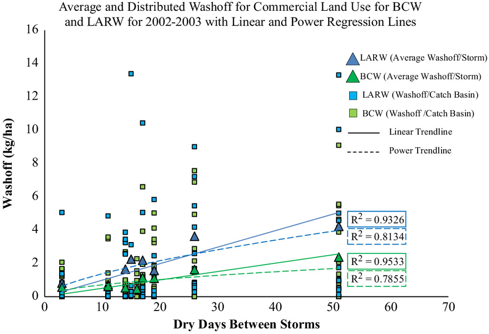
The washoff data from the LACBS shows an increased washoff load with an increasing number of dry days. A linear regression line and a power regression line were fit to the average washoff loads across all sites for each storm event. The intercept of the regression line was fixed at zero. This improved the linear correlation in some cases, and followed the framework of the SWMM reference manual (Rossman and Huber 2016). An example of this approach is shown in Fig. 2, with the coefficient of determination () for the trendlines. The washoff loads were analyzed against dry days in the program R, with a Pearson Correlation test, using the “cor.test” function from the “stats” package (R Core Team 2023). This determined that there is weak positive relationship () and the relationship is not significant (), when analyzing the washoff loads across all sites per storm event. However, when comparing the average washoff load across all sites against dry days, there is strong positive correlation () and the relationship is significant (). The same approach was implemented for all land uses for each year of sampling in both the LARW and the BCW.
Additional graphs for each land use type are provided in the Supplemental Materials. The values for all land uses are presented in the results section.
Washoff Parameter Development
Washoff parameters were developed to match observed data for individual storm events and the overall loading from a group of storm events, given changes in mean runoff. A constant buildup rate was desired to be used across multiple years for a given land use, so that the only variables affecting washoff load were the available buildup load, and rainfall-runoff for a given storm. Fig. 3 shows average washoff loads for all land uses, with both rainfall and buildup days before storm events plotted for both years of samplingwhere = rate of washoff (); = washoff coefficient (); = washoff exponent (unitless); = runoff rate per unit area (); and = pollutant buildup (kg).
(3)

When comparing events with similar simulated buildup, in some cases increased rainfall correlated with increased washoff. Other correlations that could have resulted in the deviations from the expected washoff loads are in the discussion section.
The washoff equation in SWMM has three different possible forms: exponential, rating curve, and event mean concentration (EMC). The EMC approach produces washoff concentrations that are uniform within-storm and the loading rate for the entire storm will vary in direct proportion to the runoff rate. By using either a rating curve or exponential function, washoff rates can be simulated to increase and decline proportional to storm runoff. The rating curve is typically used for natural catchments and rivers, where sediment load is proportional to flow raised to a power (Rossman and Huber 2016). Based on these criteria, the exponential washoff function [Eq. (3)] was chosen.
The parameters and were developed based on storm events with similar buildup days but different runoff rates per unit area. We assume that if buildup rates are constant, then two events with similar buildup days would have approximately the same buildup at the start of the storm, but the differences in observed washoff could be correlated to differences in rainfall. Using this assumption, Eq. (3) was rearranged to determine . For example, if a given runoff rate per unit area washed off only a percentage of the presumed available load, and a value for was selected based on the literature, then Eq. (3) could be used to determine . This method was used to provide an initial estimate of a possible value for and was adjusted further to match target loading during calibration.
Litter Loading Validation for LA County Watersheds
Two forms of validation were conducted for the LA County watersheds. The first analysis was conducted using the second year of data from the LACBS. These data were collected from 2003 to 2004 in the same manner as the previous year. A key factor was the reduction in rainfall for this validation year, which was approximately half of the previous year. Observed data were scaled up from the average values from LACBS, taking the average washoff/storm (), and multiplying it by the total land use area. Scaled-up values were used for comparison with simulated results. The second validation was conducted using data from the Ballona Creek Trash Interceptor, developed by The Ocean Cleanup. The Ballona Creek Trash Interceptor collected litter from the outlet of the Ballona Creek Watershed from October 2022 through May 2023. Data were published on their website and the total annual loading for the 2022–2023 wet season was used to validate the buildup and washoff parameters (The Ocean Cleanup 2023).
Hydrologic Verification and Litter Loading Validation for the Lower San Diego River Watershed
Two USGS stream gages were used to verify the hydrologic modeling in the LSDRW (Fig. 1). An upstream gage and downstream gage were used. Flow rate data were acquired from the USGS National Water Information System. These data were then imported into PCSWMM as a time series and compared with simulated results. A total of 13 rain events were used for hydrologic verification. The average value for the maximum (peak) flow of the 13 rain events was calculated and compared. These storms were within the time range used for litter loading validation (presented below).
Buildup and washoff parameters developed for the LA County watersheds were applied to the LSDRW and validated with data from a Technical Report by Michael Baker International, Regional Trash Generation Rates for Priority Land Uses in San Diego County (Michael Baker International 2018). Their research determined regional trash generation rates for priority land uses in San Diego County, which involved installing full capture devices in 36 drain inlets throughout the county. Collection from these drain inlets was conducted quarterly. After validating the LARW and BCW, the BCW parameters were used for the LSDRW, due to more recently available validation data. Simulated results were compared with observed data for each land use. Litter generation rates for each land use were scaled up in the same manner as the LA County watersheds to compare total simulated litter load with observed data.
Street Sweeping
Due to lack of data, street sweeping was excluded from the LARW and BCW PCSWMM models. Street sweeping is included in the LSDRW model, reducing the available buildup load. Within PCSWMM, a user can define a sweeping interval, buildup available for removal, and removal efficiency. Based on data from the City of San Diego, the street sweeping interval was set to be weekly. The buildup available was determined by estimating the area associated with roads in each land use type. A GIS shape file was used to determine the lengths of roads within each land use type, an average width was used to convert the lengths into an area. This average width (15 m) was based on information from the City of San Diego Transportation Manual (Millard-Ball 2022). A percentage of the total land use area that is roads is used as the buildup available to be swept. Lacking sufficient data on removal efficiencies for litter, three different scenarios were tested: 70%, 80%, and 90% removal efficiency (Selbig and Bannerman 2007). Street sweeping analyses were conducted in ideal scenarios where all streets that are capable of being swept are, meaning cars or other obstructions did not stop the sweeper.
Please see the Supplementary Materials for more information on sensitivity analysis, model calibration, and validation.
Results
Hydrologic Verification
Table 1 shows the verification of hydrologic data between simulated and observed data. Table 1 shows the values associated with the downstream (Fashion Valley) and upstream (Santee) USGS stream gages. The model was run with a continuous simulation from July 2016 to November 2017, and the following error functions were tested: Nash–Sutcliffe efficiency (NSE) and integral square error (ISE). NSE and ISE values were calculated for total inflow () between simulated and observed data. Depending on the NSE value, model performance is considered to be very good (), good (NSE between 0.65 and 0.75), satisfactory (NSE between 0.5 and 0.65), or unsatisfactory () (Moriasi et al. 2007; Pachepsky et al. 2016). ISE values are good if the value is between 6.0 and 10.0, very good if between 3.0 and 6.0, and excellent if less than 3.0 (Sarma et al. 1973). The relatively low percent error between observed and simulated average peak flow (), the NSE values in the very good (0.79) and satisfactory (0.54) ranges, and the excellent rating for ISE allow this verification to be satisfactory for hydrologic performance.
| Stream gage | Date range | Number of storm events | Observed average peak flow () | Simulated average peak flow () | % error between average peak flow | NSE | ISE |
|---|---|---|---|---|---|---|---|
| Fashion Valley | July 2016–Nov 2017 | 13 | 29.41 | 24.57 | 16 | 0.79 | 1.54 |
| Santee | 17.98 | 18.93 | 0.54 | 1.86 |
Buildup Parameter Comparison
The buildup rates () associated with the linear buildup function are presented in Table 2. The and buildup time exponent () associated with the power buildup function are also presented in Table 2. Initial maximum buildup values () values were taken as the greatest observed washoff load for each land use.
| Watershed | Sampling year | Land use | Maximum buildup possible | Linear buildup | Power buildup | |||
|---|---|---|---|---|---|---|---|---|
| () | () | () | ||||||
| LARW | 2002–2003 | Commercial | 4.2 | 0.099 | 0.93 | 0.35 | 0.65 | 0.95 |
| Residential | 0.96 | 0.025 | 0.56 | 0.048 | 0.78 | 0.04 | ||
| Industrial | 17.5 | 0.38 | 0.91 | 0.11 | 1.4 | 0.70 | ||
| Open space | 0.57 | 0.022 | 0.55 | 0.25 | 0.23 | 0.02 | ||
| BCW | 2002–2003 | Commercial | 2.7 | 0.056 | 0.95 | 0.24 | 0.52 | 0.66 |
| Residential | 0.85 | 0.016 | 0.85 | 0.11 | 0.33 | 0.20 | ||
| Industrial | 1.47 | 0.032 | 0.91 | 0.13 | 0.56 | 0.62 | ||
| Open space | 2.6 | 0.050 | 0.82 | 0.23 | 0.48 | 0.31 | ||
| LARW | 2003–2004 | Commercial | 2.7 | 0.062 | 0.88 | 0.39 | 0.47 | 0.74 |
| Residential | 0.73 | 0.021 | 0.69 | 0.097 | 0.53 | 0.95 | ||
| Industrial | 7.7 | 0.19 | 0.70 | 0.64 | 0.60 | 0.64 | ||
| Open space | 3.9 | 0.049 | 0.71 | 0.046 | 0.83 | 0.29 | ||
| BCW | 2003–2004 | Commercial | 1.1 | 0.018 | 0.94 | 0.15 | 0.45 | 0.95 |
| Residential | 0.97 | 0.019 | 0.84 | 0.26 | 0.30 | 0.98 | ||
| Industrial | 1.1 | 0.022 | 0.74 | 0.48 | 0.18 | 0.95 | ||
| Open space | 1.3 | 0.029 | 0.75 | 0.47 | 0.25 | 0.75 | ||
Values for linear buildup rates across all land use types ranged from 0.016 to , with a mean of . Values for power buildup rates ranged from 0.046 to 0.64 (mean of 0.25), and exponents in the range of 0.18 to 1.4 (mean 0.54). Maximum buildup values ranged from 0.57 to , with a mean of . Our mean buildup rates are slightly higher than those reported in BASMAA (2014), with a mean of and a maximum of . Winston et al. (2023) reported a buildup loading rate in the range of 0.10 to with a mean value of . Their higher values are impacted by the fact that approximately 80% of the collected material was natural litter (leaf litter, etc.).
Buildup/Washoff Calibration and Validation for LA County Watersheds
Based on our initial estimates from using Eq. (3), when was set to equal 0.5, ranged from 0.6 to 2.0, depending on which two storms with similar buildup periods were being analyzed. These initial values worked well to estimate washoff loads for some storm events, but over- or underestimated the values for others. Fig. 4 presents simulated washoff loading rate (kg/h) compared with observed data converted to (kg/h). Observed washoff data are presented as the total loading (kg) for a given storm and divided by the duration (h) of the simulated storm event. Table 3 provides additional context about the presented storm events in Fig. 4.
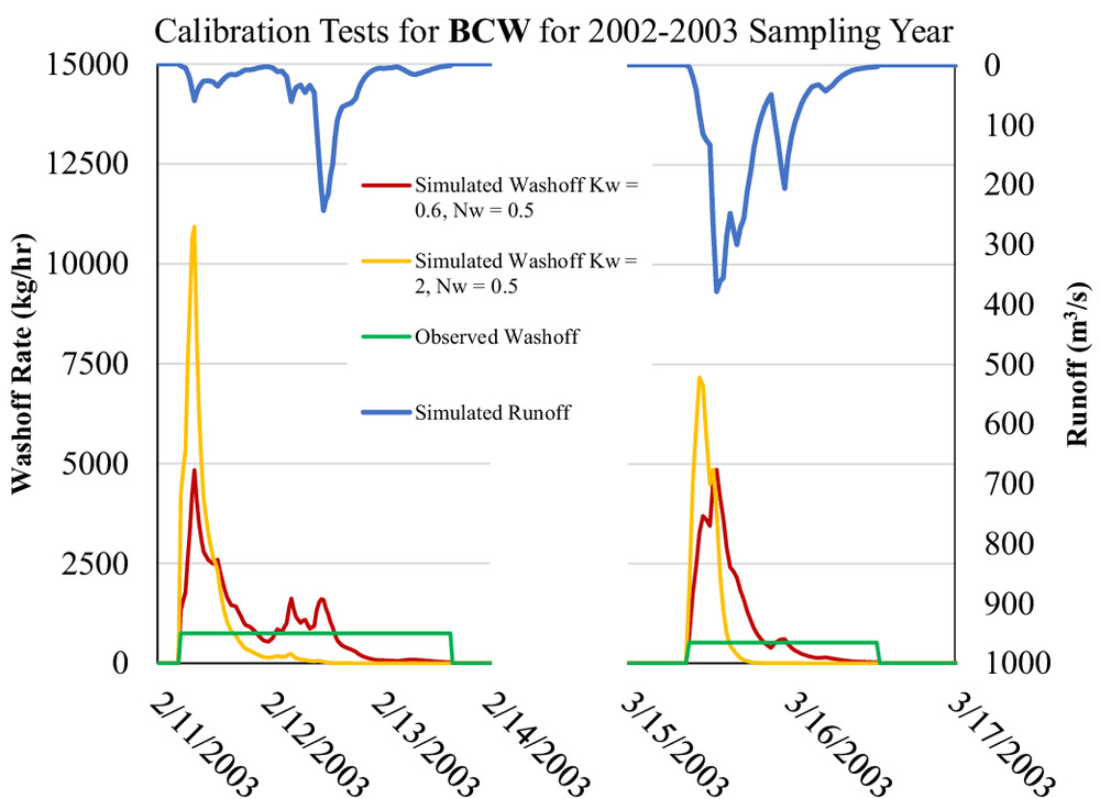
| Storm event | Antecedent dry days | Rainfall (mm) | Max rainfall intensity | Scenario | Washoff load (kg) |
|---|---|---|---|---|---|
| 2/11/2003–2/14/2003 | 50 | 91 | 12.20 | , | 52,596 |
| , | 55,510 | ||||
| Observed | 44,104 | ||||
| 3/15/2003–3/17/2003 | 17 | 108 | 21.59 | , | 30,659 |
| , | 25,570 | ||||
| Observed | 14,578 |
Large volumes of runoff and highest rainfall did not always produce large washoff loads. Runoff combined with a long period of dry weather resulted in the greatest washoff loads. Large washoff loads were also observed with relatively low rainfall when there was a longer period of dry weather (Alam et al. 2017).
The preliminary estimates for the washoff parameters were calibrated to match observed washoff for all land uses. The final values were selected as (1.25) and (0.925). Table 4 shows calibrated values for and for a linear buildup function, using a constant and . Table 5 shows the target value of washoff load (kg/ha) used for calibration, the simulated washoff load using calibrated values from Table 4, and the error between the annual loads. The decision to use a single set of parameters to define washoff for all land uses is elaborated in the discussion section. Table 6 shows validation of the calibrated buildup and washoff parameters when applied to the following year of data in the LA County Watersheds, where rainfall depth decreased by nearly half.
| Watershed | Land use | ||
|---|---|---|---|
| LARW | Commercial | 0.1 | 4.5 |
| Residential | 0.03 | 1.5 | |
| Industrial | 0.4 | 13 | |
| Open space | 0.025 | 3 | |
| BCW | Commercial | 0.09 | 2 |
| Residential | 0.02 | 1.25 | |
| Industrial | 0.05 | 2 | |
| Open space | 0.08 | 2.5 |
| Watershed and sampling year | Land use | Target (kg/ha) | Simulated (kg/ha) | % error |
|---|---|---|---|---|
| LARW | Commercial | 17.02 | 17.06 | 0.20 |
| 2002–2003 | Residential | 4.82 | 5.33 | 10.70 |
| Nov 10–May 5 | Industrial | 60.70 | 57.30 | 5.61 |
| Open space | 4.63 | 4.92 | 6.30 | |
| BCW | Commercial | 9.41 | 6.80 | 27.74 |
| 2002–2003 | Residential | 2.69 | 2.65 | 1.25 |
| Nov 10–May 5 | Industrial | 5.57 | 6.01 | 8.05 |
| Open space | 8.80 | 8.27 | 6.11 |
| Watershed and sampling year | Land use | Target (kg/ha) | Simulated (kg/ha) | % error |
|---|---|---|---|---|
| LARW | Commercial | 10.82 | 10.91 | 0.83 |
| 2003–2004 | Residential | 3.58 | 3.57 | 0.31 |
| Nov 3–April 4 | Industrial | 30.65 | 32.79 | 6.98 |
| Open space | 5.79 | 3.85 | 33.46 | |
| BCW | Commercial | 2.74 | 4.14 | 51.02 |
| 2003–2004 | Residential | 3.01 | 1.87 | 37.92 |
| Nov 3–March 4 | Industrial | 3.84 | 3.86 | 0.58 |
| Open space | 4.84 | 4.97 | 2.78 |
The constant washoff parameters estimated washoff more closely in the LARW compared to the BCW. By design, the model was set to produce less washoff load when runoff decreased. The highest error occurred when washoff loads increased during the second year. High error also occurred for commercial land use in the BCW. From year 1 to year 2, there was approximately a 70% decrease in washed-off litter for commercial land use. Model parameters were unable to simulate this decrease based on runoff alone, indicating that other factors may have reduced observed washoff. The washoff exponent was the most sensitive parameter (Table 7). The maximum buildup and washoff coefficients were classified as sensitive, where the buildup rate constant was moderately sensitive.
| Parameter | Modified Morris sensitivity value | Ranking |
|---|---|---|
| 1.29 (very sensitive) | 1 | |
| 0.83 (sensitive) | 2 | |
| 0.51 (sensitive) | 3 | |
| 0.19 (moderately sensitive) | 4 |
Regional Estimates of Litter Loading for LA County Watersheds from Simulations
Regional estimates of litter transported by stormwater can inform municipalities of the scale and method of collection needed to capture and reduce the amount of litter entering waterways. Regional estimates based on calibrated parameters are presented in Table 8. These estimates were developed based on simulations for the 2002–2004 sampling events conducted by LA County. Our results provide regional estimates based on the average rates of washed-off litter (kg/ha) from each storm across all sites observed in LA County.
| Watershed | Simulation year | Total load from PCSWMM (kg) | Total load based on LACBS (2004) (kg) | Total load per unit area from PCSWMM (kg/ha) | Total load per unit area based on LACBS (2004) () | Total runoff volume from PCSWMM () | Total rainfall for simulation year (mm) |
|---|---|---|---|---|---|---|---|
| BCW | 2002–2003 (Calibrated) | 155,145 | 155,568 | 4.6 | 4.63 | 28,588,000 | 417.1 |
| BCW | 2003–2004 (Validated) | 103,205 | 117,600 | 3.1 | 3.5 | 18,334,400 | 223.5 |
| LARW | 2002–2003 (Calibrated) | 2,486,808 | 2,548,800 | 11.5 | 11.8 | 237,182,300 | 404.5 |
| LARW | 2003–2004 (Validated) | 1,584,020 | 1,913,760 | 7.3 | 8.86 | 124,718,100 | 226.8 |
The values developed for the BCW were validated against an additional year because there was an available dataset from the Ballona Creek Trash Interceptor. The values developed for the 2002–2004 year produced washoff estimates that were 2.6 times greater than the collected trash loads for 2022–2023 year. Therefore, BCW parameters were recalibrated to match the data for the 2022–2023 year (Table 9). values from Table 4 were scaled down by approximately 70% to match annual load with observed data.
| Watershed | Simulation year | Updated buildup rate constants, | Total trash collected by Ballona Creek trash interceptor (kg) | Total load from PCSWMM with initial values (kg) | Total load from PCSWMM with calibrated values (kg) | Total rainfall for simulation year (mm) |
|---|---|---|---|---|---|---|
| BCW | October 2022–May 2023 | Commercial: 0.027 | 70,170 | 183,131 | 71,361 | 431.8 |
| Residential: 0.006 | ||||||
| Industrial: 0.015 | ||||||
| Open space: 0.024 |
Street Sweeping Analysis
Street sweeping was tested for the same simulation year as hydrologic verification and litter loading validation, with the following removal efficiencies: 70%, 80%, and 90%. These removal efficiencies can collect 21%, 23%, and 25% of the available surface buildup, respectively.
Results and Validation for Lower San Diego River Watershed
Using the updated values (Table 9) and the values for the BCW (Table 4), regional estimates for the LSDRW were simulated. Table 10 shows the results for the 2016–2017 simulation year compared with data from Michael Baker International (2018). The annual washoff values were converted from lbs/acre to kg/ha.
| Land use | PCSWMM simulation for LSDRW with street sweeping (July 2016–November 2017) (kg/ha) | San Diego County special study mean values for litter generation rates (July 2016–November 2017) (kg/ha) | San Diego County special study maximum values for litter generation rates (July 2016–November 2017) (kg/ha) |
|---|---|---|---|
| Commercial | 4.48 | 1.1 | 4.3 |
| Industrial | 3.7 | 0.73 | 5.0 |
| Residential | 1.3 | 0.53 | 2.7 |
| Total | 2.15 | 0.77 | 3.56 |
The sample size for the validation is relatively low () and the distribution of sample sites does not fully represent the entire LSDRW watershed. These are some factors that could affect the validation. Other factors not captured in the model—such as topography, population density, climatic conditions such as wind, and the volume of vehicle and pedestrian traffic—can also impact the litter loading in an urbanized watershed.
The annual loading rates determined for the LSDRW fall within the range presented in BASMAA (2014). BASMAA (2014) estimates a production of litter of 0.5 to 150 (gallons/acre/year), which converts to approximately 0.38 to , depending on the land use and the median household income level (conversion made using their relationship of 0.68 lbs to each gallon of material). They split these estimates into low, moderate, high, and very high categories. Our estimation for the LSDRW for the year of July 2016 to November 2017 is . This falls in the range of the low estimate for the Bay Area, where low is less than , moderate is , and high estimates are . Alam et al. (2017) reported total pollutant load for wet seasons with the following values (): 4.5 (), 0.7 (), 3.7 (), 3.5 (). Weideman et al. (2020) quantified litter loading as for industrial land use, in commercial areas, and for residential areas. This equates to an annual loading of for industrial, for commercial, and for residential. The values for industrial and commercial land uses are much higher than our estimated loading for the LSDRW; however, the value for residential land use is only slightly higher than our estimated loading.
Discussion
Model parameters are uncertain because multiple values are needed to estimate them, and agencies may only collect data for some of the necessary values. Lacking knowledge of the initial or remaining buildup after storm events, it was difficult to develop washoff parameters. To develop more accurate washoff parameters, information is needed on the amount and material of available buildup at the start of a storm and residual buildup after a storm, to determine the effectiveness of a given rainfall-runoff to remove available litter load. A further investigation is also needed to assess the deposition of litter by other sources such as wind or direct dumping. LA County reported high litter loads in the storm drain outlets during the dry season, so litter is ending up in the storm system without runoff. This is not reflected in the present model.
There are contradictory findings related to correlation of rainfall-runoff and the amount of litter that is washed off in an urban catchment. In BAASMA (2014), washed-off trash did not correlate with rainfall intensity, runoff, or duration. This could indicate that buildup rates may vary throughout the year—i.e., buildup rates may be different in winter than in spring. If litter washoff is not strongly correlated with rainfall-runoff, then developing washoff parameters to estimate annual loading may not be the best method. Instead, buildup rates could vary, and once a threshold value of runoff is met, then the total available load is washed off. On the contrary, Winston et al. (2023) found that rainfall depth, duration, and peak rainfall intensity were significantly correlated to either macrodebris mass or volume. In the LA County washoff data, there is a clear reduction in rainfall-runoff and reduction in washoff load for both watersheds in the second year. This may reveal some correlation between rainfall-runoff quantities and washed off litter.
We developed washoff parameters from storm events with similar antecedent dry days where runoff correlated with washoff load. This assumption works well if the objective is to match total annual washoff loads. However, it does not work well if the objective is to assess the transportability of trash with respect to different rainfall intensities for select storm events. We assume that litter is generally composed of the same materials across watersheds; therefore, we use a single set of washoff parameters for all land uses. A more accurate approach would be to define varying washoff parameters based on the materials associated with the litter from specific land uses. This would require an understanding of the typical density of each litter material and a more refined distribution of subcatchments in the PCSWMM model (i.e., each subcatchment would need to have only one land use).
Our simulation results suggest there is the potential to use washoff data at small catchment scales to estimate regional litter loading based on the relative similarity between final estimates with LA County. However, when applying parameters from one watershed to another, extensive data are needed for calibration and validation data. The calibration data are needed to adjust the washoff parameters, and the remaining data are needed to validate that the model reflects the conditions of the watershed. Additional litter may enter a watershed through direct deposition and storage in larger floodplains downstream of the small drainages monitored in the current available datasets. The washoff parameters could also be further optimized to more accurately represent the effectiveness of a given storm to washoff available litter.
Conclusion and Future Work
We demonstrate the potential to develop standardized buildup and washoff parameters for urbanized watersheds. This work is aimed at improving estimates of litter loading from various land uses. Antecedent dry days were found to be a strong control on litter loads, and rainfall and runoff also impacted litter loads. Our model does not fully evaluate the impact of direct dumping; direct dumping could result in some of the unexplained large spikes of washed-off litter. We found the implementation of maximum buildup values effective to match simulated and observed data for multiyear simulations and constant parameter values. Standardizing these parameters would allow for efficient estimations of litter loading based on readily available land use information.
Simulated litter generation rates in the BCW and LSDRW varied by about 2 to 5 times when compared to validation data from different years. This indicates that other factors must be considered when applying buildup and washoff parameters from one watershed to another (population density, climatic conditions, socioeconomic data, demographics, site visitation, and vehicular traffic). A pure modeling approach does not fully account for this variability because average values are used when setting maximum buildup values and calculating buildup rates. Additional field data can supplement the findings from our modeled results to model and manage litter more effectively. Ultimately, long-term datasets are needed to improve model performance. Field measurements that focus on areas where there were the greatest observed unexplained spikes in washed-off litter could determine if these spikes are truly outliers or if there is a trend of factors—such as location or socioeconomic factors—leading to an increase in litter spikes. These potential outliers can be seen in the Supplemental Materials related to the washoff loads across all sites per land use in the LARW and BCW. A deeper assessment of socioeconomic factors in certain areas would provide a better understanding of the factors contributing to trash generation. Similarly, dividing the residential category into its various subgroups, such as multifamily, would improve the accuracy of modeled results.
Supplemental Materials
File (supplemental materials_joeedu.eeeng-7474_bagheri.pdf)
- Download
- 1.44 MB
Data Availability Statement
All software and data can be made available upon request from the corresponding author.
Acknowledgments
This project was funded by the NOAA Marine Debris Program, award NA21NOS9990109. Thank you also to PCSWMM for their support of an educational research grant that made this project possible. The development of the computer model was also partially supported by NSF Award No. 2244837.
References
Alam, M. Z., A. Anwar, A. Heitz, and D. C. Sarker. 2018. “Improving stormwater quality at source using catch basin inserts.” J. Environ. Manage. 228 (Jan): 393–404. https://doi.org/10.1016/j.jenvman.2018.08.070.
Alam, M. Z., A. H. M. F. Anwar, D. C. Sarker, A. Heitz, and C. Rothleitner. 2017. “Characterising stormwater gross pollutants captured in catch basin inserts.” Sci. Total Environ. 586 (Feb): 76–86. https://doi.org/10.1016/j.scitotenv.2017.01.210.
Alley, W. M., and P. E. Smith. 1981. “Estimation of accumulation parameters for urban runoff quality modeling.” Water Resour. Res. 17 (6): 1657–1664. https://doi.org/10.1029/WR017i006p01657.
Armitage, N. 2007. “The reduction of urban litter in the stormwater drains of South Africa.” Urban Water J. 4 (3): 151–172. https://doi.org/10.1080/15730620701464117.
Armitage, N., and A. Rooseboom. 2000. “The removal of urban litter from stormwater conduits and streams: Paper 1-The quantities involved and catchment litter management options.” Water SA 26 (2): 181–188.
BASMAA (Bay Area Stormwater Management Agencies Association). 2011. Technical memorandum #1- Summary of techniques used to quantify trash in stormwater, a conceptual model of trash loading, and a method for establishing baseline loads. Oakland, CA: EOA.
BASMAA (Bay Area Stormwater Management Agencies Association). 2014. San Francisco Bay area stormwater trash generation rates. Oakland, CA: EOA.
Bonhomme, C., and G. Petrucci. 2017. “Should we trust build-up/wash-off water quality models at the scale of urban catchments?” Water Res. 108 (Jan): 422–431. https://doi.org/10.1016/j.watres.2016.11.027.
Boroon, M., and C. Coo. 2015. “Water quality assessment of the Los Angeles river watershed, California, USA in wet and dry weather periods.” J. Geogr. Environ. Earth Sci. Int. 3 (4): 1–17. https://doi.org/10.9734/JGEESI/2015/20717.
California Regional Water Quality Control Board Los Angeles Region. 2001. Trash total maximum daily loads for the Ballona Creek and wetland. Los Angeles: California Regional Water Quality Control Board Los Angeles Region.
Chaudhary, S., L. H. Chua, and A. Kansal. 2021. “Modeling washoff in temperate and tropical urban catchments.” J. Hydrol. 603 (Apr): 126951. https://doi.org/10.1016/j.jhydrol.2021.126951.
Chen, Y., C. Gu, C. Shao, and X. Qin. 2019. “Parameter sensitivity and inversion analysis for a concrete face rockfill dam based on CS-BPNN.” Adv. Civ. Eng. 2019 (Feb): 9742961. https://doi.org/10.1155/2019/9742961.
Conley, G., S. C. Zinn, T. Hanson, K. McDonald, N. Beck, and H. Wen. 2022. “Using a deep learning model to quantify trash accumulation for cleaner urban stormwater.” Comput. Environ. Urban Syst. 93 (Apr): 101752. https://doi.org/10.1016/j.compenvurbsys.2021.101752.
County of Los Angeles Department of Public Works Watershed Management Division. 2004. Trash baseline monitoring results Los Angeles River and Ballona Creek watershed. Los Angeles: County Los Angeles.
Geosyntec Consultants. 2016. The City of San Diego Stormwater standards. San Diego: City of San Diego.
Gold, M., T. Hogue, S. Pincetl, K. Mika, and K. Radavich. 2015. Los Angeles sustainable water project: Ballona Creek watershed (full report). Los Angeles: UCLA Grand Challenges.
Hadiuzzaman, M., M. Salehi, and T. Fujiwara. 2022. “Plastic litter fate and contaminant transport within the urban environment, photodegradation, fragmentation, and heavy metal uptake from storm runoff.” Environ. Res. 212 (Aug): 113183. https://doi.org/10.1016/j.envres.2022.113183.
Hao, X., Y. Li, and S. Liu. 2021. “Comparison of dynamic flow interaction methods between pipe system and overland in urban flood analysis.” Sci. Rep. 11 (1): 12079. https://doi.org/10.1038/s41598-021-88246-z.
Holt, B., R. Trinh, and M. M. Gierach. 2017. “Stormwater runoff plumes in the Southern California Bight: A comparison study with SAR and MODIS imagery.” Mar. Pollut. Bull. 118 (1–2): 141–154. https://doi.org/10.1016/j.marpolbul.2017.02.040.
Hong, Y., Q. Liao, C. Bonhomme, and G. Chebbo. 2019. “Physically-based urban stormwater quality modelling: An efficient approach for calibration and sensitivity analysis.” J. Environ. Manage. 246 (Jan): 462–471. https://doi.org/10.1016/j.jenvman.2019.06.003.
Hossain, I., M. Imteaz, S. Gato-Trinidad, and A. Shanableh. 2010. “Development of a catchment water quality model for continuous simulations of pollutants build-up and wash-off.” Int. J. Civ. Environ. Eng. 1 (1): 210–217.
Hossain, I., M. A. Imteaz, and M. I. Hossain. 2012. “Application of a catchment water quality model for an East-Australian catchment.” Int. J. Global Environ. Issues 12 (2–4): 242–255. https://doi.org/10.1504/ijgenvi.2012.049370.
Kim, L.-H. 2002. Monitoring and modeling of pollutant mass in urban runoff: Washoff, buildup and litter. Los Angeles: Univ. of California.
Kim, L.-H., and J. Kang. 2004. “Loading rates and characteristics of litter from highway stormwater runoff.” J. Korean Soc. Water Environ. 20 (5): 415–421.
Kim, L.-H., M. Kayhanian, and M. K. Stenstrom. 2004. “Event mean concentration and loading of litter from highways during storms.” Sci. Total Environ. 330 (1): 101–113. https://doi.org/10.1016/j.scitotenv.2004.02.012.
Lehtinen, S. 2014. “Simulation of stormwater quality in an urban catchment using the Stormwater Management Model (SWMM).” Master’s thesis, School of Chemical Technology, Degree Programme of Chemical Technology.
Li, C., M. Liu, Y. Hu, J. Gong, and Y. Xu. 2016. “Modeling the quality and quantity of runoff in a highly urbanized catchment using storm water management model.” Pol. J. Environ. Stud. 25 (4): 1573–1581.
Li, J., C. Mu, C. Deng, and M. Ma. 2020. “Hydrologic-environmental effects of sponge city under different spatial scales.” J. Water Reuse Desalin. 10 (1): 45–56. https://doi.org/10.2166/wrd.2019.046.
Liang, X., M. H. Park, and M. K. Stenstrom. 2019. “Socio-economic factors of high trash generation in the city of Los Angeles.” Water Sci. Technol. 80 (3): 408–417. https://doi.org/10.2166/wst.2019.283.
Los Angeles County Public Works. 2023a. “Ballona Creek Watershed.” Accessed October 18, 2023. https://dpw.lacounty.gov/wmd/watershed/bc/.
Los Angeles County Public Works. 2023b. “Los Angeles River watershed.” Accessed October 18, 2023. https://dpw.lacounty.gov/wmd/watershed/LA/.
Ma, K.-C., M.-H. Chuang, and T.-Y. Chan. 2021. “Analysis of flooding adaptation and groundwater recharge after adopting JW ecological technology in a highly developed urbanization area.” Appl. Sci. 11 (6): 2662. https://doi.org/10.3390/app11062662.
Martin, C., Q. Zhang, D. Zhai, X. Zhang, and C. M. Duarte. 2021. “Enabling a large-scale assessment of litter along Saudi Arabian red sea shores by combining drones and machine learning.” Environ. Pollut. 277 (Jan): 116730. https://doi.org/10.1016/j.envpol.2021.116730.
Martinez, E., and R. Griffiths. 2023. Vol. 110 of Assessing litter loads and composition from urban stormwater discharges in Northland. Whangārei, New Zealand: Northland Regional Council.
Michael Baker International. 2018. Regional trash generation rates for priority land uses in San Diego County. Carlsbad, CA: Michael Baker International.
Millard-Ball, A. 2022. “The width and value of residential streets.” J. Am. Plann. Assoc. 88 (1): 30–43. https://doi.org/10.1080/01944363.2021.1903973.
Mohammed, M. H., H. M. Zwain, and W. H. Hassan. 2022. “Modeling the quality of sewage during the leaking of stormwater surface runoff to the sanitary sewer system using SWMM: A case study.” AQUA—Water Infrastruct. Ecosyst. Soc. 71 (1): 86–99.
Moore, S., M. Sutula, T. Von Bitner, G. Lattin, and K. Schiff. 2016. Southern California bight 2013 regional monitoring program: Volume III. Trash and marine debris. Costa Mesa, CA: Southern California Coastal Water Research Project Costa Mesa (CA).
Moriasi, D. N., J. G. Arnold, M. W. Van Liew, R. L. Bingner, R. D. Harmel, and T. L. Veith. 2007. “Model evaluation guidelines for systematic quantification of accuracy in watershed simulations.” Trans. ASABE 50 (3): 885–900. https://doi.org/10.13031/2013.23153.
NRCS (Natural Resources Conservation Service). n.d. “Web soil survey.” Accessed October 18, 2023. https://websoilsurvey.nrcs.usda.gov/.
Pachepsky, Y., G. Martinez, F. Pan, T. Wagener, and T. Nicholson. 2016. “Evaluating hydrological model performance using information theory-based metrics.” Hydrol. Earth Syst. Sci. Discuss. 1–24. https://doi.org/10.5194/hess-2016-46.
Peng, J., L. Yu, Y. Cui, and X. Yuan. 2020. “Application of SWMM 5.1 in flood simulation of sponge airport facilities.” Water Sci. Technol. 81 (6): 1264–1272. https://doi.org/10.2166/wst.2020.221.
Prata, J. C., J. P. da Costa, I. Lopes, A. C. Duarte, and T. Rocha-Santos. 2020. “Environmental exposure to microplastics: An overview on possible human health effects.” Sci. Total Environ. 702 (Feb): 134455. https://doi.org/10.1016/j.scitotenv.2019.134455.
Project Clean Water. 2022. “San Diego River.” Accessed October 18, 2023. https://projectcleanwater.org/watersheds/san-diego-river-wma/.
R Core Team. 2023. R: A language and environment for statistical computing. Vienna, Austria: R Foundation for Statistical Computing.
Rossman, L. A., and W. C. Huber. 2016. Storm water management model reference manual—Water quality. Washington, DC: Office of Research and Development.
Sarma, P., J. Delleur, and A. Rao. 1973. “Comparison of rainfall-runoff models for urban areas.” J. Hydrol. 18 (3–4): 329–347. https://doi.org/10.1016/0022-1694(73)90056-5.
Sartor, J. D., G. B. Boyd, and F. J. Agardy. 1974. Water pollutant aspects of street surface contaminants. Washington, DC: USEPA.
Selbig, W. R., and R. T. Bannerman. 2007. Evaluation of street sweeping as a stormwater-quality-management tool in three residential basins in Madison, Wisconsin. Reston, VA: USGS.
Sun, X. Y., L. T. H. Newham, B. F. W. Croke, and J. P. Norton. 2012. “Three complementary methods for sensitivity analysis of a water quality model.” Environ. Modell. Software 37 (Feb): 19–29. https://doi.org/10.1016/j.envsoft.2012.04.010.
Tetra Tech. 2010. Stormwater best management practices (BMP) performance analysis. Fairfax, VA: Tetra Tech.
The Ocean Cleanup. 2023. “Los Angeles County Ballona Creek trash interceptor pilot project.” Accessed October 18, 2023. https://ballonainterceptor.lacounty.gov/.
Tu, M.-C., and P. Smith. 2018. “Modeling pollutant buildup and washoff parameters for SWMM based on land use in a semiarid urban watershed.” Water Air Soil Pollut. 229 (4): 5. https://doi.org/10.1007/s11270-018-3777-2.
Tuomela, C., N. Sillanpää, and H. Koivusalo. 2019. “Assessment of stormwater pollutant loads and source area contributions with storm water management model (SWMM).” J. Environ. Manage. 233 (Apr): 719–727. https://doi.org/10.1016/j.jenvman.2018.12.061.
Vanrolleghem, P. A., G. Mannina, A. Cosenza, and M. B. Neumann. 2015. “Global sensitivity analysis for urban water quality modelling: Terminology, convergence and comparison of different methods.” J. Hydrol. 522 (Aug): 339–352. https://doi.org/10.1016/j.jhydrol.2014.12.056.
Weideman, E. A., V. Perold, G. Arnold, and P. G. Ryan. 2020. “Quantifying changes in litter loads in urban stormwater run-off from Cape Town, South Africa, over the last two decades.” Sci. Total Environ. 724 (Feb): 138310. https://doi.org/10.1016/j.scitotenv.2020.138310.
Wicke, D., T. A. Cochrane, and A. O’Sullivan. 2012. “Build-up dynamics of heavy metals deposited on impermeable urban surfaces.” J. Environ. Manage. 113 (Aug): 347–354. https://doi.org/10.1016/j.jenvman.2012.09.005.
Winston, R. J., J. D. Witter, R. A. Tirpak, L. Sester, H. Jenkins, and V. Lillard. 2023. “Abundance and composition of anthropogenic macrolitter and natural debris in road runoff in Ohio, USA.” Water Res. 239 (Mar): 120036. https://doi.org/10.1016/j.watres.2023.120036.
Zhong, B., Z. Wang, H. Yang, H. Xu, M. Gao, and Q. Liang. 2023. “Parameter optimization of SWMM model using integrated Morris and GLUE methods.” Water 15 (1): 149. https://doi.org/10.3390/w15010149.
Information & Authors
Information
Published In

Journal of Environmental Engineering
Volume 150 • Issue 8 • August 2024
Copyright
This work is made available under the terms of the Creative Commons Attribution 4.0 International license, https://creativecommons.org/licenses/by/4.0/.
History
Received: Jun 13, 2023
Accepted: Jan 29, 2024
Published online: May 25, 2024
Published in print: Aug 1, 2024
Discussion open until: Oct 25, 2024
ASCE Technical Topics:
- Calibration
- Design (by type)
- Engineering fundamentals
- Environmental engineering
- Infrastructure
- Load factors
- Mathematics
- Measurement (by type)
- Parameters (statistics)
- Pollutants
- River engineering
- River systems
- Rivers and streams
- Solid wastes
- Statistics
- Structural design
- Urban and regional development
- Urban areas
- Wastes
- Water and water resources
- Watersheds
Authors
Metrics & Citations
Metrics
Citations
Download citation
If you have the appropriate software installed, you can download article citation data to the citation manager of your choice. Simply select your manager software from the list below and click Download.