Evaluation of Hydrodynamic Mixing in an Afterbay Reservoir
Publication: Journal of Environmental Engineering
Volume 149, Issue 10
Abstract
This study focused on the mixing of a solute, assumed to be conservative, introduced to one arm of an afterbay reservoir, between Keswick and Shasta Dams on the Sacramento River near Redding, California. Rhodamine water tracer (WT) dye served as the solute in a field experiment, and was introduced over 4.5 h and monitored for 4 days by sondes moored in the reservoir. The scenario was modeled numerically using the Delft3D flexible mesh (FM) hydrodynamic and mixing model, with measured inflows, outflows, water level, water temperatures, and bathymetry as input. Manning’s and horizontal eddy viscosity served as the (constant) model calibration parameters, and each was adjusted an order of magnitude below the default values to force observed and modeled dye hydrographs to match in arrival time and duration. The low friction factor was concluded to be due to a combination of low flow speeds coupled with energy dissipation inherent to the model. The model and surface drifters equipped with dual-frequency Global Navigation Satellite System equipment revealed velocities in the range in much of the domain during the experiment. Simple analytical expressions were shown to be useful for estimating distance to full cross-sectional mixing, steady-state concentrations, and time to reach them, but the numerical model is required for investigation of the approach to steady state, and at locations where flows intersect. Time to steady-state concentrations was 1.5–13 days for 10 simulations that spanned a wide range of inflow conditions. Model sensitivity tests suggest that wind and heat fluxes were not important during the field study, but simulations of a summer scenario with small inflows of cold water upstream in warm weather should consider water temperature. Both field observations and numerical model results showed inflow to one arm of the reservoir reaching full cross-sectional mixing before plunging below the water surface near the intersection of this arm with the reservoir’s main stem. Model results are being used to guide management decisions related to inflows to the reservoir from a relic mining site that is also a USEPA Superfund site.
Introduction
Surface-water reservoirs typically are constructed to facilitate a combination of water supply, flood protection, power generation, and recreation goals. In many cases, reservoir water inflows also deliver contaminants, either in solution or sorbed onto particles transported in suspension or as bed load, often with associated environmental and human health concerns (Lemly 1997; Brenner et al. 2004). After the contaminant transport problem has been identified, common strategies for dealing with it include reducing concentrations at the source, impounding water upstream of the receiving water body, or diluting inflows with cleaner water (Nordstrom et al. 1999; Nordstrom and Alpers 1999; Turunen et al. 2020).
Many relic mining sites deliver contaminants to downstream waters: directly, as surface-water inflow; indirectly, as groundwater seepage; or both (Runkel et al. 2009). The fate of the contaminants can be investigated using periodic in situ sampling, or in some cases using automated data collection, the latter of which typically provides much higher temporal resolution. Many mixing and transport studies have been conducted using natural or introduced tracers (Wilson 1968; Wilson et al. 1986; Bencala et al. 1987; Kilpatrick and Wilson 1989; Kimball et al. 2002; Cowie et al. 2014). Field-based studies do not allow investigation of the efficacy of mitigation schemes until after they have been implemented, however.
A numerical model that describes both hydrodynamics and contaminant transport can provide results with high temporal and spatial resolution, and allows for simulation of multiple mitigation schemes and extreme events that have not yet occurred (Cole and Wells 2015; Chen et al. 2018; Park and Seo 2018). Multiple model runs can be performed to investigate the sensitivity of the problem to various inputs and calibration parameters, and to quantify statistics of output variables of interest.
Simulation of the fate of contaminants that react or evolve on timescales shorter than those of the transport processes being considered is more complicated than investigations of conserved contaminants because of the need to include source, sink, and growth or decay terms for the contaminant in the model (Amorim et al. 2021). These terms often are dependent on the concentration of the contaminant of interest or other substances, water chemistry, and environmental variables such as water temperature, air temperature, or solar radiation. In this case it may be necessary to run another model to provide input to the hydrodynamic mixing model. The source and sink terms also may include coefficients that are poorly known or unmeasured (Fischer et al. 1979).
This paper describes field-based and numerical modeling investigations of the mixing of a conserved solute within Keswick Reservoir, an afterbay reservoir on the Sacramento River in California. Particular focus was placed on how dilution varies with distance downstream, time, and inflow hydrographs. Reservoir inflows and outflows at the site are highly regulated, and one inflow is particularly concerning, from a water quality perspective, because it carries mineral mine runoff (Nordstrom et al. 1990; Alpers et al. 2000). This study included a field campaign to investigate the fate of Rhodamine WT dye introduced to this source, and a numerical modeling component that involved the use of the Delft3D FM v2022.04 hydrodynamic and transport model (Deltares 2021a, b) to simulate the stage, velocity, temperature, and concentration of a conserved contaminant throughout a range of operating conditions. This was done to provide information to a regulatory agency with oversight of reservoir water quality, to facilitate management decisions.
Site Description
The Sacramento River is the largest river in California, and is a critical component of the water resources infrastructure of the state, extending 400 km from its headwaters near the California–Oregon border to its junction with the San Francisco Estuary downstream. Shasta Lake, near the upstream end of the Sacramento River, is the largest surface-water reservoir in the state, at over 5.6 cubic kilometers at full pool, and its outflow passes through Keswick Reservoir and then downstream to meet ecological, municipal, industrial, and agricultural water needs of much of the rest of the state. Flow quantity and quality in the watershed, including water temperature, are intensely monitored and modeled for management purposes (Northern California Water Association 2006).
Keswick Reservoir (Fig. 1), 22 km in length, 50–200 m in breadth, and with maximum depth of approximately 30 m, lies within a steep canyon of the Sacramento River, with Shasta Dam defining the reservoir’s upstream extent and Keswick Dam defining its downstream limit. In normal operation, Shasta Dam outflow is adjusted to meet daily power demands, and Keswick Reservoir, two orders of magnitude smaller in volume than Shasta Lake, is operated as an afterbay, with Keswick Reservoir water level fluctuating as outflow remains relatively steady.
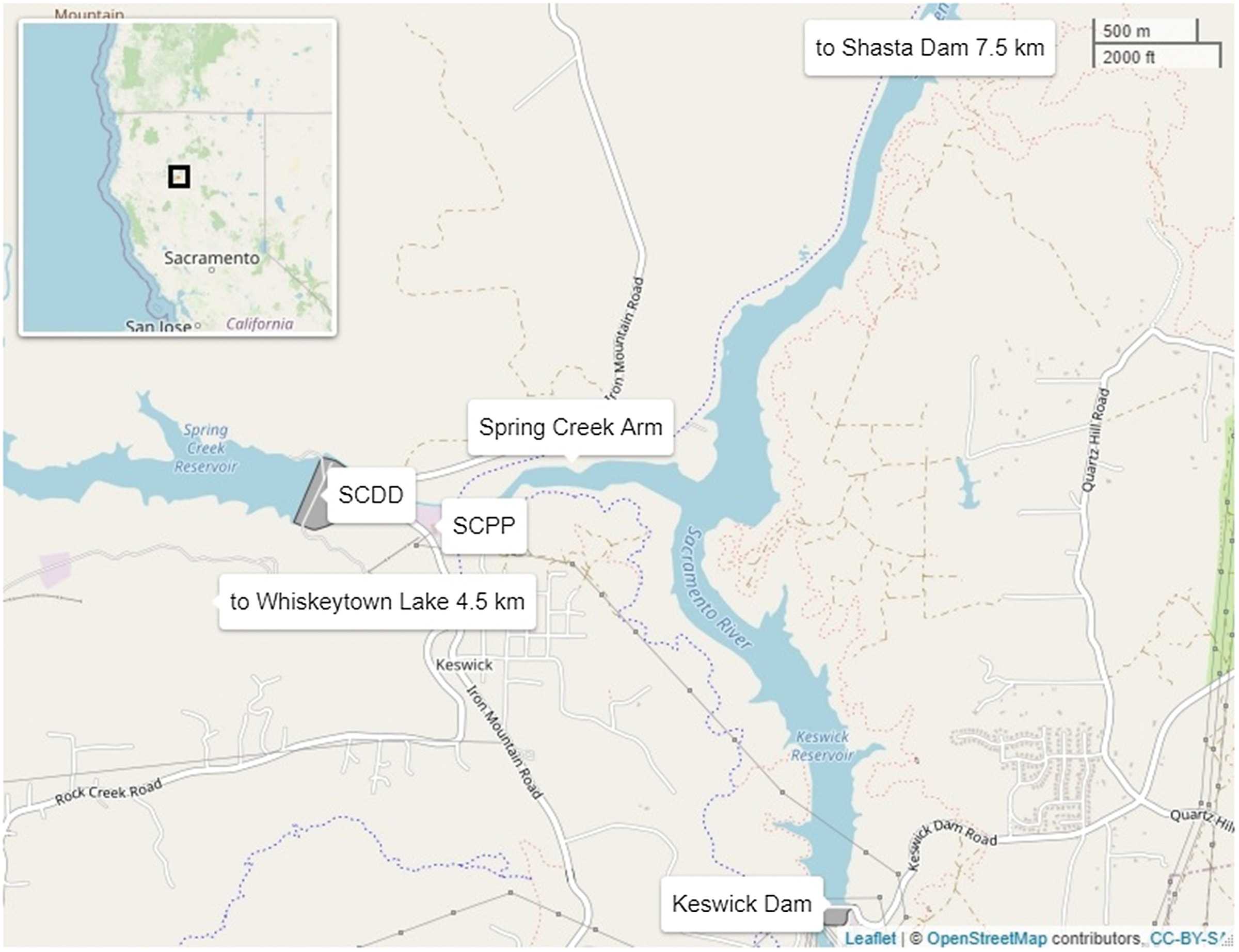
One tributary to Keswick Reservoir, Spring Creek, is dammed by the Spring Creek Debris Dam (SCDD) to trap treated outflow from the Iron Mountain Mine site, forming Spring Creek Reservoir (Fig. 1). SCDD is regulated manually to provide both a settling pond for contaminants and sufficient storage to contain mine runoff in the event of a storm. The Spring Creek Reservoir water level is drawn down periodically to provide capacity to capture future storms.
The Spring Creek Arm of Keswick Reservoir also receives water from nearby Whiskeytown Lake, as it passes through the Spring Creek Power Plant (SCPP) (Fig. 1). Thus there are three regulated inflows to Keswick Reservoir—at Shasta Dam, SCDD, and SCPP—and one outflow, at Keswick Dam. All four of these flowrates are controlled and monitored by the Bureau of Reclamation (henceforth, Reclamation). These flows define more than 90% of the water budget for Keswick Reservoir; the remainder is attributable to delivery by small (unmeasured) tributaries and rainfall directly onto the reservoir surface.
The USEPA lists zinc, copper, and cadmium as the metals that are of greatest concern for entry into Keswick Reservoir. Contaminants impact both water and sediment quality at the site (Nordstrom et al. 1999). The EPA funds periodic water sample collection to monitor water quality, and Reclamation routinely collects data defining the water budget and, at some locations, water temperature.
Data Collection for Model Input and Calibration
The investigation of mixing processes in Keswick Reservoir was designed primarily as a numerical modeling study, with a companion field campaign to acquire data needed for model calibration and subsequent simulations. The field work included bathymetric surveying, deployment of moored water quality sondes to record the time-dependent concentration of Rhodamine WT dye introduced to the Spring Creek Arm as a tracer, and Global Navigation Satellite System (GNSS)-equipped surface drifters to record surface flow pathlines.
Bathymetric Survey Data
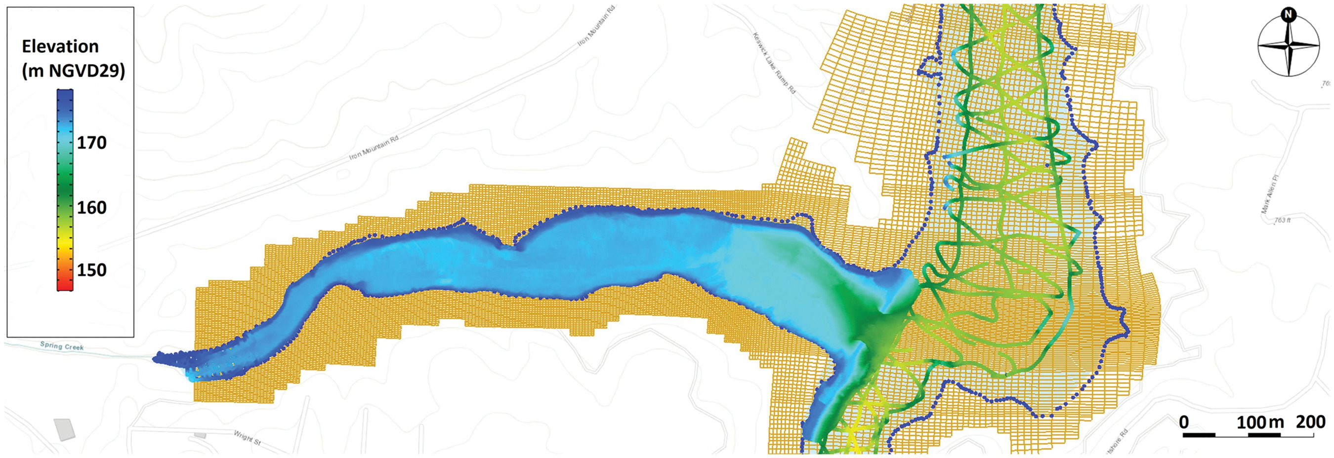
Surveys from 2010, 2016, and 2021 were used to define bathymetry of the reservoir, based on the assumption that bathymetry did not evolve over this period. The 2010 multibeam survey, performed by eTrac/AIS Construction, spanned most of the Spring Creek Arm, and only this region, whereas the 2016 single-beam survey (Deas and Sogutlugil 2017) omitted most of this region but included the rest of the reservoir, at lower resolution. Unfortunately, the vertical datum was unclear in both surveys. Likewise, the vertical datum for the Reclamation water level data for Keswick Reservoir is unknown. It was assumed that the vertical datum for both the 2010 survey and the water level data was the National Geodetic Vertical Datum of 1929 (NGVD29). After comparing the overlapping regions of the 2010 and 2016 surveys, the latter was adjusted uniformly upward by 0.35 m to force the two surveys to match within this region. The 2021 survey (Work 2022), performed using a Sontek M9 acoustic Doppler profiler (San Diego), targeted the extreme upstream end of the Spring Creek Arm of the reservoir, which previously was unsurveyed. The 2021 survey also was adjusted upward, by 0.45 m, to force it to match the 2010 survey, where they overlapped.
GNSS equipment was used for horizontal position data in each survey. Information regarding uncertainty of the 2010 and 2016 data sets is not available. The 2021 data set has depths with decimeter-level uncertainty, and meter-level uncertainty in horizontal position. Fig. 2 shows the footprint of the three surveys.
Reservoir Inflows and Outflows
Flows through Keswick Dam and SCPP are measured by acoustic travel-time flowmeters mounted in steel pipelines, and data are recorded hourly by Reclamation. Flow through Shasta Dam is computed based on electric power production. Reclamation computes net inflow to Keswick Reservoir using measured inflows, outflow, and water level changes, and reports results hourly.
A lookup table is used to define the degree to which the gate at SCDD should be opened to achieve a given desired discharge for a given amount of head in Spring Creek Reservoir. The flow exiting the dam passes through a V-notch weir that has a labeled gauge on it to indicate both head on the weir and discharge. Discharge was measured independently by towing a floating acoustic Doppler current profiler across the weir section seven times during two different days, when the Reclamation-reported discharge was . It was concluded that the gauge printed on the weir is correct and that the discharge reported by Reclamation was high by 9% for the observed flow conditions. As a result, all discharges from SCDD reported by Reclamation were derated by 9%. This is important because it was this flow that received the introduced Rhodamine WT dye.
Dye Introduction
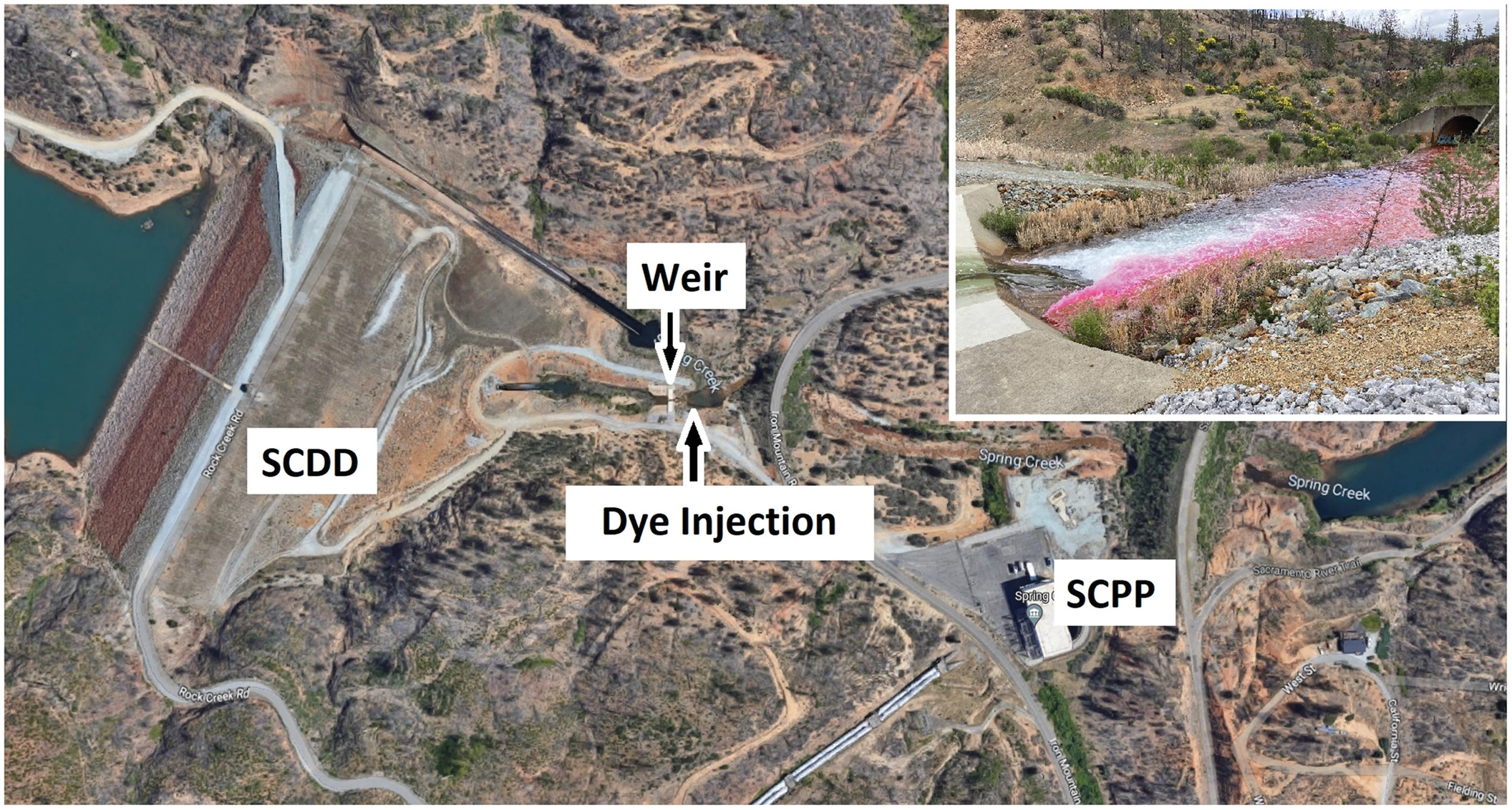
A simple scheme was devised to introduce 17 L Rhodamine WT dye (20% solution) into Spring Creek, downstream of SCDD, throughout a period of 4.5 h: 4 L dye was introduced into a bucket with a valve installed in its sidewall, and 14 m of 3-mm inside diameter (ID) polyvinylchloride flexible tubing was attached to the valve to carry the dye downhill to Spring Creek.
The level of dye solution in the bucket was measured with a graduated staff every 15 min. Each time 1 L of solution had left the bucket, another was added, to keep the head in the bucket relatively constant. The valve was difficult to regulate, however. The level in the bucket dropped more quickly than desired, prompting adjustment to lower the flowrate, followed by a later adjustment in the other direction. The dye flowrate was not constant, but it was well-defined, with 15-min resolution throughout the period during which the dye was introduced. The mean and standard deviation of the 15-min dye concentration data, after mixing with the receiving flow, were 50 and , respectively.
The target dye flowrate was chosen to achieve approximately when fully mixed within the flow delivered from SCDD by Reclamation during the experiment. When mixed with another of dye-free water from SCPP, this was expected to yield approximately (approximately 3:1 dilution) when fully mixed in the Spring Creek Arm, an order of magnitude above the (practical) detection limit of the chosen water quality sondes. With further dilution upon reaching the main body of Keswick Reservoir, it was expected that the flow delivered downstream of Keswick Dam would have Rhodamine WT concentrations 3 orders of magnitude below the concentration that is considered to be the toxicity threshold (Skjolding et al. 2021).
Fig. 3 shows the dye entering Spring Creek, immediately downstream of the weir section. It appeared to be mixed fully by the time it entered the tunnel in the background of the inset photo. After entering the tunnel, the flow traveled another 400 m before reaching the Spring Creek Arm of Keswick Reservoir.
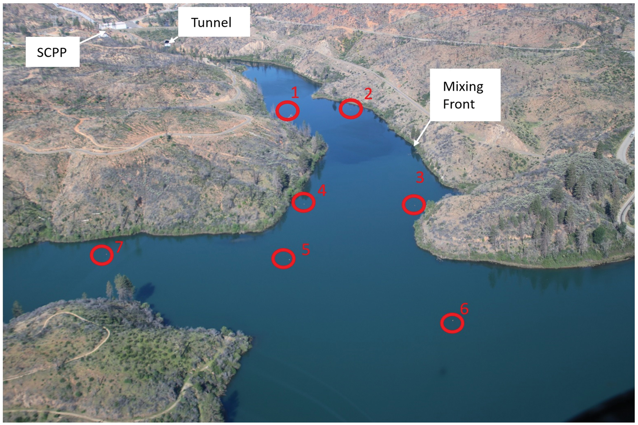
Water Quality Sondes
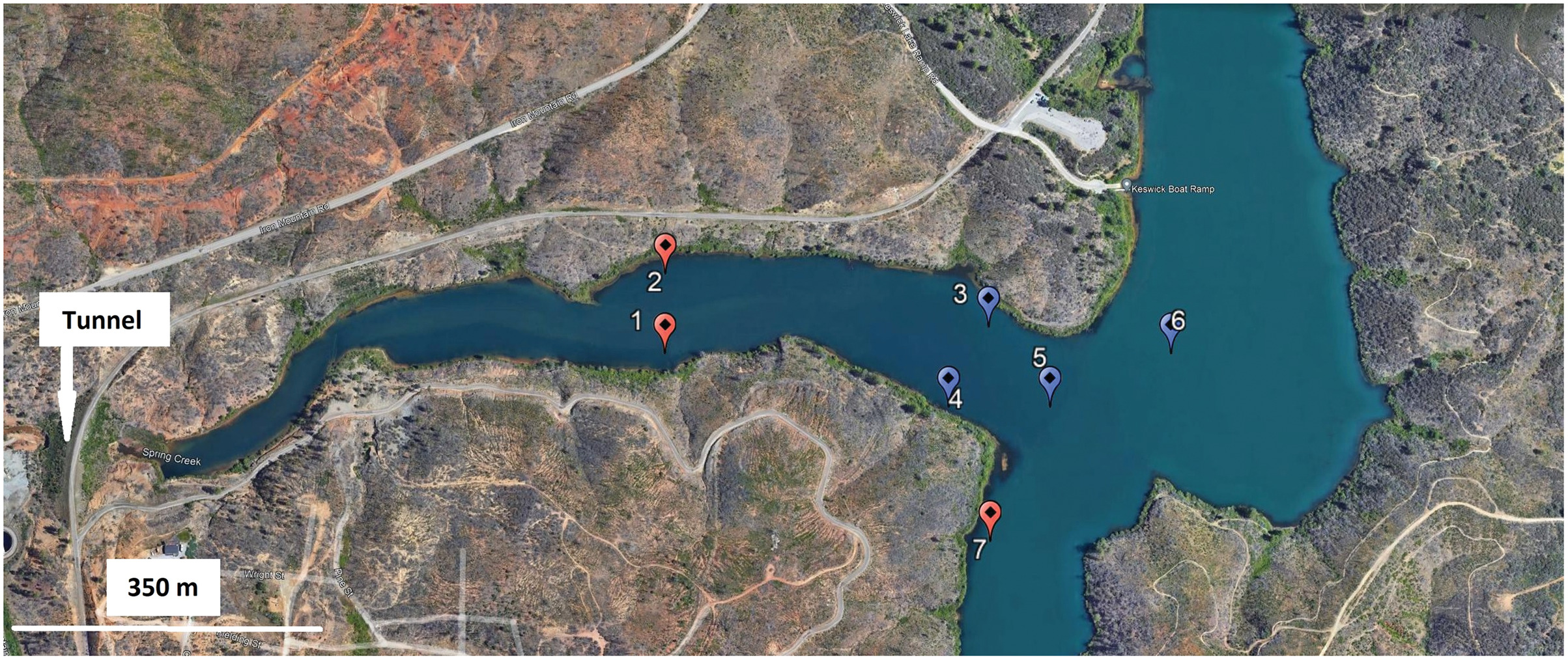
Ten water quality sondes were deployed at seven stations in and near the Spring Creek Arm (Fig. 4). Each station featured a steel anchor, mooring line, and surface float, with a sonde tied off near the reservoir bed. At Stations 1, 2, and 7, a second sonde was installed as close to the water surface as practical. Water depths at the seven stations ranged from 4.6 to 18.3 m at the time of installation. The water level rose and fell by approximately 1.5 m during the course of each day of the field study. The installation was designed so that the near-surface sondes would move with the water level, and the near-bed sensors would move only slightly. Seven Turner Designs Cyclops-7 sondes (San Jose, California) and three YSI EXO fluorometers (Yellow Springs, Ohio) were used. Each sonde reported the Rhodamine WT concentration and water temperature. The YSI sondes also reported pressure head and specific conductance (SpC). Each sonde was programmed to record data every 5 min. All sondes were installed several hours prior to the dye being released, and were recovered 4 days later.
Calibration of the Rhodamine WT sensors was checked in the office prior to installation, and again after use, using three standards created by serial dilution of the source dye. Pre- and postdeployment calibration slopes, relating reported concentration to known concentration, typically agreed within 10%. The mean of the pre- and postdeployment slopes was used to correct the reported data for use. Both manufacturers claim very low detection limits ( for the YSI sensors, and for the Turner Designs instrument), but based on laboratory testing that included overnight observations, is a more reasonable detection limit for both sensors in practice. YSI claims accuracy for their Rhodamine WT sensor. Turner Designs does not provide an estimated uncertainty.
Drifter Data
It was desired to collect data describing surface water pathlines and flow speeds within the reservoir during the experiment. Preliminary model runs indicated that surface flow speeds during the experiment would be . Speeds this low are difficult to measure in the field with anything other than fixed instrumentation, which in turn provide data for only a very limited number of locations. Surface drifters were designed and deployed to acquire flow pathline data that could be differentiated to compute Lagrangian speed data.
The drifters were constructed of PVC pipe and polyethylene tarp material, with closed-cell foam swimming pool noodles for buoyancy, following a design like that used by Lockridge et al. (2016) (Fig. 5). The sails of the drifters, each , were designed so that the product of the drag coefficient and the projected area for the underwater portion exceeded that of the subaerial portion by more than a factor of 40, as recommended by Niiler and Paduan (1995) to keep drifter motions attributable to wind acting on subaerial portions of the drifter below 1% of wind speed. The mean wind speed at the nearest airport (Redding, California) averaged for the first day of the experiment described here, and decreased thereafter. The reservoir water surface is sheltered, lying within a narrow, steep-walled canyon.
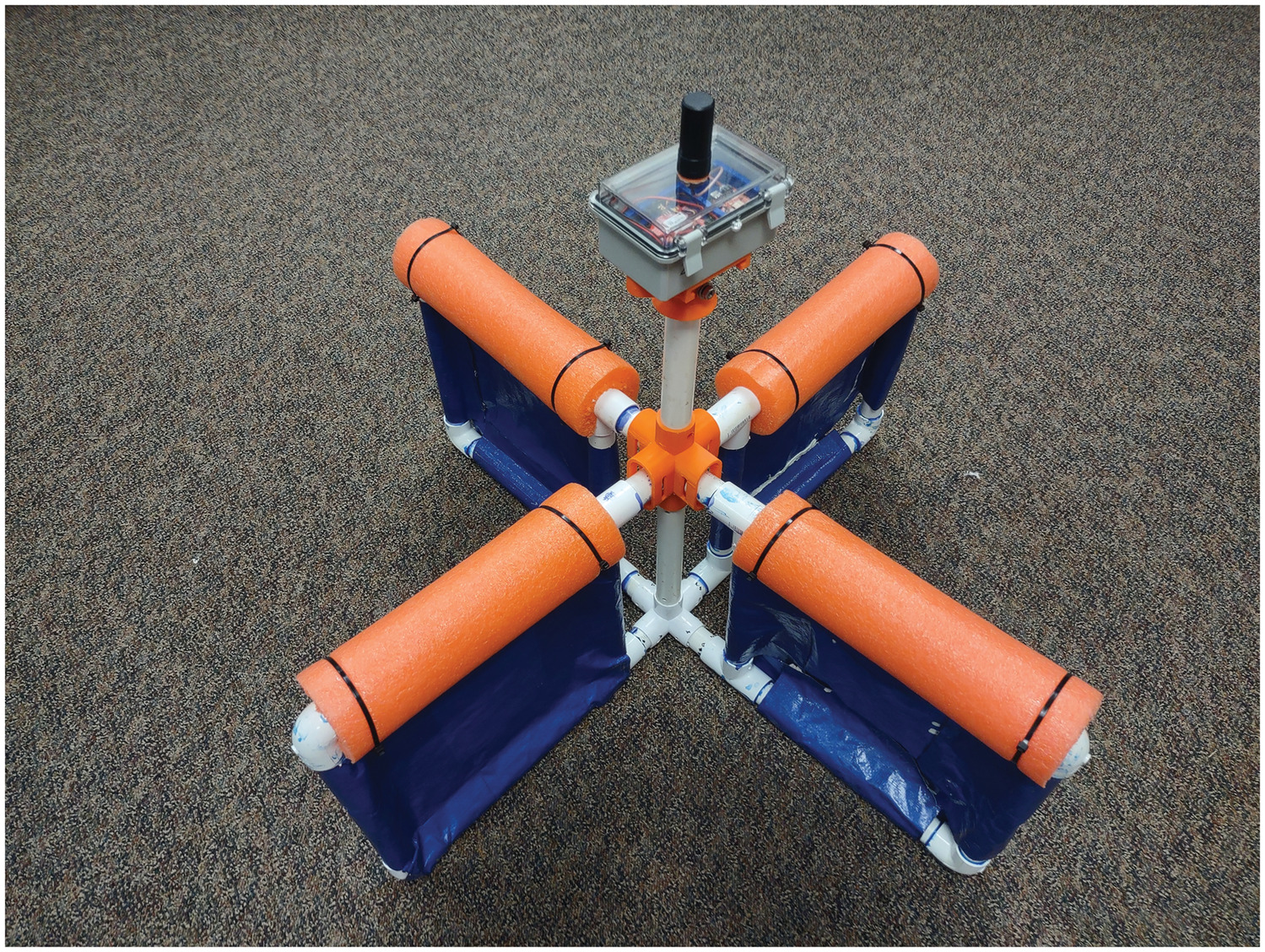
A short PVC mast held a small electronics box above the water surface (Fig. 5). Inside was a Sparkfun ZED-F9P dual-frequency GNSS receiver (Sparkfun, Boulder, Colorado), a Sparkfun Openlog Artemis data logger, a 1 Gb microSD card, and a rechargeable 3,200 mAh Li-Ion battery. A Sparkfun BT-560 GNSS multiband antenna was mounted to a bulkhead connector that passed through the lid of the box. The battery was sufficient to power the unit for 24 h with the GNSS receiver running constantly and the data logger sampling at 1 Hz. The manufacturer of the GNSS chip (uBlox, Zurich, Switzerland) claims centimeter-level accuracy with differential corrections of the GNSS observations. The total cost was less than $500/drifter.
For the Keswick Reservoir experiment, GNSS data from the mobile receivers were postprocessed using RTKLIB v2.4.2 software and data from the nearest National Oceanic and Atmospheric Administration (NOAA) Continuously Operating Reference Stations (CORS) network. Postprocessing of 8 h of data from a stationary base station deployed during the experiment revealed RMS position errors of 2 mm in both horizontal directions. Postprocessing the same data in kinematic mode revealed RMS position errors of less than 1 cm.
Three drifters were released shortly before the dye release into the Spring Creek Arm began. All three drifters went aground within 12 h of deployment, but the resulting reported pathlines (Fig. 6) revealed flow details not resolved in the numerical model, as discussed subsequently.
Modeling Guidance Derived from Analytical Solutions for Mixing
No analytical solutions are available to describe time-dependent mixing in a channel with arbitrary bathymetry, but a review of the available steady-state analytical solutions and relevant dimensionless parameters governing mixing in surface waters can define some expectations for the field site. Fischer et al. (1979) presented an equation for a constantly flowing effluent entering a channel with uniform cross section and constant flowrate. They recommend a transverse mixing coefficient ofwhere = water depth; and = shear velocity. Fischer et al. (1979) also recommend a vertical mixing coefficient one order of magnitude less than the transverse mixing coefficient. The mixing coefficients have dimensions of length squared per unit time, meaning that the time required for mixing throughout a given length is proportional to the square of that length. For a channel with a depth 1 order of magnitude less than its width (as in the Spring Creek Arm), the time required for mixing throughout the vertical dimension would be 2 orders of magnitude less than that required for mixing throughout the lateral dimension. For practical purposes, this means that mixing throughout the vertical dimension happens instantaneously.
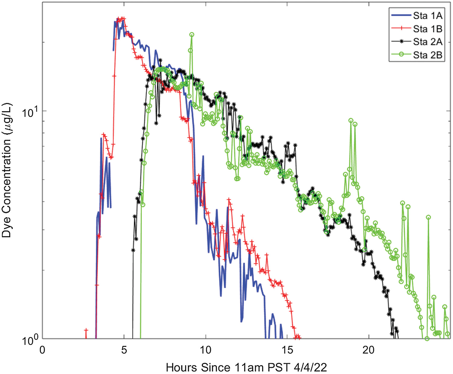
(1)
The corresponding distance downstream to the point at which mixing is complete across the channel cross section iswhere = mean flow speed in cross section; and = channel width (Fischer et al. 1979). For the Spring Creek Arm scenario, with shear velocity , transverse mixing coefficient , depth 3.5 m (range 1–15 m), and width 100 m (range 50–150 m), the resulting distance to full mixing is in the range 10–100 m for the flowrates typically encountered (). In the field the distance to full mixing will be influenced by bathymetry, roughness, flow temperatures, and so forth, but this result indicates that the flow should be fully mixed long before it reaches the end of the 1 km Spring Creek Arm, given sufficient time to reach steady state conditions. Field results were consistent with these estimates. The dye was fully mixed throughout the vertical at both Stations 1 and 2 for the first 5–12 h after dye arrival (Fig. 7). When concentrations dropped below about 20% of peak values, concentrations in the upper part of the water column dropped more quickly than at the bed. Cross-channel (horizontal) uniformity was reached several hours after the dye first reached Station 1. Station 2 is in the hydrodynamic shadow of a headland (Fig. 4), resulting in more-complicated flow that delayed the arrival of the dye compared with that at Station 1. The drifter tracks (Fig. 6) showed that the surface flow had a more direct path to the south bank of the channel, where Station 1 was located, than to the north bank location of Station 2.
(2)
The Richardson number represents the ratio of buoyancy forcing to the shearing forces that tend to enhance mixing
(3)
A Richardson number of 1 represents the scenario in which buoyancy and shear have similar degrees of competing influence on stratification. For the Spring Creek Arm scenario, with the discharge chosen to match the 2022 field experiment, a temperature difference of 0.8°C between the top and bottom layers of the flow was required to reach this condition (UNESCO 1981). It is not uncommon for the sources entering the Spring Creek Arm to have temperatures differing by more than this amount.
Modeling of Field Experiment Conditions
The Delft3D FM model was chosen to simulate flows and mixing in Keswick Reservoir (Deltares 2021a, b). This is a flexible mesh model with the capability to specify a stretched vertical coordinate system, solving unsteady shallow water equations with a choice of different turbulence models, during baroclinic or barotropic flow conditions.
Model Grid Scope and Resolution
An empirical equation for development length in open channels was used to optimize the size of the computational domain for modeling purposes, noting that only the downstream of Keswick Reservoir was of significant interest in the study. Wilkerson et al. (2019) developed an expression for the distance required for open channel flow to become uniformwhere = channel roughness. With roughness chosen conservatively as 0.002 m to represent sand, a mean depth of 10 m, and a channel width of 100 m, the distance to uniform flow is 1.3 km. One modeling grid that spanned all of Keswick Reservoir was developed, and a second that spanned the downstream third of the reservoir, reaching 1.3 km upstream of Flat Creek on the reservoir’s west bank (Fig. 1 shows the spatial extent). Comparing steady-state results across the reservoir near Flat Creek revealed differences of no more than in depth-averaged velocity. The smaller grid was deemed to be sufficiently large in extent, and was used for all subsequent model runs. Cell horizontal dimensions ranged from 2.5 to 10 m, with 10 computational layers each representing 10% of the water column. Bathymetric data were interpolated to establish a bottom elevation for each computational cell.
(4)
Boundary and Initial Conditions
Keswick Reservoir is heavily controlled and monitored. During the period of the 5-day field experiment, more than 90% of the water entering the reservoir was measured as it passed through a Reclamation-controlled facility. Hourly time-series data were obtained from Reclamation that described discharge, water level, and water temperature at boundary points of interest, and total inflow, computed from the water budget. The author measured the temperature of water exiting SCDD independently throughout the dye delivery period. This and other data from the field experiment were presented by Work (2022).
Depending on flow conditions, the travel time from Shasta Dam to the chosen upstream end of the model domain could be multiple days, and the water temperature can change as the flow travels downstream. Although temperature is not a conserved quantity, it was treated as such to compute a temperature time series at the upstream end of the model domain, using a mass balance approach and water temperature data measured near Shasta Dam. The result indicated that on average for the period simulated (March 28–April 15, 2022), water temperature increased by 0.9°C as flow traveled from Shasta Dam to the upstream end of the model domain. This correction was added to observed Shasta Dam outflow water temperatures to specify temperature at the upstream boundary of the model. Initial water temperature for the entire domain was set to match that observed at the upstream-most water-quality sonde deployed in the reservoir during the field experiment (10.3°C). Temperatures at the other sondes ranged from 9.5°C to 11.1°C, and the coldest temperatures were observed upstream in the Spring Creek Arm. A model spin-up time of 8 days was employed, making small errors in the chosen initial temperature unimportant. Specification of the time-dependent temperatures of the inflows during the simulation was found to exert a second-order effect on the model results, using the simplest transport-only model for heat flux in Delft3D FM, which neglects heat exchange with the atmosphere. Model runs performed to simulate hypothetical future scenarios neglected heat transport.
A conservative tracer was specified, in the form of salt, entering the domain via the SCDD. Inflow dye concentrations in Spring Creek, computed as described previously, were divided by 100 and specified as a salinity time series ranging from 0.07 to 1.37 parts per thousand (ppt) for modeling. This allowed for modeling of dye concentrations without introducing enough salt to the domain to significantly influence buoyancy.
Fig. 8 shows discharge and water level time series for the period of the field experiment. Discharge at Keswick Dam was held relatively steady for the entire period. Discharge from SCDD typically is close to zero, except just before or during a storm event. For the experiment, it was held close to for 24 h and then stopped. Flow from SCPP was held close to for the same 24-h period, and then the entire system returned to normal operations, with Shasta Dam and SCPP flows adjusted to meet daily power demands.
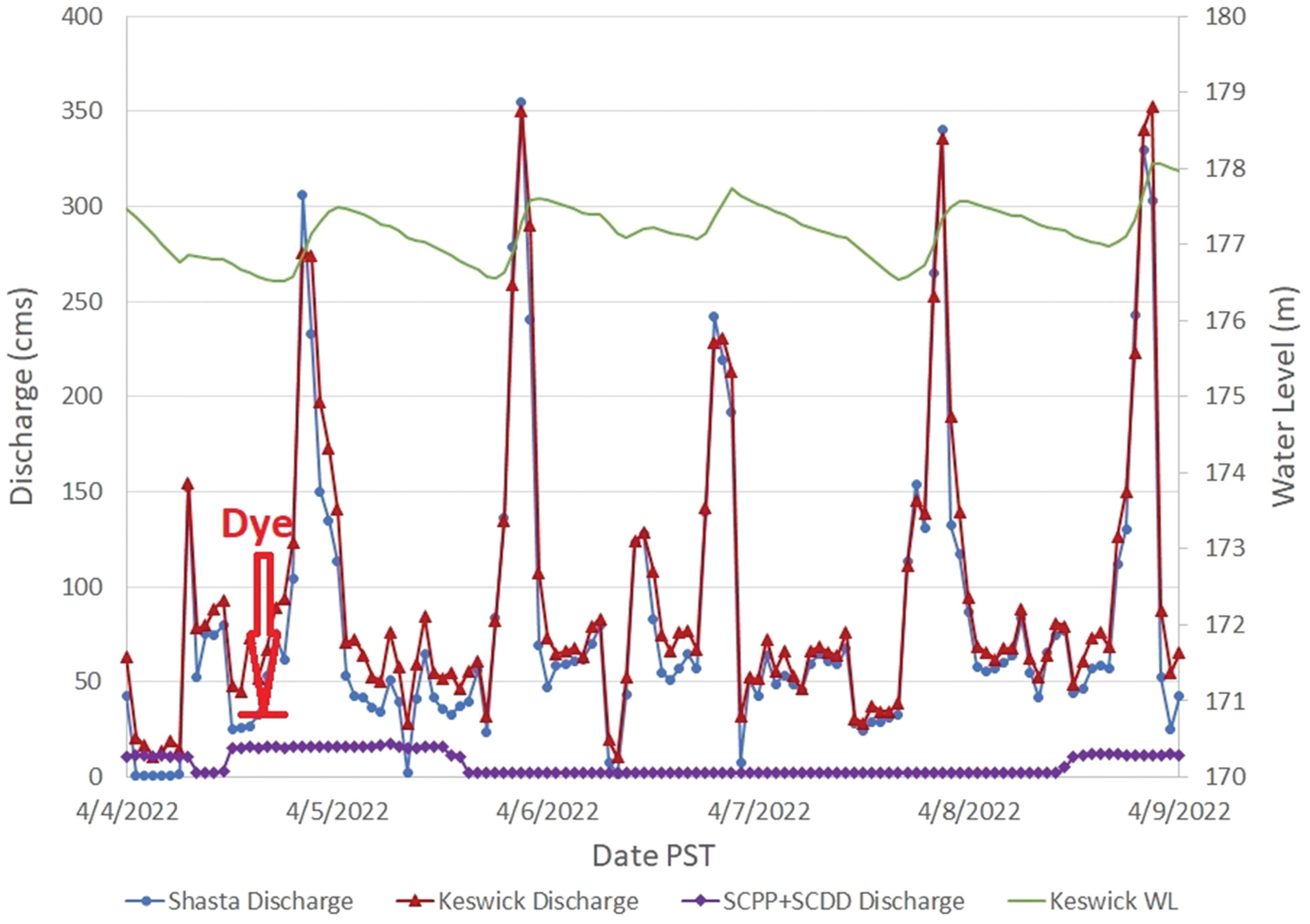
The temperature of the flow from SCDD increased by 0.9°C during the 24-h period of flow from this source. SCPP temperatures increased from 9.6°C to 10.4°C during the 12-day period modeled (March 28–April 8). Temperatures at Keswick and Shasta Dams were nearly constant during this period.
The starting water level for the model was specified based on values reported by Reclamation. The model computes subsequent water levels based on conservation of water mass.
Observed Dye Concentrations
The primary goal of the project was to reveal mixing patterns and their dependence on forcing, so dye hydrographs served as the primary metric for comparing model results to measurements. Dye was detected by all 10 deployed sondes, although the near-surface measurements at Station 7 were above the practical detection limit only momentarily, peaking at . Station 5 was located downstream of Station 4 but was also closer to the channel thalweg, and reached peak dye concentration earlier (Fig. 9). Full mixing across the cross section, observed at Stations 1 and 2 (Fig. 7), corresponded to at . Concentrations exceeding were measured at Stations 3, 4, and 5, indicating that the dye advanced all the way down the Spring Creek Arm before the cross section became mixed across the channel downstream at [Fig. 9(a)]. Some dye traveled upstream within the main body of the reservoir, near the bed, to Station 6. Concentration at Station 7B peaked at and stayed near or above half this value for the next three days [Fig. 9(b)].
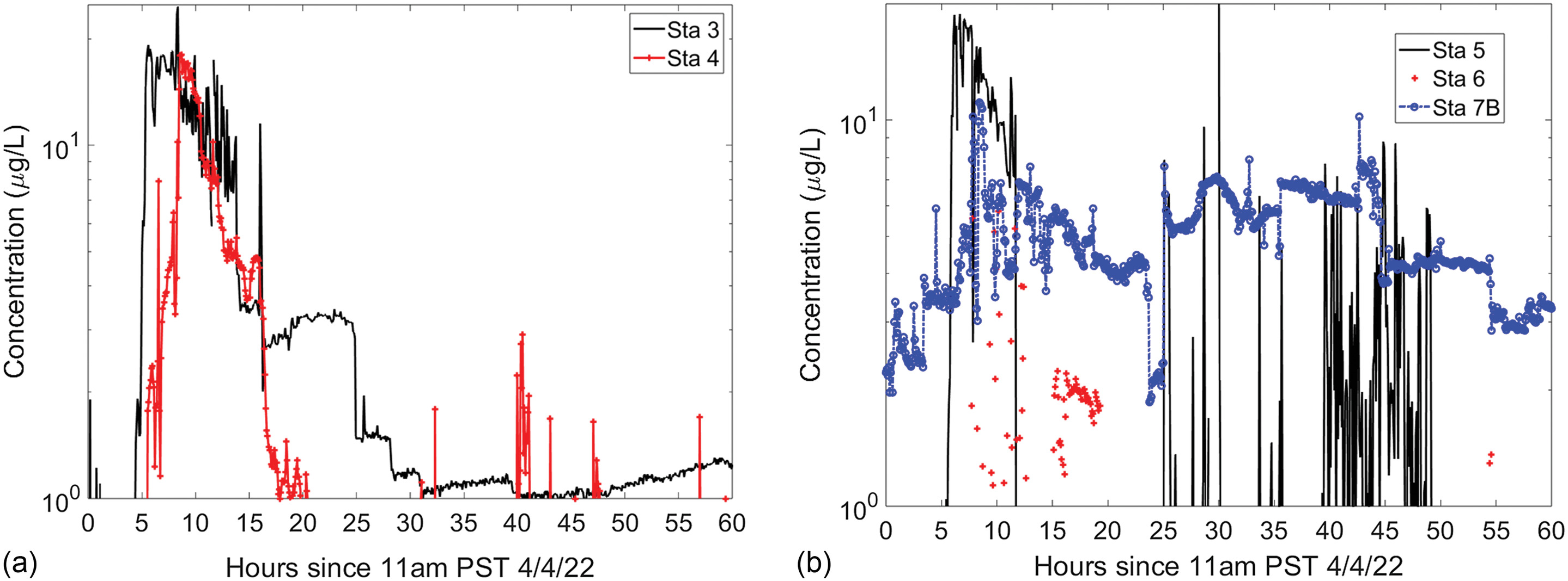
An aerial photo of the Spring Creek Arm taken the day following the dye introduction reveals a pattern seen in many of the numerical model results (Fig. 10). The waters arriving from Shasta Lake and SCPP have different colors. Shasta Lake water has pushed into the Spring Creek Arm, on the surface, and the flow from SCPP dives beneath to escape the Arm. This will deliver constituents traveling within the Arm into the lower layer of the main stem of the reservoir, consistent with the observations of dye concentration at Stations 7A and 7B.
The dye arrived as a sharp front at the three most upstream stations [Stations 1–2 (Fig. 7) and Station 3 (Fig. 9)], indicating a dominance of advection over diffusion. The time at which each of these stations first recorded was used as the metric for comparing model travel times to measurements. A RMS error was defined based on measured and modeled values of this time, considering all five sondes deployed at these three locations.
Model Sensitivity Tests
Model sensitivity tests considered the influence of bottom and sidewall friction coefficients and models, eddy viscosity model and coefficients, temperature model, inflow and outflow rates, inflow geometry, initial water level, wind, number of computational layers, and grid cell size. Many of these, such as wind, were found to have little influence on model results for the specific case considered. Inflows were modeled as depth-uniform flows distributed horizontally across one or more computational cells, and results were insensitive to slight changes in these definitions. This would not be true if near-field mixing were the focus, but in that case a different approach would be required, resolving vertical accelerations and using higher resolution.
The most influential input parameters were those controlling bottom friction and eddy viscosity, and resolution of the computational domain. In the end, 10 computational layers were used, with cell sizes nominally in the cross-flow and along-flow directions within the Spring Creek Arm, respectively. Higher resolution had little impact other than to increase run times. The temperature model used allowed for transport of heat only within the water, with no exchange with the overlying air. Turning this temperature model on resulted in second-order improvements to the results. With more extreme temperature differences between the different inflows, temperature would be more important to the model.
Numerical Energy Dissipation
Without any local data to justify an alternative definition, bottom friction and horizontal eddy viscosity were both treated as constants, in both space and time, during any given model run. The best model results were obtained when bottom friction and horizontal eddy viscosity were both set to extremely low values: 0.001 for Manning’s coefficient, and 0.005 for constant horizontal eddy viscosity (the -epsilon model was used to define variable vertical eddy viscosity). Both of these are an order of magnitude less than the default model values, prompting some investigation of energy dissipation within the numerical scheme of the model.
A seiche test was performed by defining a domain 1 km long by 100 m wide by 5 m deep, similar to the Spring Creek Arm, with 10 computational layers. An initial condition of a linearly sloping water surface along the length of the domain was specified—half of a sawtooth wave—along with closed boundaries on all sides. In the absence of friction and turbulent dissipation, with a perfect numerical scheme, the model should slosh forever. Initial amplitude was set to 0.05 m, Manning’s was set to zero, and horizontal and vertical eddy viscosity both were set to . The wave amplitude decayed to within 1% of its initial amplitude within 120 min, or 25 fundamental wave periods.
In the seiche test, for a unit width of channel the head (energy per unit weight) lost per unit length in the flow direction—the friction slope—is . A similar value was computed from results for the Spring Creek Arm best-fit case, with Manning’s set to 0.001. Although the two cases differ, this suggests that energy dissipation within the modeling scheme is the same order of magnitude as the energy loss being added by setting in the best-fit Keswick Reservoir simulation. The Manning equation was developed to describe uniform steady flows in open-channel scenarios (Chow 1959), but in a backwater condition such as that considered here, the friction slope is much less than the channel slope, so a much smaller value of is required to reproduce field observations. The results obtained here demonstrate that it would be difficult to simulate flows slower than with the model, using the Manning equation, because the energy dissipation implicit in the numerical scheme might then exceed actual field energy dissipation. At higher speeds, good results can be obtained with roughness values lower than might otherwise be expected, as was the case here.
Increasing the constant horizontal eddy viscosity had little impact on modeled arrival times of the dye cloud downstream, but led to more-rapid diffusion of the dye toward Station 2 than was observed. Small (10%–20%) changes in horizontal eddy viscosity away from the best-fit calibration value led to improvements at some measurement locations, but degradation of results at other sites.
Modeled Dye Hydrographs
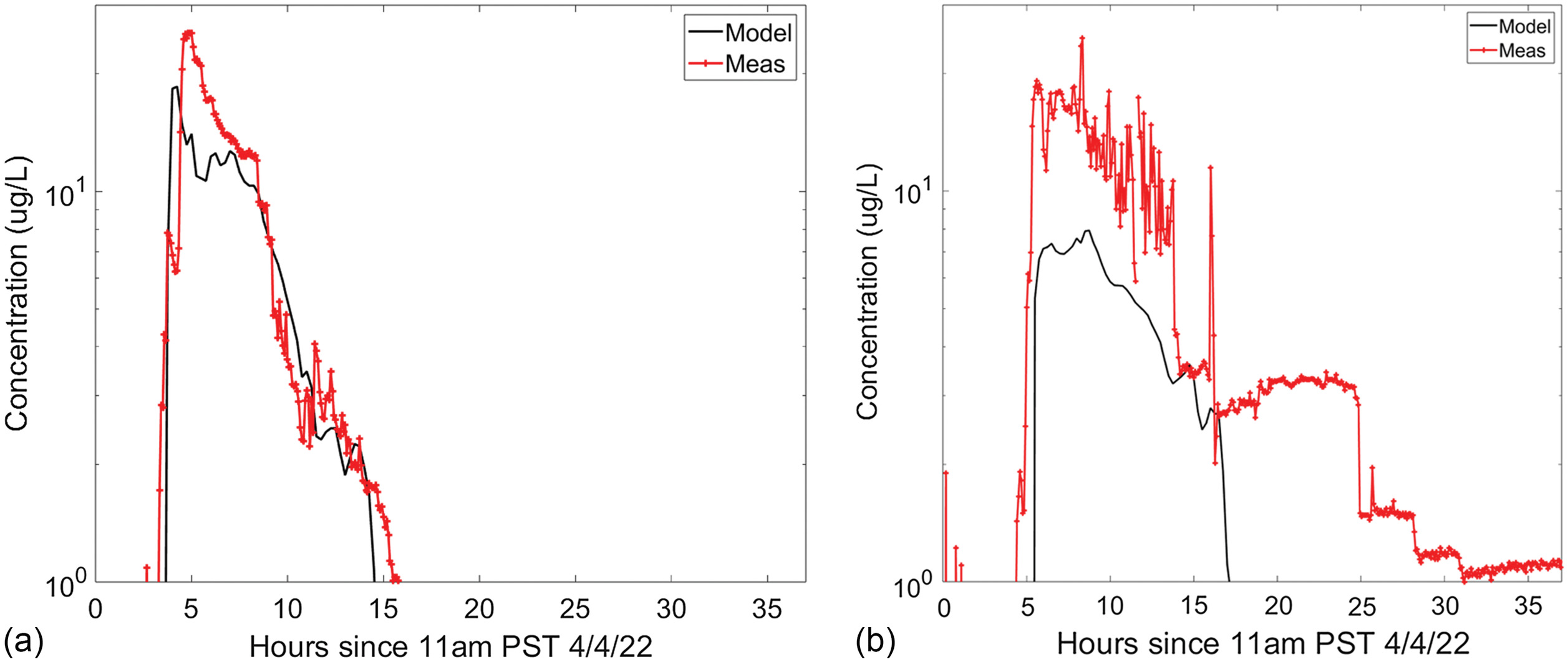
For the five sondes deployed at Stations 1–3 to measure both near-bed and near-surface dye concentrations, the RMS error in the arrival time of the dye (defined based on the first occurrence of ) was less than 6 min after model calibration. Fig. 11 shows the best and worst of these results for two near-bed sondes. In each case, the model closely matched the arrival time of the steep dye front, indicating that flow speeds were replicated accurately. The lack of vertical variation in concentration measured at Stations 1 and 2 in the field (Fig. 7) also was replicated, but the model underpredicted peak dye concentrations, indicating that the model may slightly underrepresent the rate of lateral mixing, given that the monitoring stations were located near the channel margins. Increasing horizontal eddy viscosity addressed this at some locations but negatively impacted estimates elsewhere. Advection and turbulence are the primary causes of the transport and mixing; the molecular diffusivity for salt in the model is treated as constant and is nearly 3 orders of magnitude less than the kinematic viscosity of the water.
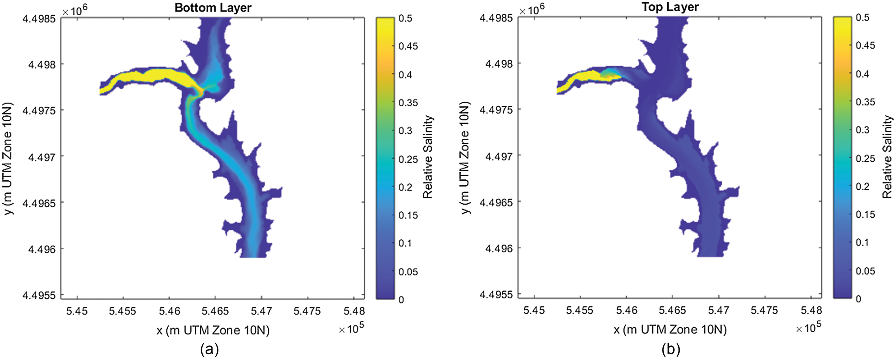
Results farther downstream were influenced by opposing surface flow entering the Spring Creek Arm from the main stem of Keswick Reservoir (Fig. 10). This was observed in nearly every model test, with and without temperature-induced stratification. Outbound flow from Spring Creek Arm, fully mixed throughout the vertical, dives below the incoming surface flow from the reservoir (Fig. 12). Some salt moves upstream on the bottom, and near-bottom salt gradually migrates vertically as it moves downstream. This result is consistent with the observation at Station 7 revealing near-bed concentrations much higher than near-surface values.
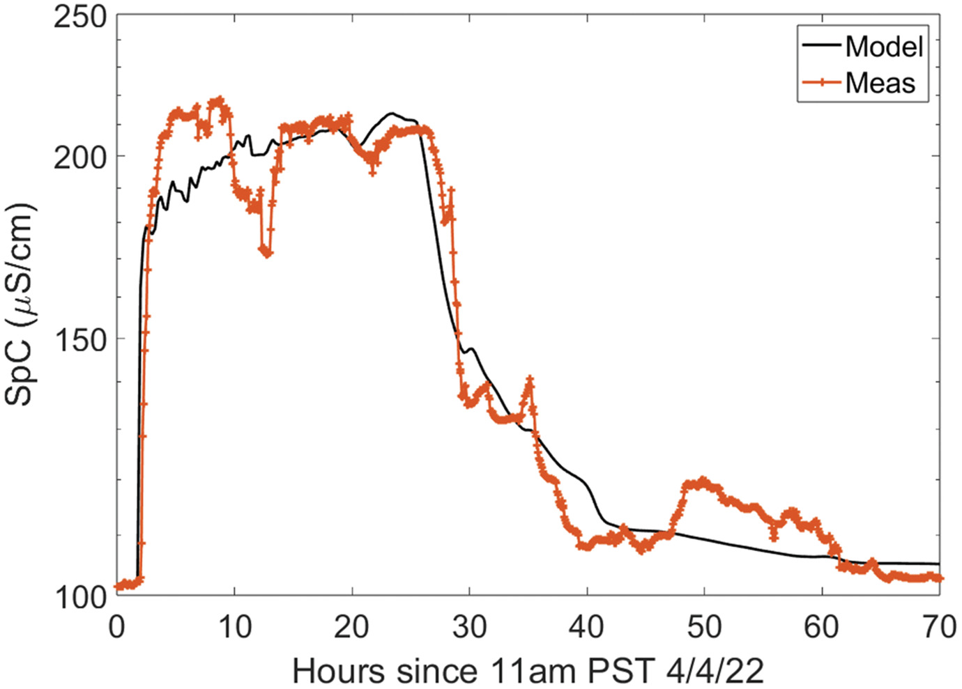
The calibrated model also was used to simulate specific conductance during the field experiment. Specific conductance of the outflow from SCDD was not measured, but the sonde at Station 1B reported a mean value of prior to the outflow from SCDD, and this increased to a mean of when the incoming flow passed by. Assuming full mixing of the cross section at this location, the specific conductance of the outflow from SCDD was estimated analytically to be , using a simple mass balance, and taken as a constant to define model input (the value measured 4 days later was ). The resulting time history from the model is shown in Fig. 13. This was not a true model validation test because it was the same case as the calibration tests, hydrodynamically, but it was a second test with a different tracer, and revealed that the hydrograph of the tracer again was a good match with what was measured at this location.
After calibration, the model was used to investigate steady-state results for 10 unique hypothetical cases (Work 2023). Increasing the flow from SCPP into the Spring Creek Arm results in nearly immediate dilution of the water being delivered by SCDD. Given sufficient time with constant inflows, the flow becomes fully mixed upstream of Stations 1 and 2, and an analytical estimate of steady-state dye concentration at these stations closely matched the model results. Fig. 14 shows dilution, defined as inflow concentration divided by local concentration, as estimated by the analytical model and the numerical model. Assuming zero concentration in the SCPP inflow, the analytical estimate of steady-state concentration at the midpoint of the Spring Creek Arm is simplywhere = concentration; and = water discharge. To estimate mean cross-sectional concentration at Keswick Dam, Eq. (5) was modified by adding Shasta Dam discharge, which also was assumed to be tracer-free, to the denominator.
(5)
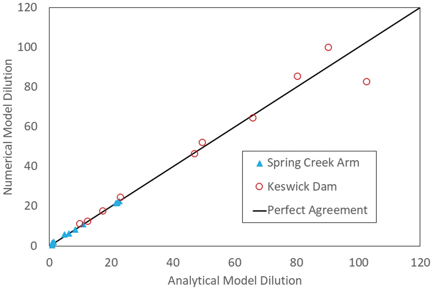
At the downstream end of the Spring Creek Arm, the high-concentration flow is confined to the bottom region of the channel, and cleaner water above, that has entered from the main stem of the reservoir, reduces the cross-sectional average concentration. Outgoing flow at the end of the Spring Creek Arm dives beneath the opposing incoming surface flow (Fig. 12), reducing the cross-sectional average concentration with little impact on the maximum value. The analytical modeling approach assumes both steady-state conditions and full mixing throughout the cross section, so this approach does not work well where large bathymetric gradients exist or intersecting flows meet. One might expect even better agreement than is shown in Fig. 14, but concentration is not a conserved quantity, and even though both models satisfy conservation of both water and constituent mass, they yield slightly different results when numerically modeled concentrations along a cross section are nonuniform.
The numerical model is orders of magnitude more complex than the analytical model in this case, but is required when forcing is time-dependent or when conditions prior to steady state are of interest. For even a small reservoir, this most often will be the case. For the 10 cases simulated to create Fig. 14, the time to reach steady state in the near-bed concentration computed at Keswick Dam ranged from 1.5 to 13 days. Even absent any rainfall within the watershed, it is unlikely that forcing would be held constant for multiple days (Fig. 8).
A simple estimate of the advection time scale for flow to travel from SCDD to Keswick Dam is a useful first-order estimator of the time required to reach steady-state concentration near the bed at Keswick Dam. The travel time was estimated aswhere and = length and mean flow speed in a reach of the channel, respectively; and subscripts 1 and 2 denote the Spring Creek Arm and the reach from its mouth to Keswick Dam, respectively. Modeled time to steady state was determined based on inspection of model results with 6–12 h resolution. The best-fit linear relation between the observed time to steady-state mixing and the analytical estimate of advection time scale [Eq. (6)] was , with and sample size . This result should be taken only as a first estimate, because it resulted in nearly a 50% error in one of the 10 cases.
(6)
Drifter Velocities
The model calibration focused on matching measured and modeled concentration time series. To get both the dye arrival time and its time history correct, the model must adequately represent both the hydrodynamics and the mixing processes in the model. The drifter position data, with O(1 cm) resolution, was not used for model calibration, but can reveal details of the flow field that are not evident in the numerical model, with resolution O(1–10 m). The drifter data also can serve as a check on computed surface velocities, recognizing that the model employed provides Eulerian velocities, compared with the Lagrangian approach inherent in drifter use.
The version of Delft3D FM used for this project (v2022.04) does not feature a functional particle-tracking algorithm, so the reported drifter positions were differentiated to compute flow speeds for comparison with model results. Drifter draft was similar to computational layer vertical thickness within the Spring Creek Arm. Model cell sizes in this region typically were long in the direction of flow, whereas with the GNSS receivers onboard the drifters sampling at 1 Hz while traveling at , drifter velocity data were available with 1–10 cm spatial resolution. Several postprocessing steps were required to facilitate comparison.
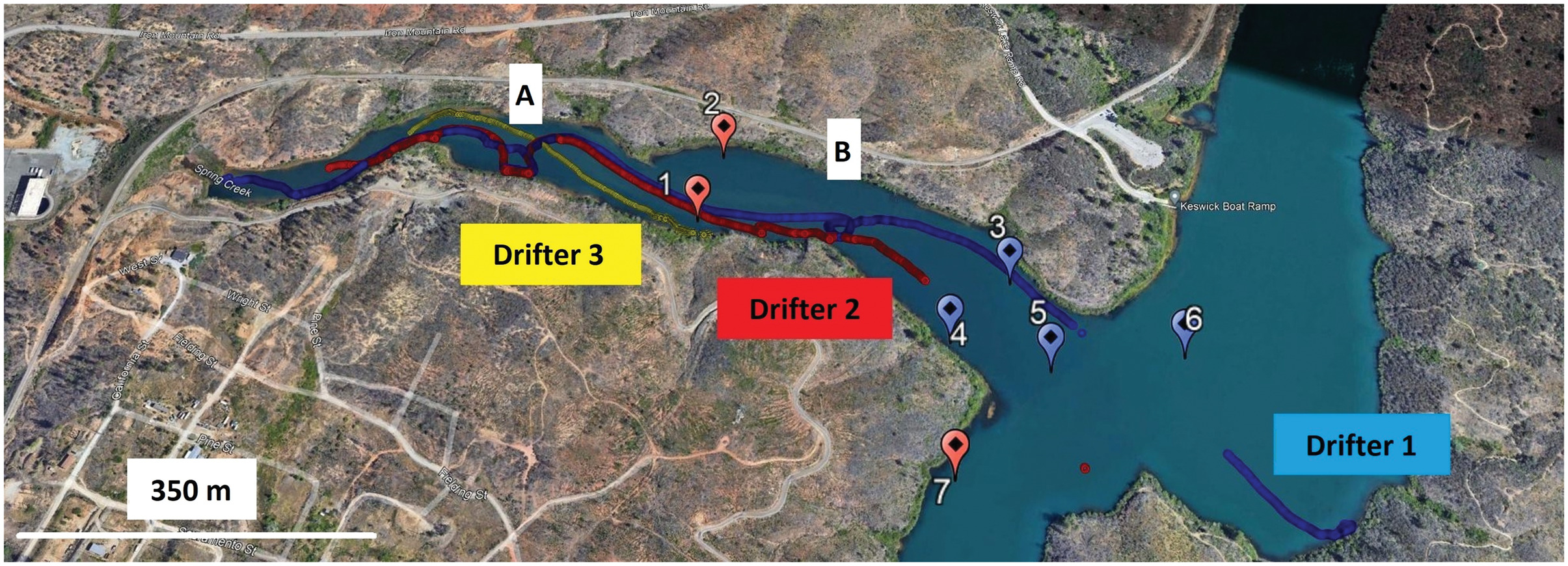
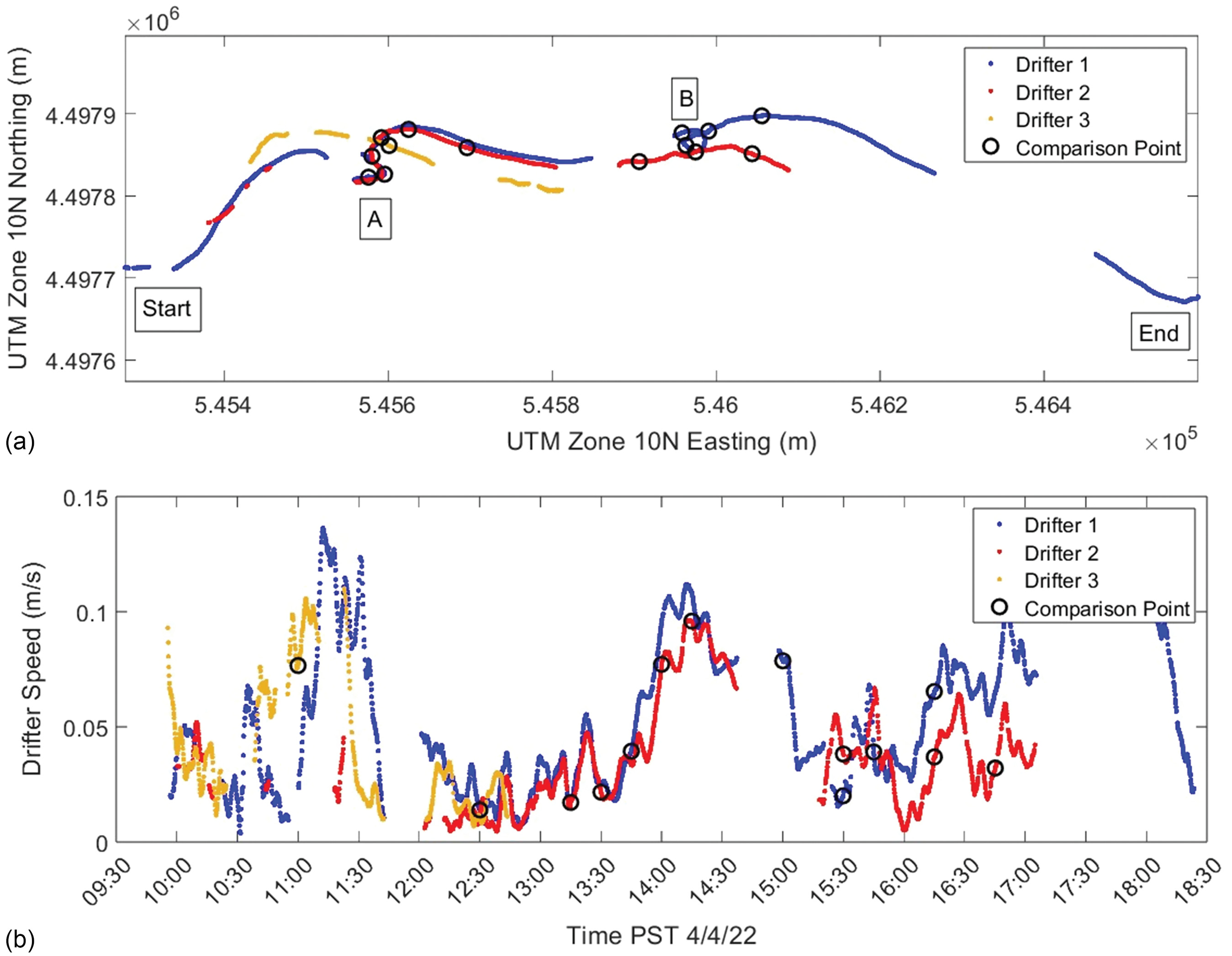
GNSS fixes based on float solutions were rejected in favor of fix solutions with integer ambiguity resolved, as were those with standard deviation of position in either north or east directions exceeding 3 cm. A 2.5-min moving average window was applied to the drifter velocity data to perform averaging over a spatial scale similar to the model resolution. The resulting drifter position and speed data are shown in Fig. 15. Drifters 1 and 2 followed similar paths, and both briefly were trapped in an eddy behind a small headland (Point A in Figs. 6 and 15), where they likely interacted with the channel bed. They both slowed as they approached the interface where incoming and outgoing flows met along the water surface in the Spring Creek Arm (Point B in Figs. 6 and 15; Fig. 10), and Drifter 1 followed a circular path there. Despite the inbound surface flow at the downstream end of the Spring Creek Arm predicted by the model, which was consistent with visual observations, Drifters 1 and 2 exited the Spring Creek Arm near the north and south banks, respectively (Fig. 6), and traveled across the main stem of the reservoir before going aground. Their paths across the reservoir would not be obvious based only on inspection of model surface velocity snapshots; this reveals the utility of a combined Eulerian–Lagrangian investigation (e.g., Pearson et al. 2021).
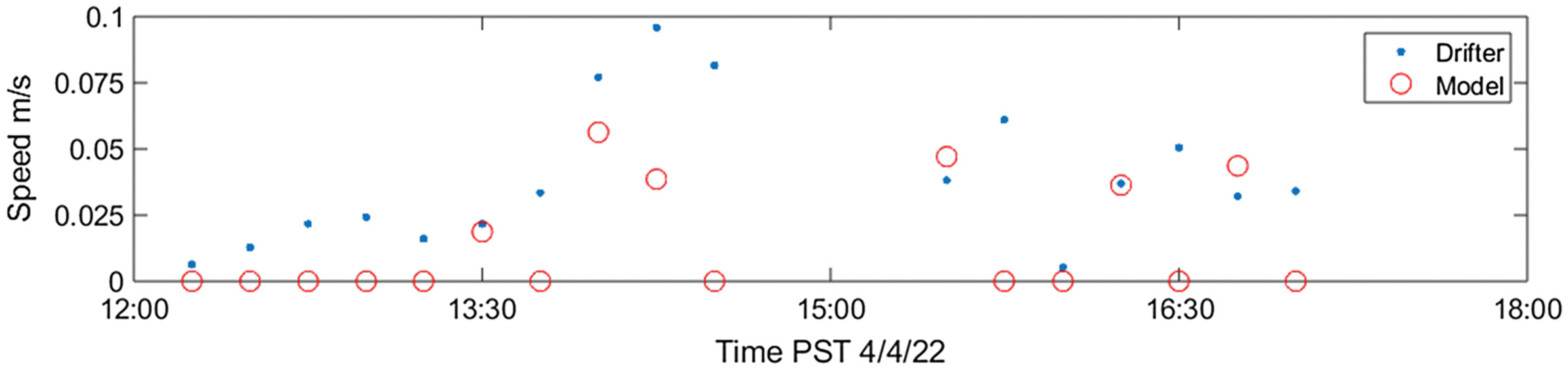
A comparison of drifter and model velocity magnitudes after matching them in time and space indicates limitations associated with the bathymetric survey data used in the study. The drifters often were near the southern boundary of the Spring Creek Arm (Fig. 6), in a region where computed flow speed is zero because model water depth is zero. Each of the three bathymetric surveys used in the study were performed by boat and did not resolve the shallowest regions along the edges of the Spring Creek Arm. Fig. 16 shows the results for Drifter 2; most computed flow speeds were zero at the positions reported by the drifter at the model output time of interest. Considering all three drifters, excluding times when computed flow speed was zero, the mean () drifter-derived speeds ware on average faster than the modeled speeds (mean drifter ). Some of this difference could be due to bathymetric survey or water level errors; recall the uncertainty in the vertical datum for both. A 15% error in cross-sectional area would be required to explain this speed difference, and the adjustments applied to the 2016 and 2021 surveys to force them to match with the 2010 survey were almost this large. Median values of computed standard deviations of the 1 Hz GNSS-derived positions were 1.2 and 0.9 cm for north and east directions, respectively. Assuming that these are representative of random, uncorrelated errors, a 2.5-min moving average (150 points) should reduce uncertainty in speed to less than . The differences between the modeled and measured flow speeds were near the measurement limit, and are concluded to be due to a combination of bathymetric survey accuracy and representativeness, water level error, GNSS position errors, and model error.
The drifter tracks reveal the integrated effect of the time-dependent flow on surface particle paths, and can reveal features that are not resolved within the model grid. Direct comparison of modeled and measured pathlines is preferable in the case of the low flow speeds such as encountered in this study, but the drifter-derived velocities provide validation that was not possible using only the dye hydrographs.
Summary and Conclusions
This study consisted of a short-term (days) field experiment focused on mixing processes in a long, narrow afterbay hydropower reservoir, and a numerical model of hydrodynamics and mixing in the downstream third of the reservoir. Details of the spatial and temporal evolution of the concentration field for a conserved tracer introduced to one arm of the reservoir were revealed. In this case, the reservoir is highly controlled and monitored, with four measured inflows and outflows typically accounting for more than 90% of the reservoir water budget.
The field experiment involved introducing 20% concentration Rhodamine WT fluorescent dye into one reservoir tributary during a 4.5-h period, resulting in concentrations near in the tributary, and leaving the reservoir. In between, dye concentrations were observed using 10 moored sondes at 7 locations. The flow delivering the dye was maintained at a nearly constant rate for 24 h, and the sondes remained in place for a total of 4 days.
The Delft3D FM numerical model was used to simulate reservoir hydrodynamics and mixing. Measured bathymetry, inflows and outflows, water temperature, and inflow concentration time series were used to drive the model, with modeled salinity serving as a proxy for Rhodamine WT dye concentration, both of which were assumed to be conserved. Observed concentration hydrographs served as the calibration target, with Manning’s (friction factor) and horizontal turbulent eddy viscosity, both of which were assumed to be constant within the domain, serving as calibration parameters.
Although this study focused on a specific reservoir, a similar strategy could be applied to investigate hydrodynamics and mixing at other sites. The results obtained here highlight the importance of having clearly defined flows of both water and constituents on all model boundaries, including definition of water temperatures so that the potential impacts of stratification can be considered. Model runs for this study made use of a vertically stretched coordinate system. The model also provides an option allowing for fixed thickness horizontal layers. The former option provides more realistic definition of bathymetry, whereas the latter may be preferable when stratification is strong. The drifter results reveal the importance of having accurate bathymetry data, particularly near wetting–drying boundaries that often are poorly resolved in bathymetric surveys.
Conclusions based on the Keswick Reservoir measurements and simulations are as follows:
1.
Analytical mixing solutions and dimensionless parameters representing the relative influence of different forcing mechanisms are useful both for study design and interpretation of results. In this study, a simple analytical estimate of steady-state concentrations closely matched three-dimensional (3D) numerical model estimates at selected locations. The numerical modeling approach is important to reveal details of flows within the reservoir, and for any results prior to steady state. Steady state is unlikely in this (and many other) reservoirs, with 1.5–13 days of constant forcing required for the cases simulated in this study.
2.
Sensitivity testing indicated that wind and water temperature were of negligible importance during the field study.
3.
Best-fit calibration required that both Manning’s and horizontal eddy viscosity be set to values an order of magnitude below the default model values. This was attributed to the low flow speeds [] encountered in the field study, resulting in little energy dissipation per unit distance traveled. A numerical seiche test indicated that energy dissipation within the numerical scheme is similar in magnitude to that introduced by the friction model in this low-speed scenario.
4.
Prediction of concentration at a specific point and time is challenging, especially within or downstream of regions with complicated hydrodynamics. The model used here worked well to identify the arrival time and duration of a contaminant pulse.
5.
Both analytical and numerical models indicated that complete cross-sectional mixing would be observed upstream of the upstream-most water quality sondes, consistent with field observations.
6.
The abundance of long-term data and existing bathymetric surveys for the site were of great benefit, providing information on frequency of occurrence and allowing for confident specification of forcing conditions.
7.
The high specific conductance of one water source relative to the receiving water allowed it to be used as an auxiliary tracer, in addition to the introduced Rhodamine WT dye. Although both tracers were transported by the same hydrodynamics, the similar quality results obtained with two different tracers delivered during different periods provides confidence in the transport modeling.
8.
Relatively inexpensive [ each (2021 costs)] surface drifters performed well; were easy to fabricate, deploy, and recover; and yielded higher resolution data and details of the flow field that were not readily evident in the model results. Their dual-frequency GNSS receivers, which were shown to provide O(1 mm) accuracy in static mode and O(1 cm) accuracy in kinematic mode, were critical in this case with low flow speeds. They also revealed limitations of the available bathymetric survey data.
Data Availability Statement
Acknowledgments
This study required the assistance of many individuals for the field study and associated logistics. The author particularly thanks David Hart (USGS), Selena Davila Olivera (University of Oregon, formerly USGS); Greg Gotham, Tyler Ward, Janet Martin, and Cary Fox (Bureau of Reclamation); Tom Wallis (Jacobs Engineering); Kate Burger, Stacy Gotham, and Bryan Smith (California State Water Resources Control Board); Charlie Alpers and Kate Campbell-Hay (USGS); and Lily Tavasolli (USEPA). The author also thanks Mike Deas and Ertugrul Sogutlugil from Watercourse Engineering for providing bathymetric survey data that were critical for the project. The project was supported by funding from the California State Water Quality Control Board (Grant No. 20-005-150), and by USGS Cooperative Matching Funds. Any use of trade, firm, or product names is for descriptive purposes only and does not imply endorsement by the US Government.
References
Alpers, C. N., H. E. Taylor, and J. L. Domagalski. 2000. “Metals transport in the Sacramento River, California, 1996-97.” Vol. 1 of Methods and data. Reston, VA: USGS.
Amorim, L. F., J. R. S. Martins, F. F. Nogueira, F. P. Silva, B. P. S. Duarte, A. A. B. Magalhaes, and B. Vincon-Leite. 2021. “Hydrodynamic and ecological 3D modeling in tropical lakes.” Appl. Sci. 3 (4): 444. https://doi.org/10.1007/s42452-021-04272-6.
Bencala, E., D. M. McKnight, and G. W. Zellweger. 1987. “Evaluation of natural tracers in an acidic and metal-rich stream.” Water Resour. Res. 23 (5): 827–836. https://doi.org/10.1029/WR023i005p00827.
Brenner, R., V. Magar, J. Ickes, E. Foote, J. Abbott, L. Bingler, and E. Crecelius. 2004. “Long-term recovery of PCB-contaminated surface sediments at the Sangamo-Weston/Twelvemile Creek/Lake Hartwell superfund site.” Environ. Sci. Technol. 38 (8): 2328–2337. https://doi.org/10.1021/es030650d.
Chen, S., J. C. Little, C. C. Carey, R. P. McClure, M. E. Lofton, and C. Lei. 2018. “Three-dimensional effects of artificial mixing in a shallow drinking-water reservoir.” Water Resour. Res. 54 (1): 425–441. https://doi.org/10.1002/2017WR021127.
Chow, V. T. 1959. Open-channel hydraulics. New York: McGraw-Hill.
Cole, T. M., and S. A. Wells. 2015. CE-QUAL-W2: A two-dimensional, laterally averaged, hydrodynamic and water quality model, Version 3.72. Portland, OR: Portland State Univ.
Cowie, R., M. Williams, M. Wireman, and R. Runkel. 2014. “Use of natural and applied tracers to guide targeted remediation efforts in an acid mine drainage system, Colorado Rockies, USA.” Water 6 (4): 745–777. https://doi.org/10.3390/w6040745.
Deas, M., and I. E. Sogutlugil. 2017. Keswick Reservoir bathymetric study. Davis, CA: Watercourse Engineering.
Deltares. 2021a. “D-flow flexible mesh.” In Computational cores and user interface. Delft, Netherlands: Deltares.
Deltares. 2021b. “D-flow flexible mesh.” In Technical reference manual. Delft, Netherlands: Deltares.
Fischer, H. B., E. J. List, R. C. Y. Koh, J. Imberger, and N. H. Brooks. 1979. Mixing in inland and coastal waters. Cambridge, MA: Academic Press.
Kilpatrick, F. A., and J. F. Wilson Jr. 1989. Measurement of time of travel in streams by dye tracing. Reston, VA: USGS.
Kimball, B. A., R. L. Runkel, K. Walton-Day, and K. E. Bencala. 2002. “Assessment of metal loads in watersheds affected by acid mine drainage by using tracer injection and synoptic sampling: Cement Creek, Colorado, USA.” Appl. Geochem. 17 (9): 1183–1207. https://doi.org/10.1016/S0883-2927(02)00017-3.
Lemly, A. D. 1997. “Ecosystem recovery following selenium contamination in a freshwater reservoir.” Ecotoxicol. Environ. Saf. 36 (3): 275–281. https://doi.org/10.1006/eesa.1996.1515.
Lockridge, G., B. Dzwonkowski, R. Nelson, and S. Powers. 2016. “Development of a low-cost Arduino-based sonde for coastal applications.” Sensors 16 (4): 528. https://doi.org/10.3390/s16040528.
Niiler, P. P., and J. D. Paduan. 1995. “Wind-driven motions in the Northeast Pacific as measured by Lagrangian drifters.” J. Phys. Oceanogr. 25 (11): 2819–2830. https://doi.org/10.1175/1520-0485(1995)025%3C2819:WDMITN%3E2.0.CO;2.
Nordstrom, D. K., and C. N. Alpers. 1999. “Negative pH, efflorescent mineralogy, and consequences for environmental restoration at the Iron Mountain Superfund Site, California.” Proc. Natl. Acad. Sci. 96 (7) 3455–3462. https://doi.org/10.1073/pnas.96.7.3455.
Nordstrom, D. K., C. N. Alpers, J. A. Coston, H. E. Taylor, R. B. McCleskey, J. W. Ball, S. Ogle, J. S. Cotsifas, and J. A. Davis. 1999. “Geochemistry, toxicity, and sorption properties of contaminated sediments and pore waters from two reservoirs receiving acid mine drainage.” In Proc., Technical Meeting, Hydrology Program, edited by D. W. Morganwalp and H. T. Buxton, 289–296. Reston, VA: USGS.
Nordstrom, D. K., J. M. Burchard, and C. N. Alpers. 1990. “The production and variability of acid mine drainage at Iron Mountain, California: A superfund site undergoing rehabilitation.” In Acid mine drainage-designing for closure, edited by J. W. Gadsy, J. W. Malick, and S. J. Day, 23–33. Vancouver, BC, Canada: BiTech.
Northern California Water Association. 2006. “Sacramento Valley integrated regional water management plan.” Accessed December 5, 2006. https://norcalwater.orgefficient-water-management/efficient-water-management-regional-sustainability/regional-planning/irwmp/.
Park, I., and I. W. Seo. 2018. “Modeling non-Fickian pollutant mixing in open channel flows using two-dimensional particle dispersion model.” Adv. Water Resour. 111 (Jan): 105–120. https://doi.org/10.1016/j.advwatres.2017.10.035.
Pearson, S. G., E. P. L. Elias, M. van Ormondt, F. E. Roelvink, P. M. Lambregts, Z. Wang, and B. van Prooijen. 2021. “Lagrangian sediment transport modelling as a tool for investigating coastal connectivity.” In Proc., Coastal Dynamics Conf. 2021. Delft, Netherlands: Delft Univ. of Technology.
Runkel, R. L., K. E. Bencala, B. A. Kimball, K. Walton-Day, and P. L. Verplanck. 2009. “A comparison of pre-and post-remediation water quality, Mineral Creek, Colorado.” Hydrol. Processes 23 (23): 3319–3333. https://doi.org/10.1002/hyp.7427.
Skjolding, L. M., L. V. G. Jørgensen, K. S. Dyhr, C. J. Köppl, U. S. McKnight, P. Bauer-Gottwein, P. Mayer, P. L. Bjerg, and A. Baun. 2021. “Assessing the aquatic toxicity and environmental safety of tracer compounds Rhodamine B and Rhodamine WT.” Water Res. 197 (Jun): 117109. https://doi.org/10.1016/j.watres.2021.117109.
Turunen, K., T. Räsänen, E. Hämäläinen, M. Hämäläinen, P. Pajula, and S. P. Nieminen. 2020. “Analysing contaminant mixing and dilution in river waters influenced by mine water discharges.” Water Air Soil Pollut. 231 (Jun): 317. https://doi.org/10.1007/s11270-020-04683-y.
UNESCO. 1981. The practical salinity scale 1978 and the international equation of state of seawater 1980. Paris: UNESCO.
Wilkerson, G., S. Sharma, and D. Sapkota. 2019. “Length for uniform flow development in a rough laboratory flume.” J. Hydraul. Eng. 145 (1): 06018018. https://doi.org/10.1061/(ASCE)HY.1943-7900.0001554.
Wilson, J. F. 1968. “Fluorometric procedures for dye tracing.” In Techniques of water-resources investigations, 31. Reston, VA: USGS.
Wilson, J. F., E. D. Cobb, and F. A. Kilpatrick. 1986. “Fluorometric procedures for dye tracing.” In Techniques of water resources investigations, 43. Reston, VA: USGS.
Work, P. A. 2022. Evaluation of hydrodynamic mixing in Keswick Reservoir, California, 2021-22. Reston, VA: USGS.
Work, P. A. 2023. Keswick Reservoir, California, Delft3D-FM model archive. Reston, VA: USGS.
Information & Authors
Information
Published In

Journal of Environmental Engineering
Volume 149 • Issue 10 • October 2023
Copyright
This work is made available under the terms of the Creative Commons Attribution 4.0 International license, https://creativecommons.org/licenses/by/4.0/.
History
Received: Dec 21, 2022
Accepted: Jun 19, 2023
Published online: Aug 10, 2023
Published in print: Oct 1, 2023
Discussion open until: Jan 10, 2024
ASCE Technical Topics:
- Chemical compounds
- Chemicals
- Chemistry
- Dyes
- Engineering fundamentals
- Environmental engineering
- Fluid dynamics
- Fluid mechanics
- Hydration
- Hydraulic engineering
- Hydraulic structures
- Hydrodynamics
- Hydrologic engineering
- Hydrologic models
- Hydrologic properties
- Hydrology
- Inflow
- Laminating
- Materials engineering
- Materials processing
- Models (by type)
- Numerical models
- Reservoirs
- River engineering
- Rivers and streams
- Water and water resources
- Water temperature
Authors
Metrics & Citations
Metrics
Citations
Download citation
If you have the appropriate software installed, you can download article citation data to the citation manager of your choice. Simply select your manager software from the list below and click Download.