Quantifying Mixing in Sewer Networks for Source Localization

Sonnenwald, Fred; Shuttleworth, Joe; Bailey, Olivia; Williams, Margaret; Frankland, James; Rhead, Becky; Mark, Ole; Wade, Matthew J.; Guymer, Ian

doi:10.1061/JOEEDU.EEENG-7134

Open access

Technical Papers

Mar 6, 2023

Quantifying Mixing in Sewer Networks for Source Localization

Authors: Fred Sonnenwald, Ph.D. https://orcid.org/0000-0002-2822-0406 [email protected], Joe Shuttleworth, Olivia Bailey, Ph.D. https://orcid.org/0000-0003-2812-9714, Margaret Williams, James Frankland, Becky Rhead, Ole Mark, Ph.D. https://orcid.org/0000-0002-7218-3606, Matthew J. Wade, Ph.D. https://orcid.org/0000-0001-9824-7121, and Ian Guymer, Ph.D. https://orcid.org/0000-0002-1425-5093Author Affiliations

Publication: Journal of Environmental Engineering

Volume 149, Issue 5

https://doi.org/10.1061/JOEEDU.EEENG-7134

PDF

Abstract

There has been a recent increase of interest in sewer network water quality, both for pollutants and wastewater epidemiology. Of particular interest is the ability to perform cost-effective small-scale monitoring to understand the sewer network and perform source localization (the process of identifying the sources of materials of interest within the network), enabling prioritization of combined sewer overflow (CSO) interventions and targeted response to the detection of infectious diseases. Rhodamine WT fluorescent dye tracing was carried out in the combined sewer networks of four UK cities, for which network geometries were available. Over 100 dye concentration profiles were recorded, from which discharge, travel time (velocity), and dispersion were quantified. A simplified hydraulic and water quality (conservative solute transport) modeling approach was used to investigate dispersion further. A theoretical method for calculating dispersion over a reach with nonuniform properties was derived and used with the models and recorded data to develop a method for estimating the dispersion coefficient in sewers. Novel simultaneous injections into multiple manholes within one sewer network were conducted. Modeling of these injections validated the modeling approach and explained the measured concentration profiles, demonstrating both the potential of hydraulic and solute transport modeling and the new dispersion coefficient predictor for source localization. Such modeling can be used to develop sewer network “fingerprints” and source location probability plots based on residence time distribution (RTD) theory to maximize information from limited water quality monitoring. This will aid managers and operators in identifying potential intermittent sources of material within the network.

Introduction

In the UK, over 400,000 combined sewer overflow (CSO) spill events were reported in 2020 (Environment Agency 2022). There has been significant public interest in storm overflows, and the Environment Act 2021 (UK Parliament 2021) obliges UK water companies to reduce storm overflows and their impacts. In the United States, the US EPA reports a $48 billion investment is needed for CSO correction, 18% of the total investment needed to meet federal water quality objectives (US EPA 2016). Similar issues exist worldwide (e.g., Botturi et al. 2021; Petrie 2021). Simultaneously, several recent studies have reported the presence of SARS-CoV-2 (COVID-19) within sewage (e.g., Mallapaty 2020; Medema et al. 2020) and the UK Government’s Environmental Monitoring for Health Protection (EMHP) program, led by the UK Health Security Agency, demonstrated government willingness to investigate the value of wastewater monitoring to track COVID-19 through sewer networks (UK Health Security Agency 2022). Both cases require an understanding of where the material has originated and its temporospatial variation throughout the sewer network. For CSOs this is to evaluate and prioritize interventions, and for public health monitoring to localize outbreaks. Thus, there is now a collective and significant interest in sewer network water quality and the information that can be obtained from wastewaters (Scassa et al. 2022). This interest is only expected to grow (Manuel et al. 2022).

The traditional and overarching priority for water companies is water quantity and ensuring sufficient network capacity to transport sewage to downstream treatment. For this, water companies typically use hydraulic sewer models such as InfoWorks ICM, MIKE URBAN+, or SWMM (Obropta and Kardos 2007), which are calibrated/validated using in situ flow monitoring (Titterington et al. 2017). In contrast to hydraulic models, where the key concern is how much water there is at any point in time, water quality models are more concerned with where that water originates from and what it contains. Although hydraulic sewer model software can evaluate water quality (e.g., Garsdal et al. 1995; Mark 2005), sewer models are rarely configured or calibrated to do so. When sewer network water quality models are used, they are calibrated for specific sections of interest (e.g., Magnusson et al. 1998; Balmforth et al. 2002), and in practice tend to perform poorly (Jia et al. 2021).

Many water quality models are physics-based (Jia et al. 2021) and rely on a description of solute transport, such as the advection-dispersion equation (ADE), utilized in conjunction with the hydraulic portion of a network model. In a 1-dimensional (1D) sewer network the ADE is

\frac{\partial c}{\partial t} + U \frac{\partial c}{\partial x} = D_{x} \frac{\partial^{2} c}{\partial x^{2}}

(1)

where

c

= concentration;

t

= time;

U

= mean longitudinal velocity;

x

= longitudinal position; and

D_{x}

= longitudinal dispersion coefficient (Fischer et al. 1979). While

U

is provided by the solved hydraulics, choice of

D_{x}

is problematic and poorly quantified in sewer networks. MIKE URBAN+ suggests a relationship between dispersion and velocity in the form of

D_{x} = a | U |^{b}

, where

a

and

b

are user-specified coefficients, typically taking values of 2 and 0 respectively, for a constant dispersion of

2 m^{2} / s

(Bouteligier et al. 2005; DHI A/S 2020; Zehnder 2021). InfoWorks ICM suggests

D_{x} = a u^{*} B

, where

a

is a user-specified constant with a default value of 0,

u^{*}

is shear velocity, and

B

is channel breadth, for dispersion of

0 m^{2} / s

, i.e., no dispersion (Innovyze Inc. 2022). Previous studies (e.g., Magnusson et al. 1998; Bouteligier et al. 2005; Rieckermann et al. 2005) have shown that neither is appropriate and dispersion must be correctly accounted for.

In normal dry weather flow conditions where sewer pipes act as channels, Rieckermann et al. (2005) found the magnitude of dispersion within sewers tended to vary little between networks, with most sewers having

D_{x} \approx 0.2 m^{2} / s

. Sokáč and Velísková (2016) report similar values. Dispersion in sewers in surcharged conditions may be an order of magnitude higher than in dry weather flow (Boxall et al. 2003) where hydraulic structures such as manholes contribute significantly to dispersion (Sonnenwald et al. 2021). Dispersion in sewers shows the expected scaling with velocity (Fischer et al. 1979; Rieckermann et al. 2005; Sokáč and Velísková 2021).

Rieckermann et al. (2005) identified several predictors for

D_{x}

in open-channel sewer flow, falling into two main categories: dispersion in irregular channels (e.g., Fischer 1975) and dispersion in a partially full pipe (e.g., Sooky 1969). The predictors identified were largely theoretical but modified by assumptions of flow conditions, typically containing terms for width, friction, velocity, and/or shear velocity (friction and shear velocity being difficult to obtain in practice). Although they found that the majority of predicted dispersion coefficients were within one order of magnitude of the measured value, Rieckermann et al. (2005) recommended new measurements when accuracy was required.

Fluorescent dye tracing has a wide variety of applications (Swarnkar et al. 2022), including model validation (e.g., Garsdal et al. 1995; Magnusson et al. 1998), and particularly is often used in determining

D_{x}

(e.g., Guymer and O’Brien 2000; Boxall et al. 2003; Istók and Kristóf 2014). Most fluorescent dyes are largely conservative, have low limits of detection, and can be continuously monitored (Wilson et al. 1984). To determine

D_{x}

, the fluorescent dye is injected at an upstream location, concentrations are monitored at one or more downstream locations that may be up to tens of kilometers apart, and

D_{x}

is calculated from the increase in the variance of the concentration distributions, or other methods such as optimization (Fischer et al. 1979; Guymer and O’Brien 2000). Fluorescent dye can be used to determine discharge by assuming conservation of mass (Fischer et al. 1979; Turner Designs Inc. 2022b) and to calibrate flow meters (e.g., Stonehouse et al. 2001; Lepot et al. 2014). Dye tracing in sewer networks can be simultaneously used to generate model validation data, confirm network geometry, estimate discharge, and determine the dispersion coefficient.

Source localization is the concept of identifying the sources of materials (chemicals, viruses, pollutants, etc.) monitored at a downstream location. The ideal approach, although prohibitively expensive, would be the placement of sensors at every manhole in a sewer network. Several studies (e.g., Wei et al. 2019; Bartos and Kerkez 2021; Chachuła et al. 2022) have investigated how to intelligently place as few as possible sensors within a network (be it a sewer, river, or water distribution network) for maximum coverage using computational methods. For complete network coverage and localization, the studies report that on the order of 30%–50% of nodes must be monitored, and there is a clear link between increased sensor data and increased prediction accuracy (Adedoja et al. 2018). In practice, there is some consideration to be made of the costs of extensive sensor networks, and the health and safety issues associated with the installation and maintenance of these sensors, particularly in sewer networks. Intending to rapidly identify a source of virus within a sewer network, Nourinejad et al. (2021) present a hybrid sensor and manual sampling approach to optimally place a small number of sensors (a few percent) that minimizes the need for manual sampling.

There is a clear reliance of source localization on water quality and, hence, solute transport modeling. Piazza et al. (2022) found that correctly accounting for dispersion significantly affected optimal sensor placement. Bartos and Kerkez (2021) demonstrate this link explicitly, using a finite difference solution to Eq. (1) in their work. Both Grbčić et al. (2021) and Zehnder (2021) used hydraulic and solute transport model outputs to train machine learning models to identify pollutant sources. These approaches tackle the challenges of unknown injection volume, type, and duration, but require output from accurate modeling of the system/flows. These studies highlight the importance of understanding the spread (dispersion) of material, but despite the reliance of source localization on solute transport modeling, most studies give little consideration to the choice of dispersion coefficient. Further, there is a need for data to validate sewer network water quality models (Jia et al. 2021). The aims and objectives of this paper are therefore to:

•

collect and analyze fluorescent dye traces in sewer networks and interpret this data to determine discharge, travel time (velocity), and dispersion coefficient;

•

compare these results against predictors of dispersion coefficient, providing a recommendation for predicting dispersion coefficient in sewers; and

•

employ solute transport modeling of the traced sewer networks to investigate source localization and suggest what information may be obtainable with limited monitoring.

Field Work

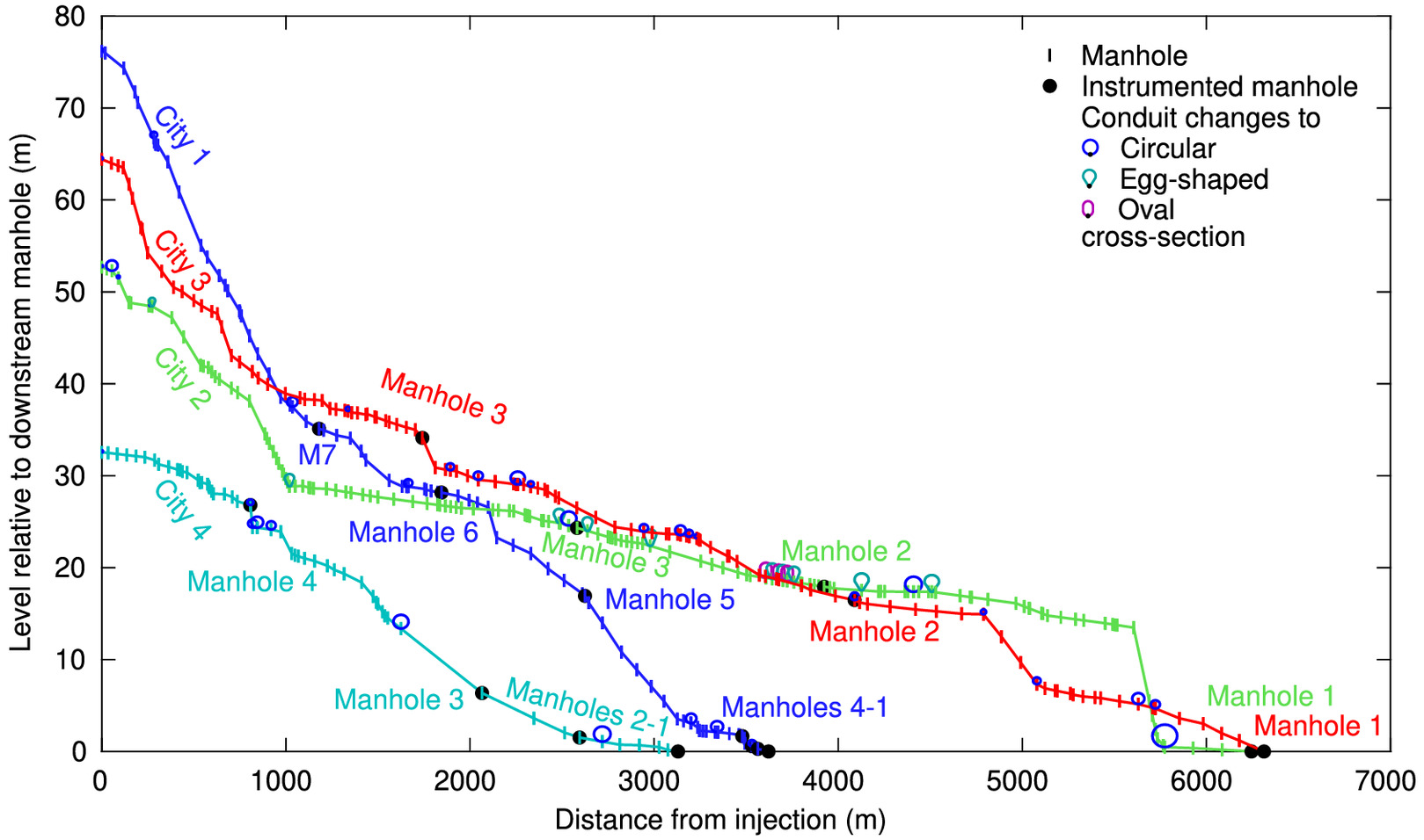
A fieldwork campaign, conducting fluorescent dye tracing in sewer networks, was carried out in 2021 and 2022 over a total of 23 days in four UK cities. The cities had between 3 and 8 measurement locations and the sites studied were between 3.6 and 6.3 km in length. The monitored sections of Cities 1 to 3 were linear with injections at the top of the network. While City 4 had measurements along a linear path, it also had the most complex set of experiments with injections on four different branches of the network. Across all four cities, there was a range of pipe diameters, between 225 and 2,450 mm, with circular, oval, and ‘egg-shaped’ concrete cross-sections (Innovyze Inc. 2022). An overview of the Cities is given in Table 1 and long sections are shown in Fig. 1. The geometry of these networks was available from validated InfoWorks hydrodynamic sewer models.

Table 1. Overview of study sewer networks

City	Number of monitoring locations	Length (km)	Primary conduit shape	Pipe diameter (mm)			Slope (1 in X)			Mean discharge ( $L / s$ )
City	Number of monitoring locations	Length (km)	Primary conduit shape	Min/median/max			Min/median/max			Mean discharge ( $L / s$ )
1	8	3.6	Circular	300	825	1,200	826	69	7	56
2	3	6.2	Egg	225	1,000	2,450	3,000	311	11	465
3	3	6.3	Circular	225	525	1,400	2,700	148	11	188
4	4	3.1	Circular	225	885	1,650	2,500	112	5	103

Source: Reproduced from Guymer et al. (2022), under Attribution 4.0 International (CC-BY-4.0) license (https://creativecommons.org/licenses/by/4.0/).

Fig. 1. City long sections with 50:1 vertical exaggeration. Changes in conduit cross section are drawn above the manhole where they change, scaled relative to each other. [Reproduced from Guymer et al. (2022), under Attribution 4.0 International (CC-BY-4.0) license (https://creativecommons.org/licenses/by/4.0/)].

The fluorescent dye tracing was carried out using up to eight Turner Designs Cyclops-7F submersible fluorometers (Turner Designs Inc., San Jose, California) attached to Precision Measurement Engineering submersible Cyclops-7 loggers (Precision Measurement Engineering, Inc., Vista, California), configured to log at 5-s intervals. Between 1 and 50 mL of dye, diluted into one litre of distilled water, was poured into the dry weather channel of an upstream manhole as a pulse injection. Dye volume was increased with increased distance and dilution to the furthest monitoring location. The dye used was Rhodamine WT (National Center for Biotechnology Information 2022) in a 20% solution obtained from Town End (Leeds) plc. (Leeds, UK). A temperature-dependent fluorometer calibration (Smart and Laidlaw 1977) was carried out, described in Appendix S1 and Fig. S1.

Initial fixed installation of the fluorometers to the side wall of the sewer often resulted in excessive ragging or the probe not being fully submerged. Upon switching to securing the probes by chain and laying them in the main channel, to allow more freedom of movement, ragging almost completely ceased. In instances where the water depth was insufficient, a small temporary weir was installed to submerge the probe further. Two fluorometers were installed in the furthest downstream manhole (Manhole 1) of City 3 to check on instrument installation (side wall fixture versus chained) and the robustness of the measurement system. More detailed guidance on conducting dye tracing in sewers is provided by Turner Designs Inc. (2022a).

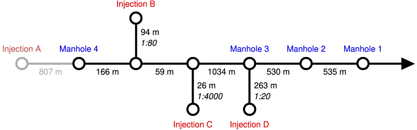
A unique aspect of the fieldwork is the multiple simultaneous dye injections carried out on the main leg and three side branches of the City 4 sewer network. This experiment was carried out twice, once with a single injection and once with a double injection at a 15-minute interval. A schematic of this network is provided in Fig. 2, showing the four injection and four monitoring manhole locations.

Fig. 2. The branched network of City 4 used for multiple simultaneous injections, slopes are given in italics. The grayed-out section was not modeled.

Simultaneous in situ flow monitoring was ongoing in City 1 at three of the manholes using Detectronic MSFN S2.5T area velocity flow meters (Detectronic Limited, Colne, UK). These recorded data at two-minute intervals. A 10-minute moving average was applied to the data to smooth out rapid oscillations. Matching discharge for a trace was calculated as the mean discharge from the start to the end of the trace.

Analysis Methods

The analyses undertaken in this paper, described in this section, are as follows:

1.

Process the concentration data recorded during the fluorescent dye tracing fieldwork to calculate discharge, travel time (velocity), and dispersion coefficient.

2.

Use the calculated discharge, in addition to network geometry, as the input to a simplified hydraulic model to estimate conduit characteristics (flow depth, hydraulic radius, etc.) at the time of the dye trace for each conduit between each upstream and downstream measurement location.

3.

Convert the individual conduit characteristics to single reach unified characteristics suitable for comparison to the measured dispersion coefficients and perform a regression analysis to identify a dispersion coefficient predictor.

4.

Investigate the multiple simultaneous injections and source localization using simplified hydraulic and solute transport modeling.

Concentration Data Processing

All recorded concentration profiles have been preprocessed. Times were corrected for logger clock drift and the data were temperature corrected. Visual inspection was used to identify background concentrations, which were subtracted, and then calibration was applied. A moving average was temporarily applied to reduce the impact of noise and the times of 1% of the peak concentration of the smoothed data were used to identify the start and end of the trace and trim the data record. In some instances, the start or end of the trace was manually defined due to poor quality data or traces overlapping due to injections too close together in time. The traces used for analysis were those judged to be of good quality, exhibiting low noise and a consistent scale with other traces from the same injection. Discharge from the recorded dye traces was calculated by equating the mass passing the fluorometer with the known mass of injected dye assuming perfect mass recovery. i.e.,

Q = v_{o} / \int c (x, t) d t

, where

v_{0}

is the volume of injected neat dye in

ppb . m^{3}

(Fischer et al. 1979).

To determine the travel time (velocity) and dispersion coefficient, pairs of upstream and downstream traces were identified for each injection, and then optimization of the routing solution to the 1D ADE was applied. The routing solution is given by

c (x_{2}, t) = \int_{γ = - \infty}^{\infty} \frac{c (x_{1}, γ) U}{\sqrt{4 π D_{x} \bar{t}}} \exp [- \frac{U^{2} {(\bar{t} - t + γ)}^{2}}{4 D_{x} \bar{t}}] d γ

(2)

where

c (x_{1}, t)

and

c (x_{2}, t)

are the temporal concentration profiles upstream and downstream at locations

x_{1}

and

x_{2}

,

\bar{t}

= travel time (the difference in centroids between the upstream and downstream profile), and

γ

= integration variable representing time (Fischer et al. 1979). By substituting an upstream concentration profile into Eq. (2), least-squares optimization may be performed comparing measured and predicted downstream concentration profiles to obtain the best-fit

U

and

D_{x}

(Guymer and O’Brien 2000), with

\bar{t} = (x_{2} - x_{1}) / U

. This was achieved using the MATLAB lsqcurvefit function (MathWorks Inc. 2022). The data were mass-balanced before optimization to comply with the implicit mass balance in Eq. (2). Although it is possible to calculate

\bar{t}

,

U

, and

D_{x}

between the injection and the most upstream measurement location, this has not been carried out due to uncertainties regarding the manual injection and very low discharges at the upper reaches of the network.

Similarity (goodness-of-fit) between predicted and measured values has been quantified using the

R_{t}^{2}

function:

R_{t}^{2} = 1 - \frac{\sum_{i = 1}^{N} {(\hat{y_{i}} - y_{i})}^{2}}{\sum_{i = 1}^{N} y_{i}^{2}}

(3)

where

\hat{y}

and

y

= predicted and measured values respectively (Young et al. 1980). An

R_{t}^{2}

value of 1.0 indicates perfect agreement, while a negative value indicates no agreement.

R_{t}^{2}

provides a robust comparison of measured and predicted concentration profiles (Sonnenwald et al. 2013).

Simplified Hydraulic and Solute Transport Model

To evaluate the dispersion coefficient while considering variations in pipe diameter and discharge, and to investigate source localization, a hydraulic and solute transport sewer network model was required that allows the prediction of conduit hydraulics and downstream concentration profiles. While the Saint-Venant equations typically used in commercial hydrodynamic modeling packages (e.g., Innovyze Inc. 2022) can be solved quickly (e.g., Li et al. 2022), in this case, the additional complexity introduced by requirements for a continuous geometry and the desire for rapid model execution for exploration and optimization led instead to the development of a simplified many-to-one network modeling approach. The simplified hydraulic and solute transport model utilizes Manning’s equation to estimate pipe velocities from discharge and Eq. (2) to model solute transport. Thus, the model only requires network geometry (pipe lengths and connections), flow rates, dispersion coefficients, and upstream concentrations. The hydraulic portion of the model calculates the velocity for each pipe, then the solute transport portion uses that velocity and a dispersion coefficient to route upstream to downstream concentrations, where downstream concentrations are diluted according to the ratio of flows calculated by the hydraulic portion. The model is described in more detail in Appendix S2.

Flow rates were taken where possible from the dye tracing results at upstream and downstream manholes. Where discharges calculated from tracing were unavailable (e.g., intermediate manholes), scaled mean daytime (9 a.m. to 6 p.m.) discharges from the available InfoWorks hydrodynamic sewer models were used.

Reach Unified Parameters

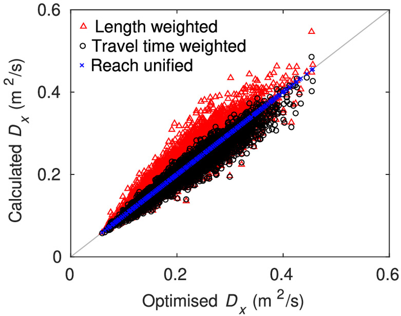
Longitudinal dispersion is often expressed as functions of parameters such as velocity, pipe diameter, surface width, slope, hydraulic radius, and flow depth (Fischer et al. 1979). The complexity of associating measured dispersion coefficients in sewers to these parameters is increased due to nonuniformity throughout the measurement reach. Rieckermann et al. (2005) suggested that length-weighted parameters could be used. Models of randomized reaches consisting of multiple pipes in series were created using the simplified modeling approach outlined in the previous section with a basic predictor of dispersion. Velocity and dispersion coefficient for the entire reach were found using least-squares optimization of Eq. (2). Although reach mean velocity calculated according to travel time weighting the velocity in each pipe (

U = \sum_{i = 1}^{N} U_{i} {\bar{t}}_{i} / \sum_{i = 1}^{N} {\bar{t}}_{i}

) was found to agree with the optimized velocity, neither length nor travel time weighted dispersion agreed with the optimized dispersion coefficient. Similarly, neither weighting approach described the other parameters, e.g., flow depth. As neither weighting approach can be used to relate dispersion coefficients over multiple pipes, as measured experimentally, to known network geometry, a new reach unified approach has been developed.

Eq. (2) may be substituted into itself to reveal that the equivalent unified longitudinal dispersion coefficient of a reach consisting of

N

multiple subreaches is given by:

D_{x} = \frac{{(\sum_{i = 1}^{N} U_{i} {\bar{t}}_{i})}^{2} \sum_{i = 1}^{N} (D_{x, i} {\bar{t}}_{i} \prod_{j = 1, j \neq i}^{N} U_{j}^{2})}{(\prod_{i = 1}^{N} U_{i}^{2}) {(\sum_{i = 1}^{N} {\bar{t}}_{i})}^{3}}

(4)

D_{x}

for a whole reach found optimizing Eq. (2) is compared to average sub-reach input

D_{x}

calculated using length weighting, travel time weighting, and Eq. (4) in Fig. 3. Both travel time weighting and Eq. (4) are improvements upon length weighted averaging, with reach unified

D_{x}

calculated using Eq. (4) showing perfect agreement with optimized

D_{x}

.

Fig. 3. Length weighted, travel time weighted, and reach unified dispersion coefficients compared to reach optimized dispersion coefficients. Line is line of equality.

Assuming that longitudinal dispersion is a function of velocity (Taylor 1954), then

D_{x} = k U

, where

k

is a constant, may be substituted along with the travel-time weighted velocity into Eq. (4) to obtain a relationship for reach unified parameters:

k = U \frac{\sum_{i = 1}^{N} k_{i} {\bar{t}}_{i} / U_{i}}{\sum_{i = 1}^{N} {\bar{t}}_{i}}

(5)

Eq. (5) is the equivalent of Eq. (4) for other parameters such as hydraulic radius. It is an alternative to length or travel time weighting, describing a reach unified value between two locations representative of several conduits with varying characteristics. When reach unified parameters are used predictively, it is reach unified

D_{x}

that is predicted, enabling the comparison between reaches with nonuniform characteristics and experimentally determined dispersion coefficients. This comparison has been carried out using a log-transformed multiple linear regression analysis (Gelman and Hill 2006) of reach unified parameters and experimental dispersion coefficient fit through the origin. This was achieved using the MATLAB regress function (MathWorks Inc. 2022).

Results and Discussion

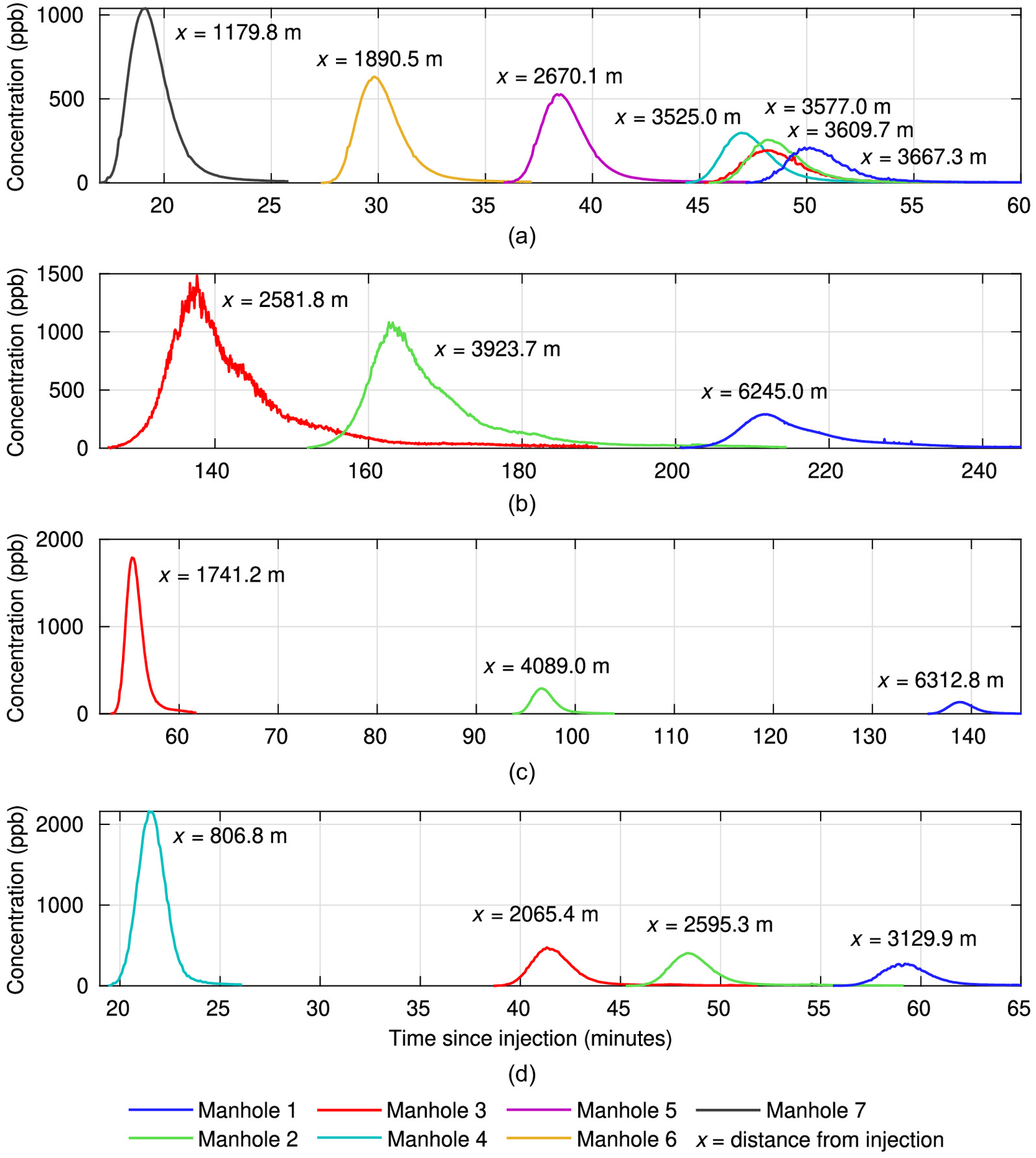
Of 191 dye traces recorded from 42 injections, 95 were suitable for analysis, providing the largest single data set of dye traces in sewers available, to date. 31 traces were off-scale due to being too close to the injection location and thus unusable, while the remaining traces were of insufficient quality. Example good quality results from injections in each City are shown in Fig. 4, with low noise and decreasing peaks downstream. Every monitoring location is represented except for the furthest upstream location in City 1 (Manhole 8), which never recorded a good trace. As evidenced by that absence, not all instruments recorded a good signal for every injection, and as a result, some injections are missing some sites. The additional noise at Manhole 3 of City 2 is typical of flow aeration affecting the measurement. In general, the profiles are Gaussian in shape, providing evidence of full cross-sectional mixing and sufficient time to reach equilibrium. The longer tails observed in City 2 at all three monitoring manholes are consistent with a very low discharge at the injection manhole stretching the input profile. In City 1, a storage tank between Manholes 4 and 3 combined with clock sync issues and very short pipe lengths has resulted in uncertainties in first arrival time at Manholes 3 and 2. The full set of recorded data are available in Guymer et al. (2022).

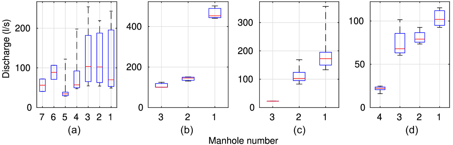
Fig. 4. Recorded traces from an injection at the most upstream location of (a) City 1; (b) City 2; (c) City 3; and (d) City 4, and manhole distances from the injection. Manhole 1 is the furthest downstream.

Discharge

Fig. 5 shows the distribution of calculated discharges, which almost always consistently increased downstream. Variability between repeated injections scales with discharge, explained by fluctuations in network use/flow conditions. The calculated discharge varies significantly in City 1 as the result of rainfall on one of the fieldwork days. The discharges observed are typical of moderate-sized catchments on the order of 10,000 thousand homes (Lawson et al. 2018). Out of four injections with good quality replicated measurements where two fluorometers were installed in Manhole 1 of City 3, the percentage difference in discharge between the two instruments ranged between 2% and 14%, with a mean of 8%. If the traces that show possible indicators of ragging are ignored, this drops to less than 5%, reflecting limitations of the measurement system depending on instrument location.

Discharges calculated from the dye tracing are compared to the matching in-situ flow meter measurements in Fig. 6. Approximately half of the flow meter measurements fall within the 8% error boundary of the dye calculated discharge previously suggested. Some of this variability is possibly due to imperfect dye injections. During rainfall, the flow meter at Manhole 1 reported less flow than at the upstream Manhole 3. Some error is expected in the flow meter readings as a result of a long installation period (months) where at least one instrument was replaced due to corrosion. Area-velocity flow meters are also sensitive to the build-up of sediment, surface level fluctuations, and the assumed area-velocity relationship.

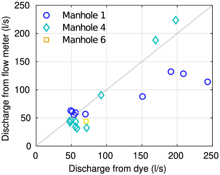
Fig. 6. Discharges calculated from dye tracing compared to metered discharges in City 1, $R_{t}^{2} = 0.873$ . Line is a line of equality.

The higher calculated discharges during rainfall may in part be the result of higher velocities encouraging the resuspension of previously settled sediments, increasing the effects of sorption and turbidity (Blaen et al. 2017). Under normal conditions, while sorption is possible due to the presence of, e.g., sediments, error in estimated hydraulic parameters in channels tends to be on the order of 1% as dye degradation occurs much less rapidly than the length of experiments (Runkel 2015; Turner Designs Inc. 2022b). Similarly, if operating to design standards, dry weather infiltration and inflow should be on the order 50 times less than measured flows (WRC 2012) and, in general, additional flow should dilute the dye, resulting in a correct higher measurement of discharge. Unfortunately, it was not possible to check on the effects of sorption, etc., during this study due to time and field constraints. Neither sorption, mass-recovery/degradation, nor infiltration/inflow should impact estimates of travel time or dispersion as it can reasonably be assumed, in line with the frozen cloud approximation (Fischer et al. 1979), that these processes occur much less rapidly than flow past the fluorometer.

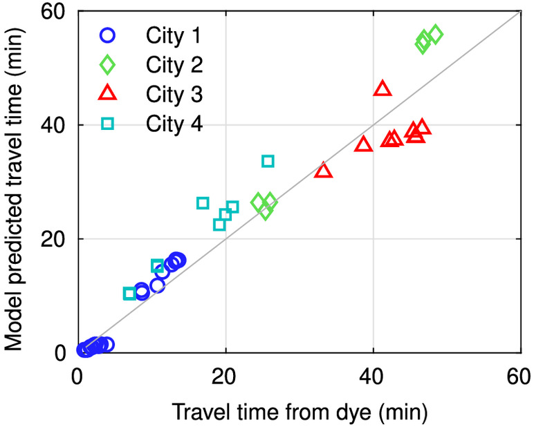
Simplified Model Predicted Travel Times

Fig. 7 compares calculated travel times with travel time predicted using the simplified modeling based on calculated discharge. Half of the predicted travel times fall within 20% of the measured travel time. Relative error increases as reaches get shorter, suggesting a consistent over-estimate in travel time regardless of reach length. For reaches over 100 m, the mean error in predicted travel time is 18%. This error may be due to the assumptions of steady-state and treating each pipe individually, in addition to imperfect network knowledge, e.g., limited estimates of roughness. The simplified model predicts travel time reasonably well with

R_{t}^{2} = 0.971

, suggesting the known network geometry reflects the buried infrastructure and that the model represents the hydraulics. Hence, the use of the simplified model is considered suitable as a tool for further investigation of dispersion within sewer networks.

Fig. 7. Simplified model predicted travel times compared to travel times calculated from dye tracing, $R_{t}^{2} = 0.971$ . Line is a line of equality.

Longitudinal Dispersion in Sewers

Dispersion coefficient and mean velocity were optimized from 44 trace pairs using Eq. (2) (shown in Fig. S2). Mean

R_{t}^{2}

was 0.994 with a standard deviation of 0.007, indicating that all dispersion coefficients describe the data well, confirming the applicability of a Gaussian transfer function description of mixing in sewers. Velocities ranged from 0.25 to

1.70 m / s

, with a mean of

0.87 m / s

. About one-quarter of these velocities fall below the

0.75 m / s

self-cleansing velocity suggested by WRC (2012). The longitudinal dispersion coefficient varied between 0.01 and

1.72 m^{2} / s

with a mean of

0.53 m^{2} / s

. The spread of the optimized experimental dispersion coefficients is shown in Fig. 8.

Fig. 8. Comparison of dispersion coefficients predicted using Eq. (6) and reach unified parameters to experimental longitudinal dispersion coefficients optimized from dye tracing using Eq. (2), $R_{t}^{2} = 0.610$ . Line is line of equality.

The City 3 injections with two fluorometers in Manhole 1 have been used to examine variability in the optimized dispersion coefficient. For the three replicated traces, the mean percentage difference in velocity was less than 1% and the mean percentage difference in dispersion coefficient ranged from 6% to 44% with a mean of 17%. In controlled laboratory pipe experiments, the percentage difference in dispersion coefficient between repeats ranged from less than 1% to 20%, with a mean of 5%, increasing with Reynolds number (Hart et al. 2021). Considering this, and that a 20% difference in

D_{x}

does not significantly impact a downstream prediction other than a small change in peak concentration (

R_{t}^{2}

changes less than 1%), the observed variability is expected.

The results obtained suggest dispersion increases with velocity, but that it is not solely a function of velocity. Pipe diameter, surface width, slope, hydraulic radius, and flow depth have been obtained for each pipe between the upstream and downstream measurement location using the simplified modeling and combined into a single reach unified value using Eq. (5). Of the parameters,

D_{x} / U

showed the strongest correlation with flow depth, hydraulic radius, and surface width. Performing regression analysis using the reach unified parameters, most of the possible predictors that were found performed equally well due to scatter in the data.

Of the theoretical predictors of

D_{x}

identified by Rieckermann et al. (2005), one of the best predictions was given by Sooky (1969), who performed a triple integral analysis of dispersion in an open channel with a circular segment cross section (a partially full pipe), assuming a vertical logarithmic velocity profile varying across the width of the pipe. They found

D_{x}

to be a function of hydraulic radius, channel width, and shear velocity. While this equation underpredicts experimental

D_{x}

here by approximately a factor of 10 (similar was also observed by Rieckermann et al. 2005), it can be modified and fit to the data to give:

D_{x} = 0.1 \frac{U W^{2}}{R}

(6)

where

W

is water surface width. This relationship maintains dimensionality and performs as well as any of the other predictors found using regression. Eq. (6) is not applicable for a pipe flowing full.

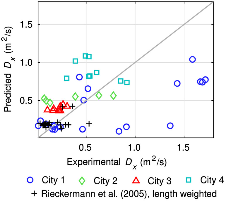
Fig. 8 shows the optimized experimental dispersion coefficients from the current study compared to predictions made using Eq. (6). Experimental dispersion values from Rieckermann et al. (2005) are also compared as a validation case, albeit using length weighted parameters in the absence of detailed network geometry. It is apparent that in the current study a larger range of dispersion coefficients has been found than that reported by Rieckermann et al. (2005), although there is a similar cluster of lower dispersion coefficients. Dispersion coefficient also tends to cluster by City, both the experimental and predicted values, suggesting some self-similarity in flow conditions and conduit geometry.

The tight clustering of dispersion coefficients for City 3 might be attributable to smaller more consistent pipe diameters, whereas the remaining cities had larger and more variability in pipe diameters. In City 1, the outliers with high optimized

D_{x}

and lower predicted

D_{x}

are from the very short reaches where there was some uncertainty in first arrival and hence travel time. Similarity between the predicted dispersion coefficients in each City is heavily influenced by similar velocities and hydraulic radiuses from repeat tests.

Rieckermann et al. (2005) suggested high dispersion values represent underperforming sewers. Some reaches have pipes with negative slopes and Sokáč and Velísková (2016) suggest these cause a backwater dead zone that would enhance dispersion. The reasonable performance of Eq. (6), showing a positive correlation between predicted and measured dispersion coefficient (

R_{t}^{2} = 0.610

), and its correct dimensionality, recommends it as a predictor of

D_{x}

in sewers. Combined with its simplicity, this has the potential to encourage its adoption when performing sewer network water quality modeling and improve those source localization methods relying on modeling results.

Multiple Simultaneous Injections

A simplified hydraulic and solute transport model (as described previously) of City 4 (Fig. 2) has been constructed to investigate the multiple simultaneous injections undertaken. The model covers every conduit between Manhole 4 and Manhole 1 as well as the conduits in the additional injection side branches. Discharges at the monitoring manholes have been estimated as the mean discharge from the single injection dye tracing work and discharges at the branches estimated from the available InfoWorks hydrodynamic sewer model.

The comparison of modeled and recorded concentrations resulting from the four simultaneous injections is shown in Fig. 9, where three downstream pulses were observed both in the recorded data and model prediction. Profile spread [described by Eq. (6)] appears visually similar. At Manhole 3 only the travel time of the last peak appears to be in good agreement, with the first two peaks offset within the error bounds of predicted travel time (Fig. 7). Further downstream, error in predicted travel time has increased, resulting in

R_{t}^{2}

values of 0.128,

- 0.662

, and

- 0.471

for Manholes 3, 2, and 1 respectively. The negative

R_{t}^{2}

values, due to the predicted travel times, suggest that the simplified hydraulic model may not be suitable for large applications as is, although an approximately 20% error on travel time and peak concentration is not unreasonable for an uncalibrated model utilizing only geometry and discharges. Some errors may also be attributable to differences between the modeled network geometry and actual buried infrastructure. Similar results were observed for the double injection.

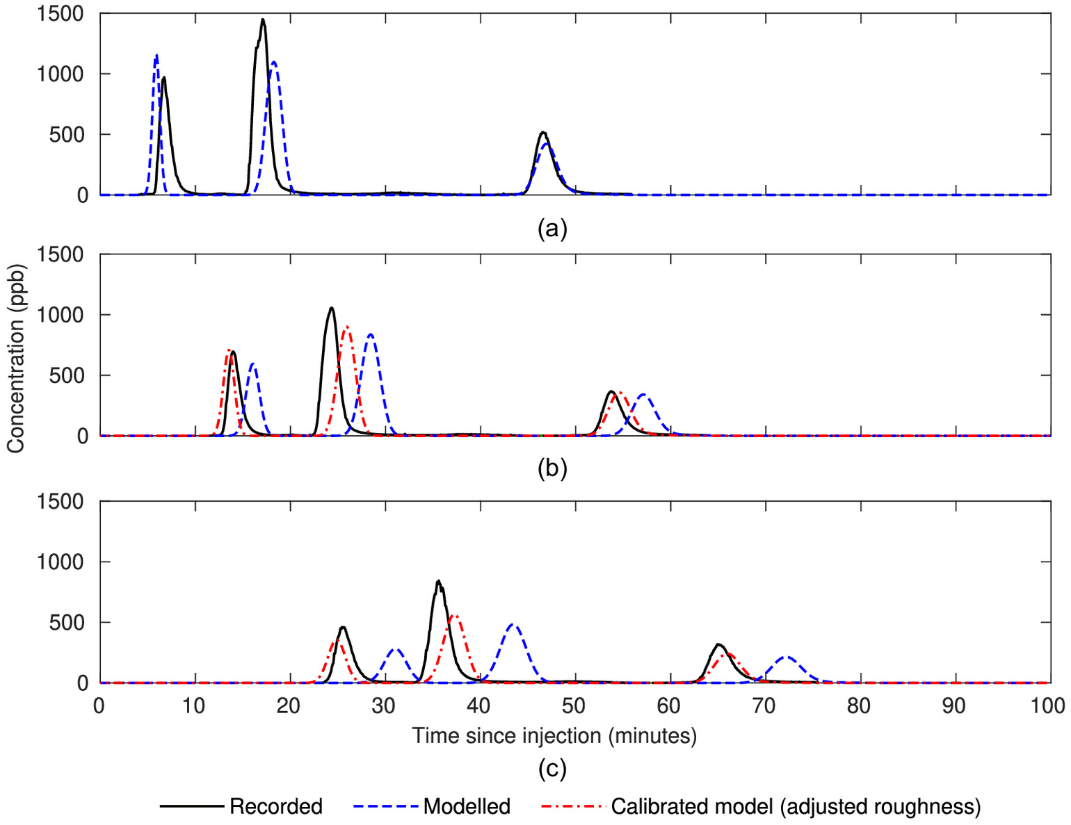
Fig. 9. Modeled and calibrated modeled concentrations compared to recorded concentrations downstream of multiple simultaneous injections into four branches of City 4 at: (a) manhole 3; (b) manhole 2; and (c) manhole 1.

To focus on investigating dispersion, a simple calibration has been applied by decreasing the roughness of the pipes downstream of Manhole 3 (

k_{s} / 10

or

n / 1.5

). This improves model agreement and suggests, in agreement with Mark (2005), the value of dye tracing as a tool for calibrating roughness. After calibration, all travel time predictions are within a few minutes and

R_{t}^{2}

values for the calibrated predictions are 0.138 and 0.467 for Manholes 2 and 1 respectively. Examining the last peak on its own, which has been in the flow for the longest amount of time and therefore experienced the widest variety of hydraulic conditions,

R_{t}^{2}

values are 0.950, 0.785, and 0.852, suggesting that the effects of dispersion are accurately modeled and that while the model does not produce a highly accurate prediction, it does represent the observed physical processes.

Although four injections were carried out for a single simultaneous input, only three peaks in concentration were measured (Fig. 9) when four were expected. This could easily be attributed to a misconnection or misunderstanding of the network geometry without further investigation. However, the model can be utilized to disaggregate the predicted concentration profile into contributions to total concentration from each injection location. This reveals that the second peak is formed of dye injected at injection locations B and C arriving near-simultaneously, as shown in Fig. 10. Verification is provided by the higher concentrations of the second peak predicted by the model matching that of the higher experimental measurement.

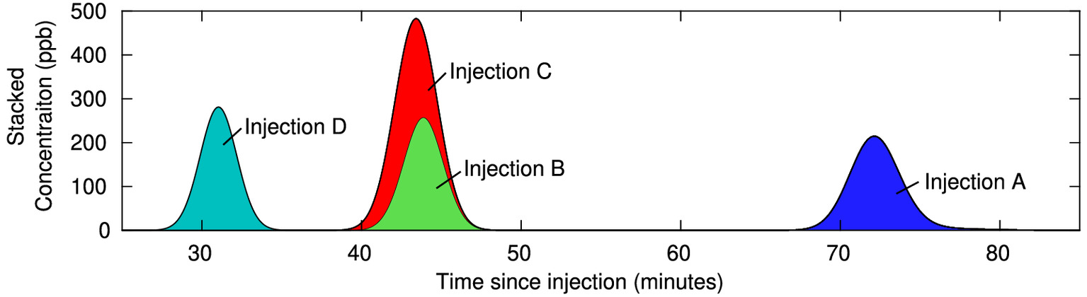
Fig. 10. Predicted contributions from each injection location stacked to predict concentrations at Manhole 1 [cf., Fig. 9(c)].

In retrospect, the coincident arrival of dye from injection locations B and C could have been anticipated considering the proximity of the two locations, being less than 150 m of conduit apart. This proximity was unfortunately unknown at the time of the fieldwork as these locations were selected on the day, with the constraints of safe accessibility and manholes that network data indicated were connected. The success of the model in identifying the dye from two locations arriving simultaneously highlights the power of physics-based numerical modeling in understanding observed behavior. Without the hydraulic and solute transport modeling, it would have been more difficult, if not impossible, to determine with confidence why only three peaks were observed from the four simultaneous injections.

Source Localization

The dye tracing and numerical modeling undertaken here have been done with consideration for source localization, i.e., finding the location of an event later monitored downstream. One approach to source localization based on a downstream measurement is that of matching a downstream record against a downstream prediction (Sokáč 2018; Grbčić et al. 2021). Zehnder (2021) identifies matching the spread of the recorded profile as a key factor. To do so requires an accurate description of dispersion, which we have shown to be obtainable from dye tracing. In general, understanding the relationship between the injection event and the monitored results of the event is essential, and this can be aided by the use of numerical modeling.

Some additional insight into source localization can be gained by assuming the cause of the event (e.g., an injection) is a short-duration (pulse) input. In which case, the recorded concentration distribution monitored at any given point in the network is a residence time distribution (RTD). An RTD describes the cumulative effects of dilution, advection, and mixing between the injection and measurement location (Levenspiel 1972). Following RTD theory, recorded downstream concentrations scale linearly with dilution and injection volume. If the short pulse occurs twice then two downstream responses are observed, i.e., the downstream response of an event is described by the convolution of the injection (which may be any arbitrary profile) with a network response (RTD).

Using numerical modeling, the RTD at a site can be calculated for every possible injection location, giving a sewer network “fingerprint,” similar to what is shown in Fig. 10. The measured downstream profile can then be compared to every RTD in the fingerprint to identify possible source locations. Fingerprint comparisons are limited by the instantaneous injection assumption since non-instantaneous injections, e.g., a more realistic time-distributed source, could produce similar/identical measured downstream profiles to a different instantaneous injection. Similarly, in a large network, two injection locations may have the same downstream profile, increasing uncertainty about the source location. Regardless, this approach could help to minimize possible source locations and thus the need for manual sampling throughout the network.

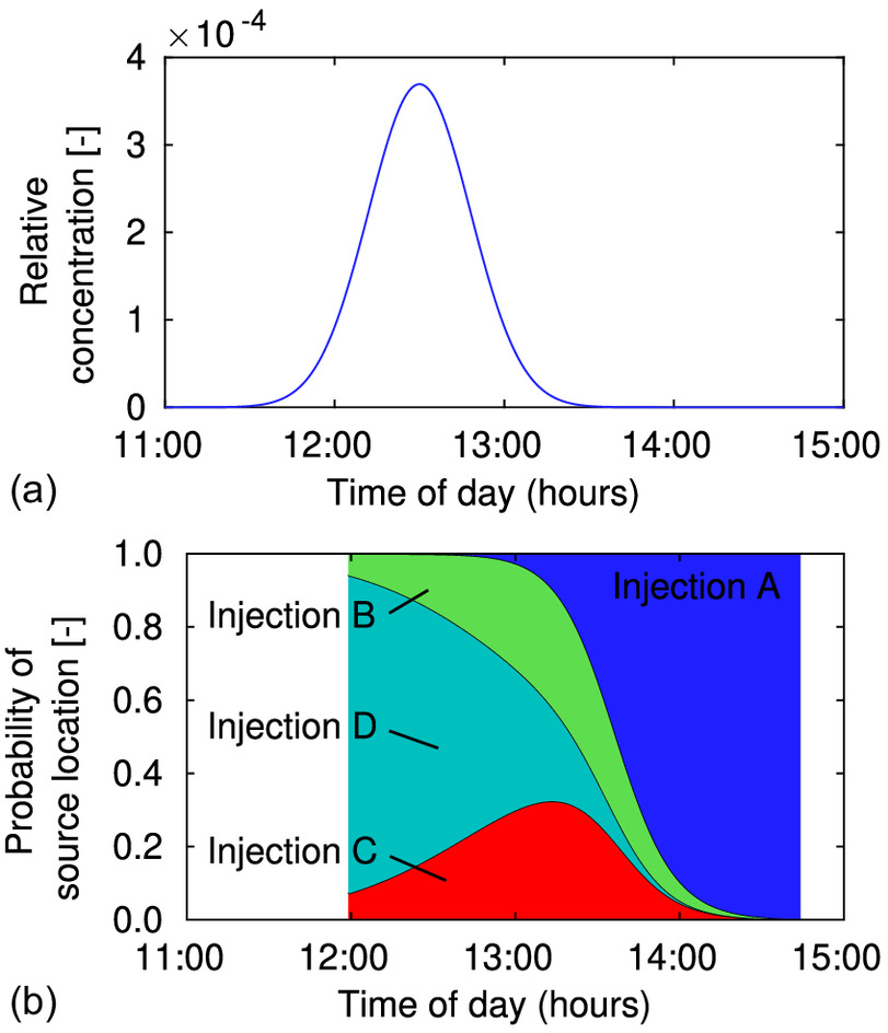
Unfortunately, to take best advantage of fingerprint comparisons, high-frequency continuous online monitoring is needed. Instead, the network fingerprint (each upstream manhole’s RTD) can be convolved (using the convolution integral; Levenspiel 1972) with a daily activity profile, producing estimates of downstream concentrations. Concentration contributions can be normalized by contribution to total concentration to produce a source location probability plot (SLP2), allowing the identification of possible sources of spot samples. This assumes that monitored events are related to human activity tied down to a time of day allowing the problem scope to be reduced. An illustrative daily profile is used to generate an example SLP2 in Fig. 11, with the contributions from each location shown in Fig. 10 (the City 4 Manhole 1 network fingerprint) convolved with a “lunchtime” profile [Fig. 11(a)]. The SLP2 in Fig. 11(b) is easily interpreted. The probability of a sample taken at 13:00 coming from injection locations A, B, C, and D are 3%, 29%, 30%, and 38%, while at 14:00 these probabilities are 89%, 5%, 5%, and 1%. This suggests the existence of optimal sampling times.

Fig. 11. Source location probability plot example: (a) illustrative lunchtime human behavior output profile; and (b) source location probabilities at City 4 Manhole 1 given time of day, assuming input into locations A to D according to the behavior profile.

In this way, the application of physics-based water quality modeling to source localization can help aid management decisions and maximize the inference possible from even a single measurement location. Such approaches enable small-scale, high-quality, cost-effective monitoring. Future work should focus on investigating and reducing the limitations of assumed steady flow, further validation, and the application of the approaches outlined here to more realistic scenarios using standardized hydraulic modeling tools.

Conclusions

Fluorescent dye tracing is a useful tool for the characterization of sewer hydraulics, confirmed by good quality tracing undertaken here in four UK sewer networks providing simultaneous measurement of discharge, travel time (velocity), and dispersion. This data can be used to improve descriptions of physical processes and modeling tools, and for validating water quality models in sewers.

The newly collected data has been analyzed with the aid of a simplified steady-state sewer network hydraulic and solute transport model and a new approach to averaging reach characteristics termed reach unified. Reach unification gives the equivalent longitudinal dispersion coefficient (

D_{x}

) and reach characteristics (e.g., hydraulic radius) for single ADE routing (as observed experimentally) to multiple ADE routings with varying

D_{x}

and reach characteristics carried out in series (as in a model). Reach unification has been used in reverse to better relate observed

D_{x}

with network geometry and produce a new, dimensionally correct, predictor of

D_{x}

.

Among the dye tracing carried out for this study were two, first of their kind, multiple simultaneous injections at four locations. A model of all four branches of this network was created and a comparison between it and the recorded dye traces revealed that the observed three peaks in response to four injections was due to two of the injections coinciding in the sewer. This demonstrates the value of physics-based modeling in understanding sewer network performance.

Consideration of the source localization problem suggests that residence time distribution (RTD) theory can be applied. A sewer network fingerprint is made up of the RTDs describing the possible concentration distributions observed at a monitoring location as a result of a pulse input at every upstream manhole. An assumed daily activity profile can be convolved with the fingerprint to produce a source location probability plot, which when compared with the time a sample was taken can be used to suggest possible sources. Further investigation of this approach is warranted.

Many studies investigating source localization focus on placing more sensors in better locations. In contrast, this paper explores the benefits of dye tracing, coupled with numerical modeling, to improve our understanding of network hydraulics and the underlying physical processes. These, in turn, improve the source localization that can be conducted with the data available from small-scale monitoring.

Notation

The following symbols are used in this paper:

$c$: concentration (ppb);
$D_{x}$: longitudinal dispersion coefficient ( $m^{2} / s$ );
$I$: reach or pipe index;
$k_{s}$: equivalent sand grain roughness (m);
$N$: number of;
$n$: Manning’s roughness coefficient ( $s / m^{1 / 3}$ );
$Q$: bulk discharge or flow rate ( $m^{3} / s$ );
$R$: hydraulic radius (m);
$t$: time (s);
$\bar{t}$: travel time (s);
$U$: mean streamwise velocity ( $m / s$ );
$u^{*}$: shear or friction velocity ( $m / s$ );
$W$: channel width at the surface (m); and
$x$: longitudinal position (m), with subscripts 1 and 2 indicating upstream and downstream respectively.

Supplemental Materials

File (supplemental_materials_joeedu.eeeng-7134_sonnenwald.pdf)

Download
374.63 KB

Data Availability Statement

The data created for this study are available in a repository online in accordance with funder data retention policies from (Guymer et al. 2022).

Acknowledgments

This work was supported by the EPSRC (Grant No. EP/P012027/1) and the UK Health Security Agency. The authors are grateful to Severn Trent Water, United Utilities, Welsh Water, Yorkshire Water, and their staff, for their assistance in accessing and monitoring networks, and to Joseph Milner, Environmental Monitoring Solutions, and others for their assistance in carrying out fieldwork. For the purposes of open access, the authors have applied a Creative Common Attribution (CC BY) license to any Author Accepted Manuscript version arising.

References

Adedoja, O. S., Y. Hamam, B. Khalaf, and R. Sadiku. 2018. “A state-of-the-art review of an optimal sensor placement for contaminant warning system in a water distribution network.” Urban Water J. 15 (10): 985–1000. https://doi.org/10.1080/1573062X.2019.1597378.

Abstract

Introduction

Field Work

Analysis Methods

Concentration Data Processing

Simplified Hydraulic and Solute Transport Model

Reach Unified Parameters

Results and Discussion

Discharge

Simplified Model Predicted Travel Times

Longitudinal Dispersion in Sewers

Multiple Simultaneous Injections

Source Localization

Conclusions

Notation

Supplemental Materials

Data Availability Statement

Acknowledgments

References

Information

Published In

Copyright

History

Authors

Affiliations

Metrics

Citations

Download citation

Figures

Other

Share

Copy the content Link

Share with email

Share

Request Username

Create a new account

Change Password

Password Changed Successfully

Verify Phone

Congrats!