Abstract
The main objective of this work is to characterize the stress–strain relationship of cross-laminated timber (CLT) wall panels when loaded in compression and how different confinement mechanisms provide compression reinforcement for the CLT panels. CLT crushing tests were performed to define the behavior of CLT under compression up to the failure point, defined here as the strain at which the gross stress falls by 20% from the peak value. Testing included monotonic uniform compression experiments of five-ply CLT with specimens that were 0.457 m wide by 1.52 m long. The motion of the specimens perpendicular to loading direction was restrained at midlength to prevent buckling. Twelve specimens were tested, including six bare CLT specimens and six reinforced specimens of CLT—three with self-tapping screws while the other three with self-tapping screws and an additional U-shape steel plate at the bottom of the specimens. Various damage points were observed during the tests, including (1) point at the onset of damage (through visual observation and instrumental observation) (2) point of initiation of strength degradation, (3) point at which buckling occurs, (4) point at which 25.4 mm delamination was observed, and (5) failure point. Three axial compression stress–strain models were adopted, calibrated, and compared. Results indicate that a stress–strain model combining linear and cubic functions for the elastic and softening responses, respectively, captures well the CLT inelastic behavior under compression.
Introduction
Cross-laminated timber (CLT) is an innovative engineered wood product that consists of at least three orthogonal laminated layers bonded with structural adhesives. Compared to traditional light-frame wood walls and floors, CLT exhibits relatively high in-plane and out-of-plane strength and stiffness properties, improved dimensional stability, adequate fire resistance, and satisfactory thermal and sound insulation performance when integrated with a holistic design solution (Karacabeyli and Douglas 2013). Therefore, use of CLT has gained popularity in Europe, Japan, North America, Australia, and New Zealand for residential and commercial building applications (van de Lindt et al. 2019). When CLT is used within a lateral force-resisting system (LFRS), the most common applications include its use as floor diaphragms and shear walls. CLT panels are often combined with posttensioning steel cables/rods to form a rocking wall system, which provides self-centering ability after a seismic event. A comprehensive review on posttensioning of timber members and structures, including CLT, was conducted by Granello et al. (2020). In addition, several testing programs reported on the damage typically observed in rocking wall systems, which can include wall toe compression damage (Blomgren et al. 2019; Mugabo et al. 2021; Hashemi et al. 2017). As indicated in Busch et al. (2021), plastic deformations are permitted for maximum considered earthquake levels of design, which in the case of a CLT shear wall corresponds to wall toe crushing; acceptance limits of wall toe crushing can be found in Busch et al. (2021) for CLT panels used in posttensioned rocking shear wall applications. In certain cases, to limit the wall toe damage in compression, especially in high seismic regions, wall toe reinforcement can be used. Applications of CLT LFRS are not limited to design of new buildings as several retrofit and rehabilitation solutions have been proposed for existing buildings (e.g., Engleson 2019). In all the solutions mentioned previously, it is crucial to understand the compressive behavior of the wall toe.
The compressive stress–strain relationship of CLT is required to design and model CLT walls, especially rocking walls. A typical stress–strain model for CLT in compression is the elastic-perfectly-plastic (EPP) material model, which does not include the strength degradation behavior of the material. Thus, in studies that adopt the EPP model, the force-displacement response and moment-rotation models are not able to capture post-peak loss in strength observed in experiments (Akbas et al. 2017). To improve the accuracy in modeling, a fundamental understanding of the performance of CLT in parallel-to-major strength direction is imperative.
There have been several studies on the parallel-to-grain compression behavior of CLT panels (Ganey et al. 2017; Wei et al. 2019 He et al. 2020). Ganey et al. (2017) tested three-layer and five-layer CLT specimens in three directions to obtain material properties for CLT panels. Ten three-layer and two five-layer specimens were tested in the primary strength direction. The three-layer specimens were 278 mm tall, and their gross cross-section area varied from to . Meanwhile, the five-layer specimens were 511 mm tall, and the cross-section area ranged from 28,650 to . Based on the testing results, the modulus of elasticity and yield stress did not vary with the ratio of cross-sectional area to the height or number of layers. Wei et al. (2019) investigated the compression behavior of Canadian western hemlock CLT panels by testing three-layer specimens with the cross-section dimensions of 105 mm by 105 mm and lengths of either 210 mm or 420 mm. The effects of specimen lengths on the compression properties of the specimens were analyzed by a one-way analysis of variance (ANOVA). Results show that the length of specimens did not significantly affect the compression strength and modulus of elasticity. Although the size effect did not considerably influence the results in these studies, the dimensions of specimens were small and thus do not represent the structural sizes of CLT walls as used in real world projects. Wei et al. (2019) utilized experimental stress–strain curves to validate three axial compression stress–strain models. Wei et al. (2019) defined 60% of the peak stress as the stress at the elastic limit (), while the failure stress () was a post-peak stress at 90% of the peak. Most testing standards for wood-based materials [e.g., ASTM D4761 (ASTM 2019b) and Eurocode EN 408:2003] provide guidance for determining the compression strength (i.e., the ultimate stress ), but not for yield stress and failure stress. In the standards ASTM D4761 (ASTM 2019b), only the characteristic causing failure and its location are recorded. Therefore, there is a lack of definition of compressive yield stress and failure stress for wood-based materials in testing and no consensus on the definition of these stress points for modeling.
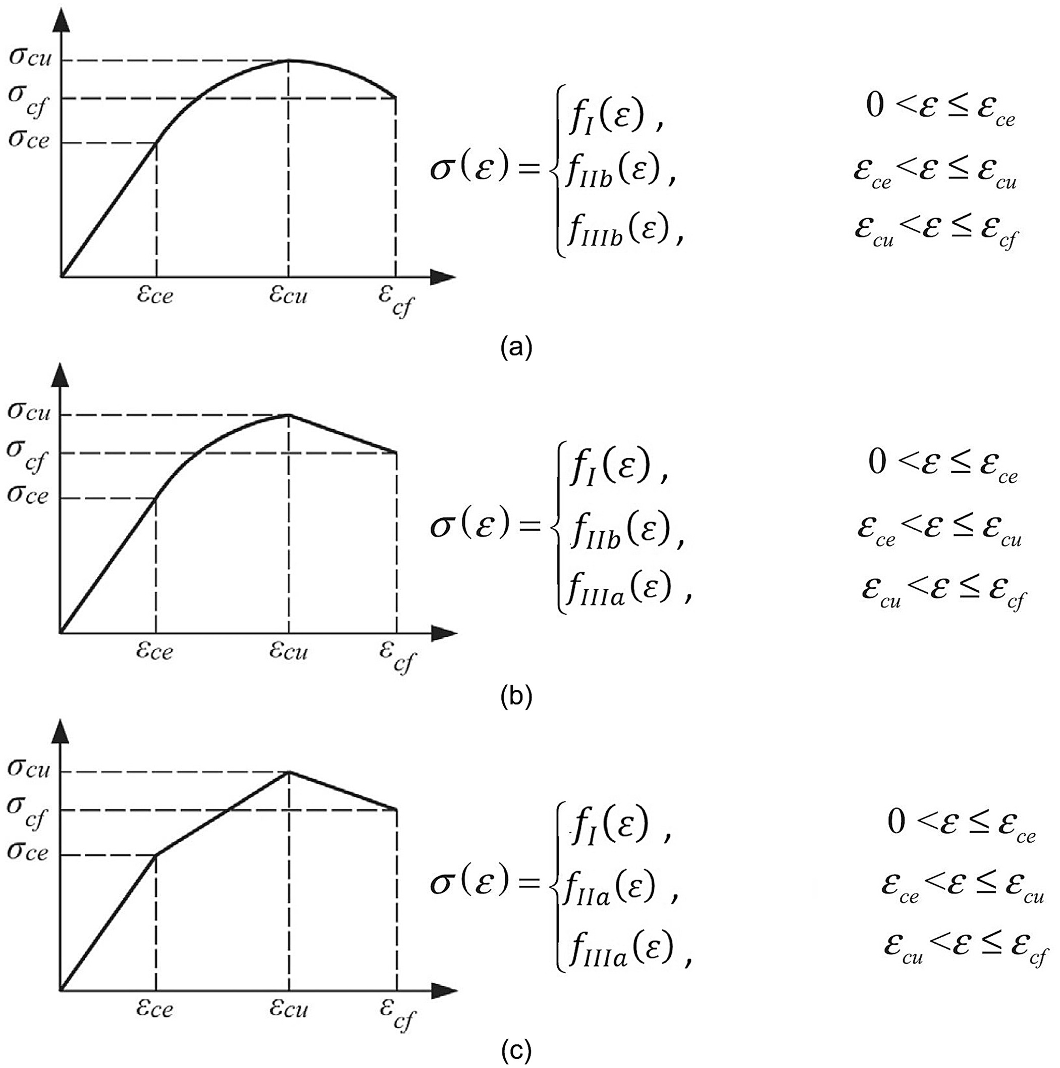
In terms of modeling the axial, unidirectional compression stress–strain behavior of CLT, Ganey et al. (2017) utilized an elastic-perfectly plastic material model. The yield stress was taken as the maximum stress the specimen achieved before losing its load-carrying capacity. Wei et al. (2019) developed three models for describing the wood axial compression stress–strain relationship (Fig. 1). A stress–strain curve can be divided into three segments, consisting of an elastic segment (or segment I), hardening segment (or segment II), and softening segment (or segment III). Segment I represent the elastic range of the stress–strain curve and it is limited by yield point . The hardening segment indicates the range beyond the yield point up to the ultimate point . The post-peak segment of the stress–strain curve is labeled as the softening segment and defined by ultimate point and failure point . All models share the same linear function for segment I and use either a linear function or quadratic function to describe segments II and III. The parameters of quadratic functions are determined based on a system of three equations.
The main objective of this paper is to characterize the stress–strain relationship of CLT wall panels when loaded in compression and how different confinement mechanisms provide compression reinforcement for the CLT panels. The paper presents an experimental program developed to characterize the compressive behavior of a series of large-scale CLT panels. The large-scale physical tests were driven by the need for testing data on the structural performance of building subassemblies of an award-winning project (Framework Portland Project 2017) and to increase the state of knowledge of mass-timber systems for building applications for broader use around the world. The panels were loaded under a displacement-controlled test beyond the peak load until the strength loss was greater than 20% of the peak load. In this study, the stresses derived from compression load were based on the gross cross-section area; therefore, they correspond to as gross stresses. The failure point in this study was defined as a post-peak point where its stress was 80% of the ultimate stress. In addition, the effect of reinforcements on the compression behavior is also analyzed with the integration of two reinforcement types that were subjected to the same testing protocols. The specimens with and without reinforcements were tested to characterize various damage points, which are represented by different stress–strain points, including: (1) point at the onset of damage (through visual observation and instrumental observation) (2) point of initiation of strength degradation, (3) point at which buckling occurs, (4) point at which 25.4 mm delamination was observed, and (5) failure point. Lastly, three axial compression stress–strain models are presented, calibrated, and compared.
Materials and Methods
Specimen Description
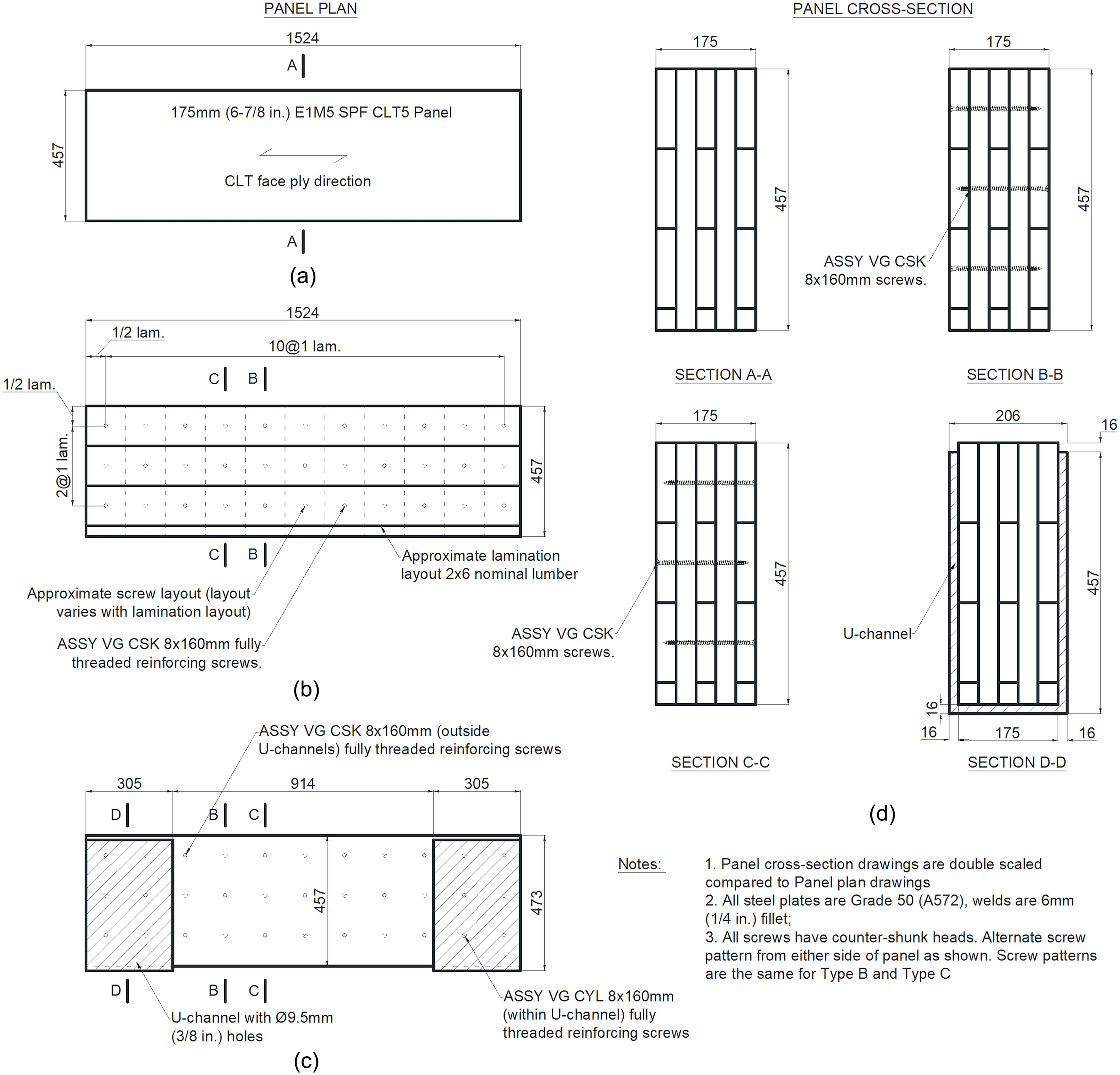
Twelve CLT panels were procured from a commercial manufacturer for this testing program. The panels were 457 mm wide, 175 mm thick, and 1,524 mm long (Fig. 2). The CLT panels used in the specimens are E1 grade per ANSI PRG 320-2019 (ANSI/APA 2019), including machine stress rated (MSR) spruce-pine-fir (SPF) longitudinal layers and No. 3 SPF transverse layers. Before shipping, a water repellent was applied to the end grains in the fabrication shop. The average moisture content of the as-received panels was 15.5%, measured by a pin-type moisture meter. The moisture content and dimensions of each specimen are shown in Table 1.
| Sample No. | Treatment type | As tested | Dimensions | ||
|---|---|---|---|---|---|
| MC (%) | L (mm) | W (mm) | T (mm) | ||
| 1 | Type A | 16.1 | 1,524 | 457 | 176 |
| 2 | 15.8 | 1,524 | 460 | 176 | |
| 3 | 16.1 | 1,524 | 457 | 177 | |
| 4 | 14.9 | 1,524 | 460 | 176 | |
| 5 | 15.3 | 1,524 | 460 | 176 | |
| 6 | 15.7 | 1,524 | 457 | 176 | |
| 7 | Type B | 14.8 | 1,524 | 457 | 176 |
| 8 | 15.2 | 1,524 | 457 | 176 | |
| 9 | 15.5 | 1,524 | 460 | 176 | |
| 10 | Type C | 15.4 | 1,524 | 457 | 176 |
| 11 | 16.0 | 1,524 | 457 | 176 | |
| 12 | 15.5 | 1,524 | 457 | 176 | |
Note: Type A: no reinforcement; Type B: self-tap screws (STS) reinforcement; Type C: STS and U-channels reinforcement; MC = moisture content; L = bare panel length; W = bare panel width; and T = bare panel thickness.
A total of twelve panels were tested. Six (6) panels, designated as type A [Fig. 2(a)], were tested without any reinforcement to provide the baseline values. Two reinforcement types, designated as types B and C, as shown in Figs. 2(b and c), respectively, were tested with reinforcements installed to prevent buckling of the fiber ends and provide confinement at the ends. Three specimens were tested for each of the reinforcement panel types.
The intent of the reinforcement was to enhance the post peak performance of the panels in compression. The application of the reinforcements was performed at the laboratory by specialized crewmembers. The type B panels were reinforced using ASSY VG CSK fully threaded screws (MTC Solutions 2020) drilled on the surface of the panels penetrating through the thickness. The type C panel reinforcement consisted of welded steel plates forming a U-section installed at either ends of the panel. Each U-section consisted of two (2) side plates and one (1) end plate, which were connected using 6 mm fillet welds, as shown in section D-D in Fig. 2(d). The CLT panels were not rounded at the edges. The plates consisted of Grade 50 [ASTM A572 (ASTM 2021)] steel. ASSY VG CYL fully threaded screws (MTC Solutions 2020) were used for segments with the U-section steel plates, while ASSY VG CSK screws were installed at the other location. The screws were pre-drilled with 9.5mm diameter holes on the side plates of U-section steel plates. The screw pattern is shown in sections B-B and C-C in Fig. 2(d) and was similar for both type B and type C panels.
Testing Methods
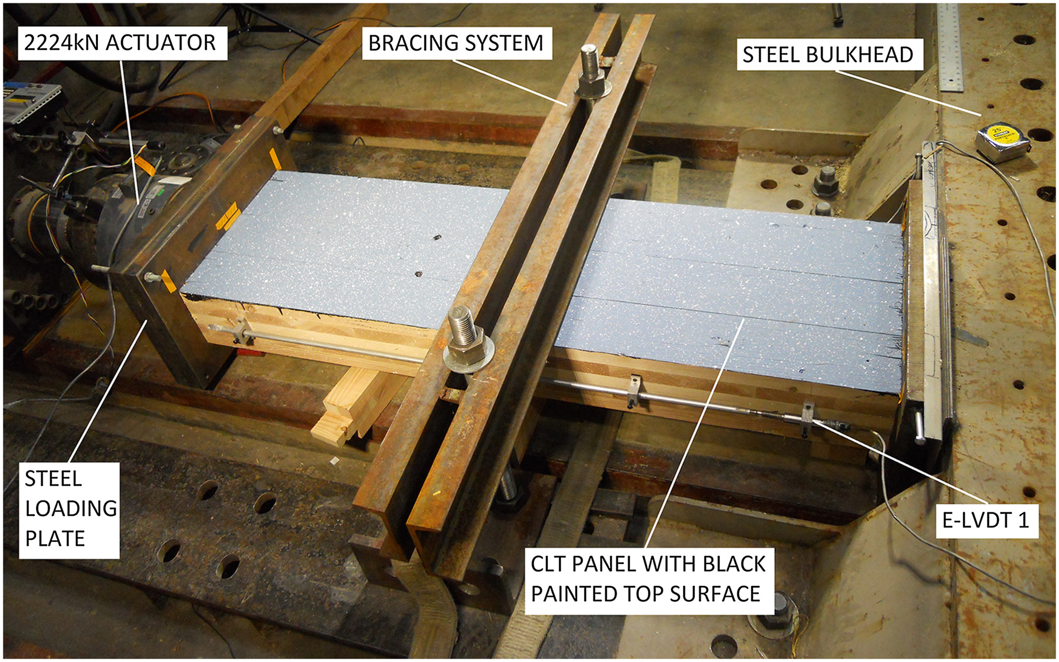
The experimental set-up and the instrumentation plan are shown in Fig. 3. The tests were performed horizontally to ease the material handling and for safety reasons. A digital image of the testing set-up is shown in Fig. 4. The set-up consisted of a 2,224 kN (500-kip) hydraulic actuator with a 508 mm (20-in.) stroke. The hydraulic actuator was braced to prevent uplift that could, in turn, produce out-of-plane loading. A steel bulkhead was used at the other end of the panel, which was bolted to the strong floor using four anchor points. Each anchor point included a set of four 25.4 mm diameter bolts. A steel plate was attached to the steel bulkhead that was connected to the base of the CLT panel to provide an even surface for the panel to react against. The CLT panel was placed on a timber block. On top of the panel and in line with the timber block, a buckling restraint mechanism consisting of C-channels and 19 mm all-threaded rods was installed, which is labeled as bracing system in Fig. 3. Frictionless surfaces were provided at the CLT panel to the timber block interface and the CLT panel to C-channels interface using two greased high-density polyethylene sheets. The alignment of the panels and the actuator load head were matched and checked using a laser level.
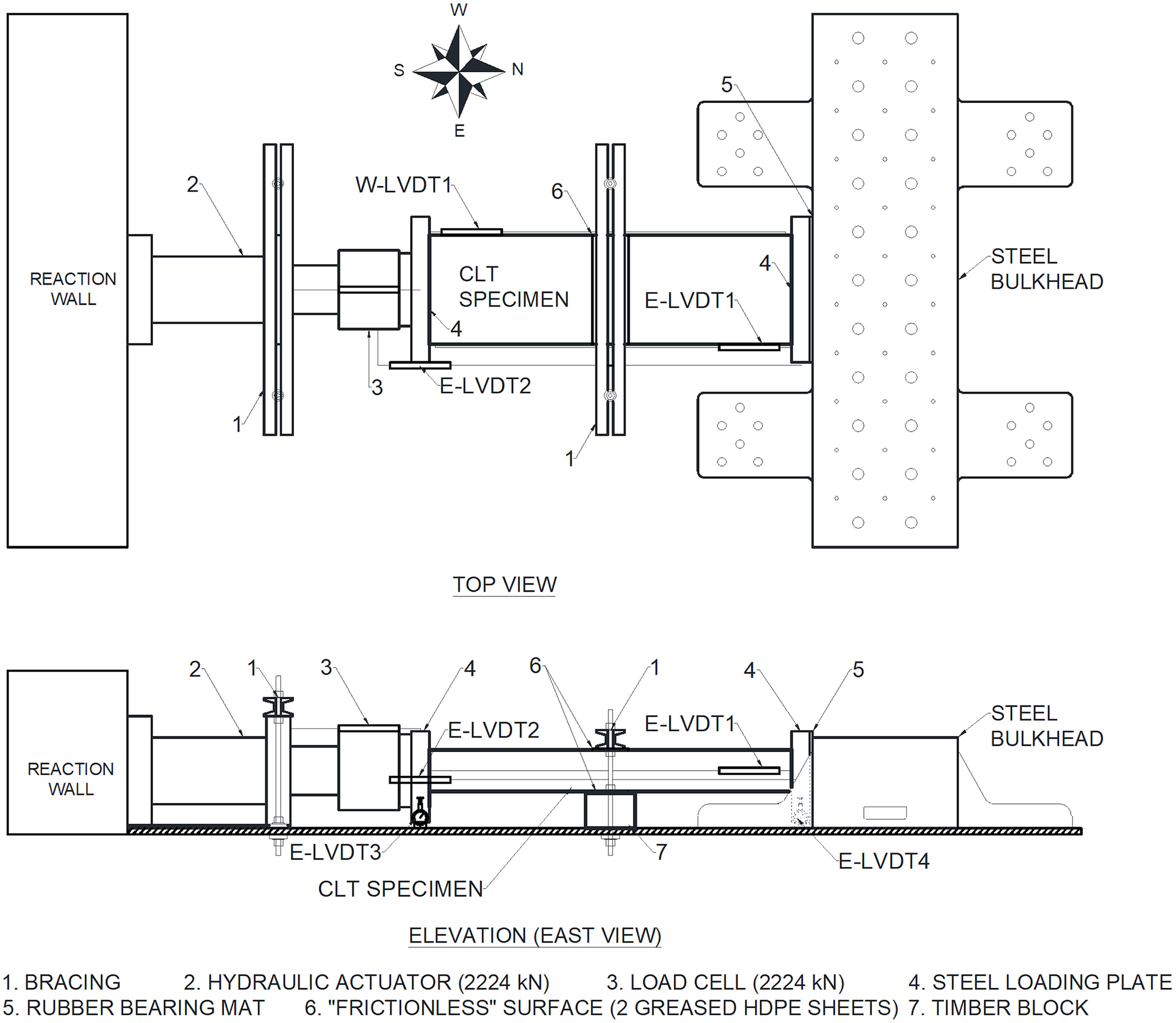
The instrumentation plan included a load cell, linear variable differential transducers (LVDTs), and digital image correlation (DIC) equipment. Two LVDTs were used on either side of the panel to measure the axial compression movement along the centerline of the panel, over a gauge length of 1,219 mm, shown as W-LVDT1 and E-LVDT1 in Fig. 3. To avoid destruction of the sensors these two LVDTs were removed after 80% of ultimate stress was reached post peak. A third LVDT was attached on the east side of a steel loading plate and measured the displacement between the plates at two ends of the specimen, shown as E-LVDT2 in Fig. 3. The range of the LVDTs was . On either side of the steel plates, LVDTs were used to measure the vertical displacement of the steel plates on the east side (E-LVDT3 and E-LVDT4) as shown in Fig. 3, and W-LVDT2 and W-LVDT3 on the west side (not shown in Fig. 3 for clarity of the figure). These latter four LVDTs had a measurement range of 12.70 mm, and were installed to measure out-of-plane movement to confirm if the out-of-plane motion was small to negligible.
The top surface of the panels was tracked using DIC and the DIC data was analyzed to obtain displacements and strain maps of the top surface. In the DIC setup, two cameras take images of the specimen at a predetermined time interval. The images taken when the specimen is under load are then correlated back to a baseline (initial) image to form a strain and displacement profile of the surface. To ensure that this tracking was performed accurately, the surface was painted black and speckled with white dots to provide a unique pattern and contrast (Fig. 4). In addition, the DIC system was calibrated to capture local deformations.
The actuator load and deflection of the load head, as well as the LVDT deflections, were continuously monitored and logged using an automated data acquisition system. Based on the monitored load and deflection data, load-deflection curves were generated for further analysis.
A monotonic load was applied to the CLT panel using a steel plate between the head of the CLT panel and the actuator. The test was performed under a constant displacement rate of 1.27 mm per minute. The test was continued until the load dropped more than 20% with respect to the measured peak load.
Mechanical Parameter Determination
As mentioned in the “Introduction” section, in this study, the stress is calculated as an engineering stress based on the ratio of the actuator load and the gross cross-section area. For convenience, the word stress is utilized in this study and refers to the gross stress or the engineering stress. The strains, which were determined from the measurement of W-LVDT1 and E-LVDT1 over a gauge length of 1,219 mm, are referred as west strain and east strain, respectively, and utilized to plot stress–strain curves. The strain derived from DIC data is labeled as DIC strain. Similar to Wei et al. (2019), a stress–strain curve is divided into three segments, including elastic segment, hardening segment and softening segment.
Several material parameters, including yield point, ultimate point, failure point, gross modulus of elasticity, and stiffness, were estimated from both east and west stress–strain curves and the mean results are presented in this paper. The yield point is a point on the stress–strain curve where the onset of local damage in terms of strain determined from DIC data, which will be discussed in the following section. The ultimate point is a point on the stress–strain curve where the stress is maximum. A point on the softening segment when the stress drops to 80% of the peak stress was defined as the failure point. The failure point was assumed to provide the compressive strain at which the panel suffered complete failure. This failure point was used as a majority of studies in timber engineering has used this based on ASTM E2126 (ASTM 2019a). The ultimate point and failure point were directly determined from the stress–strain curve. The gross modulus of elasticity (MOE) was determined by applying linear regression to a linear segment on a stress–strain curve obtained from the LVDT1 measurements. The points defining the linear segment are 20% and 50% of the ultimate stress for the lower and upper values. The instantaneous stiffness of each specimen was determined as the first derivative of a stress–strain curve, and the result was plotted as a stiffness-strain curve.
Failure Progression Observations
Failure progression was assessed during testing by tracking several damage indicators. The following damage points were determined, including: (1) point at the onset of damage (through visual observation and instrumental observation), (2) point of initiation of strength degradation (i.e., ultimate point where the stress reached its peak), (3) point at which buckling occurs, (4) point at which 25.4 mm delamination was observed, and (5) failure point.
The ultimate and failure points were determined from the stress–strain results, as indicated in the previous section. Three approaches were used to capture the other damage points (onset of damage, buckling, 25.4 mm delamination) in the failure progression. These approaches were stiffness observation, DIC estimation, and visual estimation. These approaches were utilized independently or combined to determine damage points. The description of these approaches is presented hereafter.
The stiffness observation approach is implemented by determining the tangent stiffness for the specimens. The tangent stiffness was plotted against the strains and two points identified, including the peak stiffness point and the 90% of the post peak stiffness point. The latter was defined as the onset of damage.
DIC observation is based on DIC data recorded during the test at an equal time interval of one second. These data were processed to produce DIC strain maps, which allowed to observe the change in surface strain during testing. These strain maps provide valuable information about the condition of the specimen surface. Quantitatively, the DIC technique can provide instantaneous strain at any point or an average strain over a selected area. Observing the DIC strain maps helps to determine when and where the first surface local strain reached to 3,000 microstrain over an area of 50.8 mm diameter circle, which indicated an onset of local damage in terms of strain and as discussed in the “Test Results and Discussion” section, correlated with average strain at peak load.
The visual estimation approach involves visually observing the damage visible by the naked eye during testing and correlate the observed damage with testing notes and the stress–strain curve. Correlation of visual observations and stress–strain curve was used to determine the onset of damage based on visual observations, the point at which buckling occurs, and the point at which 25.4 mm delamination occurs. In addition, DIC data were combined with visual assessment (photos and videos recorded during testing) and testing notes to report on the failure progression.
Engineering Stress–Strain Models
In this paper, the three models shown in Fig. 1 are adopted, which are all based on models proposed in Wei et al. (2019) with minor modifications. For example, the hardening segment in Wei et al. (2019) did not provide a smooth transition from the elastic segment, and therefore, a cubic function is proposed in this study. The details of the stress–strain curve models are discussed as follows.
In all three models shown in Fig. 1, the stress in the elastic segment () is expressed as a linear function given by:where = gross modulus of elasticity (MOE) determined from the experiment; and = elastic compressive strain limit at yield point. The stress at the elastic compressive strain limit at the yield point is expressed as .
(1)
For the hardening segments (), a linear expression and a cubic expression are considered as shown in Fig. 1 and given by:wherewhere, are strain and stress coordinates corresponding to the ultimate point. For the softening segment (), either a linear function or a quadratic function are used. These are given by:wherewhere = strain and stress coordinates corresponding to the failure point.
(2)
(3)
(4)
(5a)
(5b)
(5c)
(5d)
(6)
(7)
(8)
(9a)
(9b)
(9c)
The goodness-of-fit of the numerical models to the mean experimental results of each treatment type is determined using the root mean square error () and R-squared () coefficient of determination, which are given bywhere is the number of data points in the mean experimental stress–strain curve.
(10)
(11)
is a mean experimental stress corresponding to the th strain data point () and given bywhere is the sample size of a treatment type, is an experimental stress of the th sample corresponding to .
(12)
is a predictive value obtained from a stress–strain model corresponding to .
is the mean stress value of all mean experimental data points given by:
(13)
Test Results and Discussion
Engineering Properties
Table 2 provides a summary of the test results from the experimental program. The mean peak load for the Type A CLT panels is 1,582.3 kN with a coefficient of variation (CoV) of 3.7%. The gross MOE has a mean value of 7,338 MPa and a CoV of 5.5%. The calculation of the MOE did not exclude the perpendicular laminations as the gross cross-section area was utilized in the calculation of average stress. The results of the type B and type C panels show an increase of the mean peak load to 1,706.8 kN and 1,741.5 kN, respectively, corresponding to a 7.9% and 10% increase with respect to the control panels (i.e., type A panels). The increases in mean peak load were statistically significant (, -test). Among the reinforcement solutions, there was no statistical difference between the peak loads for type B and type C treatments (, -test). An increase in the mean MOE was observed in the type C treatment, but not in the type B, where the type B group mean MOE was 7,242 MPa and the mean MOE of the type C group was 8,081 MPa. The difference in MOE between the reference and the type C group was significant (, ).
| Treatment type | Sample No. | Peak load (kN) | Bulk MOE (MPa) | Load (kN) | Onset of buckling | Load (kN) | Delamination. reaching 25.4 mm | ||
|---|---|---|---|---|---|---|---|---|---|
| Stress (MPa) | Displacement (mm) | Stress (MPa) | Displacement (mm) | ||||||
| Type A | 1 | 1,661.4 | 7,867 | 1,539.1 | 19.09 | 8.0 | 1223.3 | 15.17 | 11.2 |
| 2 | 1,587.6 | 6,929 | 1,352.3 | 16.71 | 9.6 | 974.2 | 12.04 | 17.8 | |
| 3 | 1,605.8 | 7,543 | 1,245.5 | 15.41 | 9.7 | 849.6 | 10.51 | 19.1 | |
| 4 | 1,491.9 | 6,798 | 1,316.7 | 16.31 | 9.3 | 1014.2 | 12.56 | 14.8 | |
| 5 | 1,541.8 | 7,460 | 1,276.6 | 15.80 | 10.5 | 960.8 | 11.89 | 21.0 | |
| 6 | 1,605.4 | 7,433 | 1,347.8 | 16.77 | 9.1 | 556.0 | 6.92 | 15.2 | |
| Mean | 1,582.3 | 7,338 | 1,346.3 | 16.68 | 9.4 | 929.7 | 11.51 | 16.5 | |
| CoV (%) | 3.7 | 5.5 | 7.7 | 7.74 | 8.9 | 23.7 | 23.62 | 21.0 | |
| Type B | 7 | 1,703.2 | 7,743 | 1,548.0 | 19.24 | 11.7 | 431.5 | 5.36 | 10.7 |
| 8 | 1,823.8 | 6,819 | — | — | — | 716.2 | 8.89 | 11.6 | |
| 9 | 1,593.4 | 7,164 | 1,316.7 | 16.27 | 8.6 | 431.5 | 5.33 | 12.8 | |
| Mean | 1,706.8 | 7,242 | 1,432.3 | 17.75 | 10.1 | 526.4 | 6.53 | 11.7 | |
| CoV (%) | 6.8 | 6.4 | 11.4 | 11.81 | 21.6 | 31.2 | 31.31 | 8.9 | |
| Type C | 10 | 1,716.1 | 7,998 | 1,338.9 | 16.68 | 13.9 | 827.4 | 10.30 | 23.9 |
| 11 | 1,704.6 | 8,184 | 1,321.1 | 16.39 | 12.2 | 676.1 | 8.39 | 17.8 | |
| 12 | 1,803.8 | 8,060 | 1,330.0 | 16.55 | 13.2 | 920.8 | 11.46 | 29.8 | |
| Mean | 1,741.5 | 8,081 | 1,330.0 | 16.54 | 13.1 | 808.1 | 10.05 | 23.8 | |
| CoV (%) | 3.1 | 1.2 | 0.7 | 0.86 | 6.4 | 15.3 | 15.42 | 25.2 | |
Note: Bold values indicate mean and COV of the group.
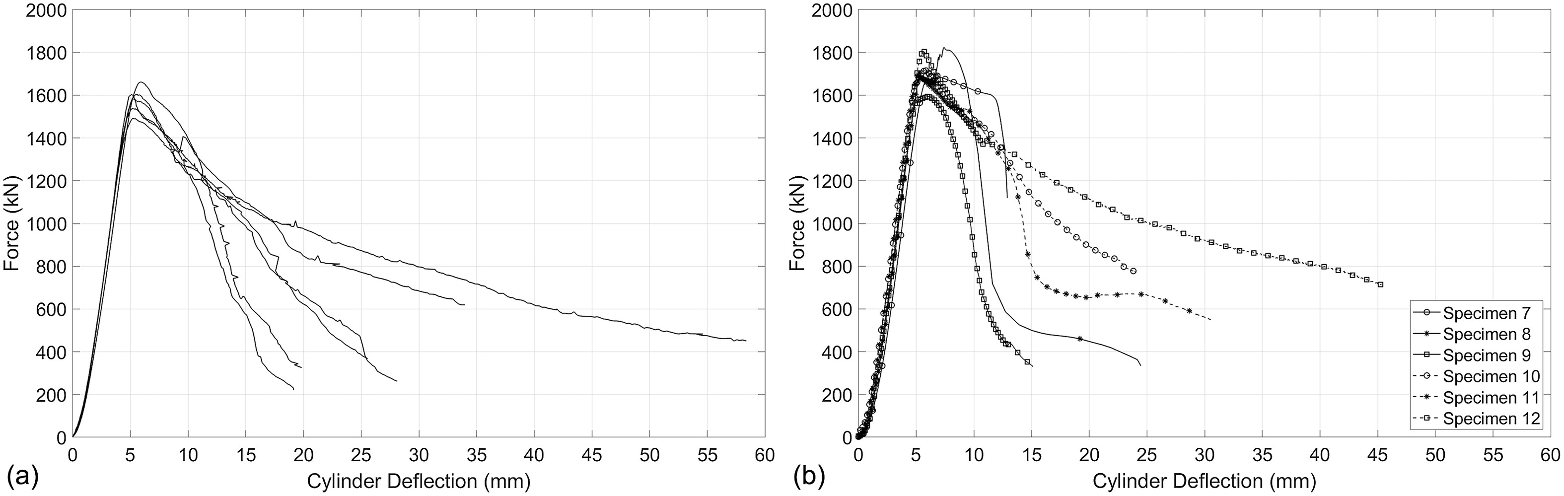
The reinforcement treatments affected the post-peak behavior. Fig. 5 the load-deflection diagram of all the tests. Fig. 5(a) shows the load-displacement curves for the six type A specimens, while Fig. 5(b) presents the load-deflection curve of the type B and type C specimens. As seen from Fig. 5(b) the reinforcement treatments increase the load at failure point. The stress and strain observed in all specimens at 80% of the peak load (i.e., failure point) are presented in Table 3. While there was no significant difference in the strains observed at the failure point, the mean failure stress of type B and type C specimens increased by 8.75% and 11.39%, respectively. Hence, the reinforcement treatment provided by the U-section metal plates increased the loading capacity as compared to the panels with no treatment or with STS only, due to the additive effect from the metal plates, which provide local confinement to the wood fibers. It is to be noted that the U-section metal plates only contributes to the confinement effects of the CLT panel and by virtue of not being continuous from end-to-end, does not directly carry the compressive forces. When using type C reinforcements for CLT panel toe in a rocking wall application, the gross MOE value of these panels is used ignoring any added compressional contact area provided by the U-section metal plates.
| Treatment type | No. | Peak stress (MPa) | Strain at peak stress | Damage onset | Post peak 90% stiffness | 80% of peak stress | ||||||
|---|---|---|---|---|---|---|---|---|---|---|---|---|
| DIC estimation | Visual estimation | |||||||||||
| Stress (MPa) | Strain | Stress (MPa) | Strain | Stress (MPa) | Strain | Stress (MPa) | Deflection (mm) | Strain | ||||
| Type A | 1 | 20.65 | 0.00320 | 10.49 | 0.0013 | 19.32 | 0.0028 | 7.07 | 0.0009 | 16.49 | 10.7 | 0.00630 |
| 2 | 19.73 | 0.00298 | 15.00 | 0.0022 | 19.43 | 0.0033 | 15.17 | 0.0022 | 15.80 | 11.4 | 0.00708 | |
| 3 | 19.94 | 0.00312 | 17.44 | 0.0026 | 19.72 | 0.0034 | 13.38 | 0.0018 | 15.96 | 9.0 | 0.00532 | |
| 4 | 18.54 | 0.00298 | 8.41 | 0.0013 | 16.55 | 0.0026 | 13.86 | 0.0020 | 13.71 | 11.6 | 0.00718 | |
| 5 | 19.16 | 0.00305 | 10.45 | 0.0014 | 15.41 | 0.0023 | 12.01 | 0.0016 | 15.35 | 11.0 | 0.00685 | |
| 6 | 19.95 | 0.00282 | 9.13 | 0.0012 | 19.51 | 0.0028 | 16.56 | 0.0022 | 15.96 | 9.6 | 0.00582 | |
| Mean | 19.66 | 0.00303 | 11.82 | 0.00167 | 18.32 | 0.00287 | 13.01 | 0.00178 | 15.54 | 10.5 | 0.00643 | |
| CoV | 3.70% | 4.35% | 30.33% | 34.42% | 10.13% | 14.58% | 25.37% | 27.57% | 6.25% | 9.82% | 11.65% | |
| Type B | 7 | 21.17 | 0.00320 | 17.24 | 0.0023 | 20.62 | 0.0030 | 16.09 | 0.0028 | 16.76 | 12.2 | 0.00710 |
| 8 | 22.66 | 0.00443 | 17.07 | 0.0025 | 18.98 | 0.0030 | 15.51 | 0.0023 | 18.13 | 9.9 | 0.00613 | |
| 9 | 19.80 | 0.00347 | 12.13 | 0.0017 | 16.37 | 0.0023 | 15.67 | 0.0022 | 15.81 | 8.8 | 0.00527 | |
| Mean | 21.21 | 0.00370 | 15.48 | 0.00217 | 18.65 | 0.00277 | 15.75 | 0.00243 | 16.90 | 10.30 | 0.00617 | |
| CoV | 6.75% | 17.54% | 18.74% | 19.22% | 11.48% | 14.61% | 1.89% | 13.21% | 6.91% | 16.85% | 14.87% | |
| Type C | 10 | 21.33 | 0.00323 | 15.91 | 0.0020 | 21.23 | 0.0036 | 14.07 | 0.0018 | 17.06 | 12.1 | 0.00733 |
| 11 | 21.18 | 0.00277 | 12.89 | 0.0014 | 18.74 | 0.0023 | 16.20 | 0.0019 | 16.93 | 11.6 | 0.00697 | |
| 12 | 22.41 | 0.00283 | 12.07 | 0.0013 | 18.27 | 0.0021 | 15.37 | 0.0017 | 17.93 | 9.9 | 0.00563 | |
| Mean | 21.64 | 0.00294 | 13.62 | 0.00157 | 19.41 | 0.00267 | 15.21 | 0.00180 | 17.31 | 11.18 | 0.00664 | |
| CoV | 3.12% | 8.57% | 14.86% | 24.17% | 8.19% | 30.54% | 7.06% | 5.56% | 3.13% | 10.13% | 13.46% | |
Note: Bold values indicate mean and COV of the group.
Table 2 also presents the load and corresponding displacement values at which the first onset of buckling occurs, as well as delamination or separation of the fiber reaches 25.4mm (i.e., 1 inch). These observations were made after visual assessment of pictures and videos recorded during testing, DIC analysis, and corroborating those with testing notes. Results indicate that when comparing to Type A specimens, the specimens with treatments tend to reach the onset of buckling at lower loads and smaller displacements for the type B specimens and lower loads yet larger displacement for the type C specimens. Moreover, the buckling damage was observed before the failure point on type A and Type B specimens was reached, while for the type C specimens, buckling of the outer lamellas was only observed for strains larger than the ones corresponding to the failure point on type C specimens. Conversely, 25.4 mm delamination damage was observed on all specimens after the failure point. However, these observations could not be statistically confirmed because of the limited number of tested specimens and large CoV observed in the testing results.
Failure Observations
Fig. 6 shows an example of DIC strain maps at three loading levels for a type C specimen. At higher loads, patches of higher strain start to develop around the STS screws. Around 1,350 kN [Fig. 6(c)], prominent strain accumulation is observed around the STS screws.
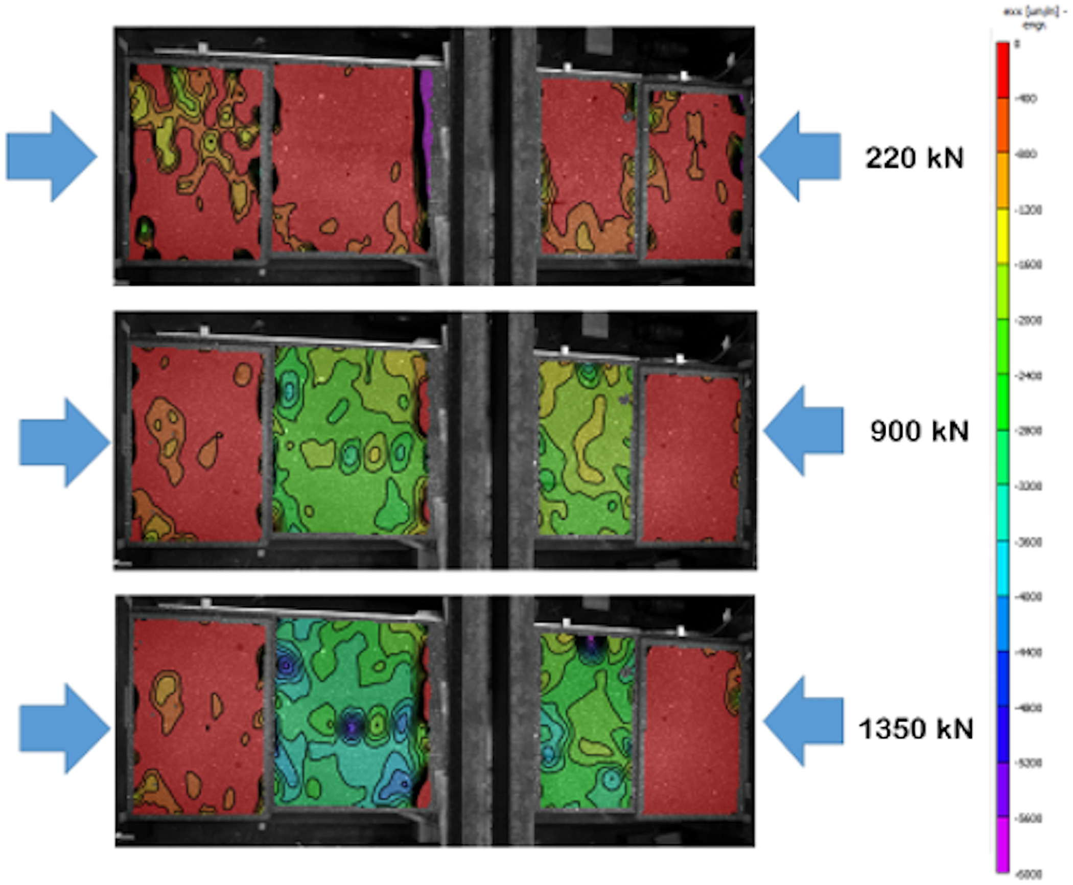
Fig. 7 presents a typical observation from DIC and LVDT data for specimens (for example, specimen 1 in this case) up to assumed failure point. The east and west curves represent the stress–strain curves obtained from W-LVDT1 and E-LVDT1, respectively. The damage points presented in Fig. 7 are the mean of results determined from both east and west curves. The points corresponding to buckling and 25.4 mm delamination damages are not presented in the stress–strain curves. The maximum stress in the specimen was 20.65 MPa corresponding to a compressive strain of 0.0032.
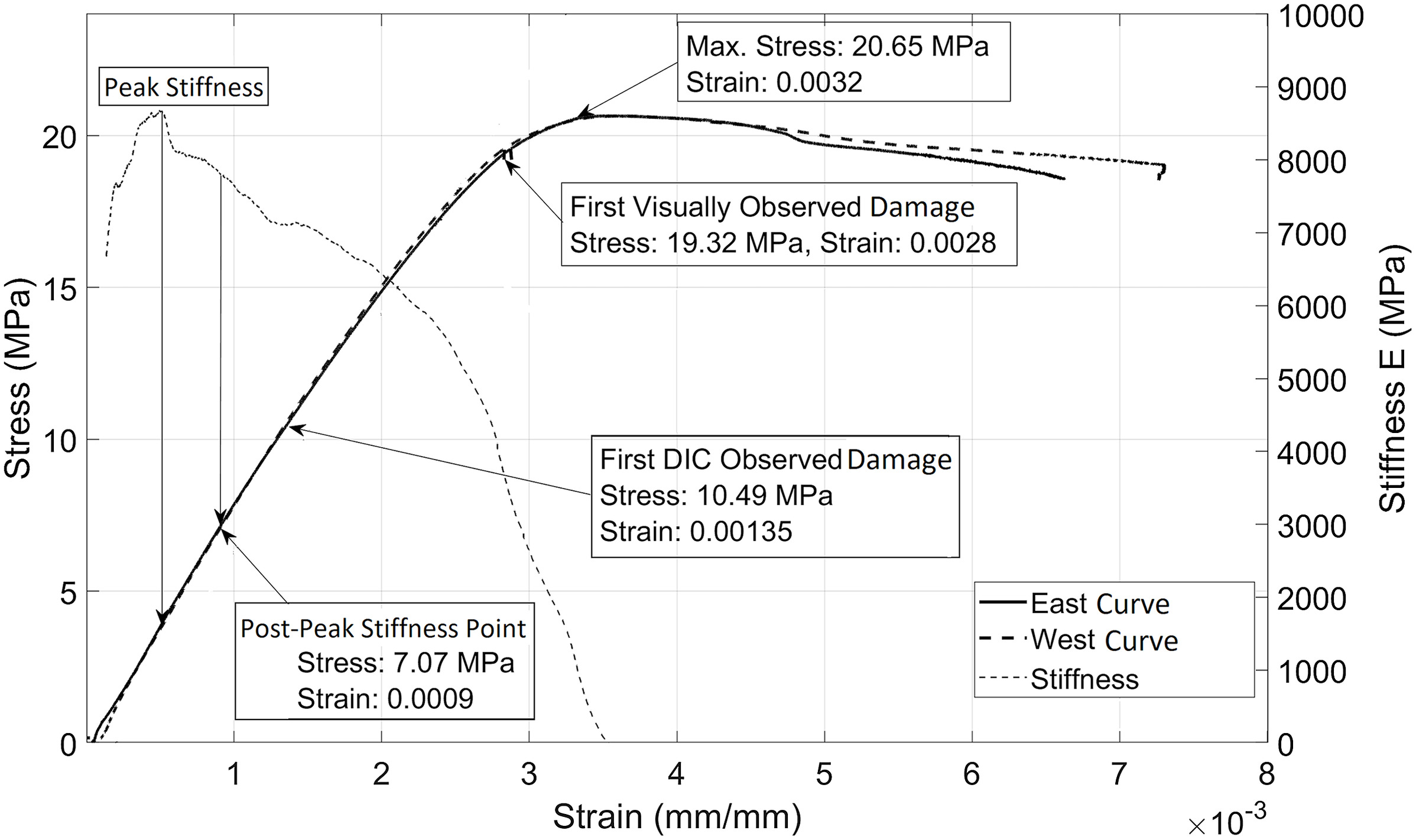
The instantaneous stiffness of the specimen derived from the east curve is shown as stiffness curve in Fig. 7. The stiffness reached its peak at a very low strain of around 0.00051, and a corresponding stress of 3.85 MPa, then quickly decreased. At a stress level of 7.07 MPa, the stiffness was 90% of the peak stiffness value. This post-peak point was defined in this study as an onset of damage in terms of stiffness.
Moreover, from observing the DIC strain map, on specimen 1 the local surface damage started when the stress was 10.49 MPa. At that point, the strain from LVDT data was 0.001346, while the average strain observed from DIC was 0.001232. It is worth noting that the strain map from DIC was for the surface of specimen, so the local damage might have started earlier than the instant in which it was observed based on the strain map. In other words, the observed surface localized damage could be a consequence of a damage inside the specimen, which could not be detected by using DIC. Furthermore, the buckling restraint caused a discontinuity in the speckle pattern and it influenced the field of view for one of the cameras near the edge. As a result, the DIC system was not able to provide meaningful convergence near those edges as evident by the dark and abnormal color contour at the edge of the restraint.
From the correlation of visual observation and the stress–strain curve, the first visual damage was recorded at a stress level of 19.32 MPa and the strain of 0.0028. This failure point is very late compared to the DIC observed onset of failure in stiffness and local damage, but very close to the peak stress point. This observation indicates that the onset of damage determined by visual estimation is not a reliable data point. Fig. 7 also shows the failure point for specimen 1, where the deflection was 10.7 mm corresponding to an engineering strain of 0.0070 at the failure point.
Table 3 presents the results of observations (stress and strain) using the failure estimation methods. Results indicate that the DIC tends to provide a lower bound for the onset of damage stresses and the corresponding strain when compared to those obtained from visual observations, while the visual estimation provides an upper bound. DIC technique observes the displacements of points on specimen’s surface in all three axes and therefore, accounts for out-of-plane deformations within its calculations resulting in earlier detection of the onset of damage vis-à-vis visual estimation as evident in Table 3. The stress at the onset of damage from the visual estimation is very close to the peak stress among all three specimen groups.
There are, however, a few limitations in the instrumentation and data analysis performed. First, a major limitation of DIC is that it only provides surface maps and the state of the material inside specimen is subject to assumptions and interpretations. Therefore, the observed surface local damage could be a consequence of a damage inside the specimen, which could not be detected using DIC. Second, the definition of onset of failure that DIC uses is user dependent and subjective, and if altered will provide different result.
Effects of Confinement
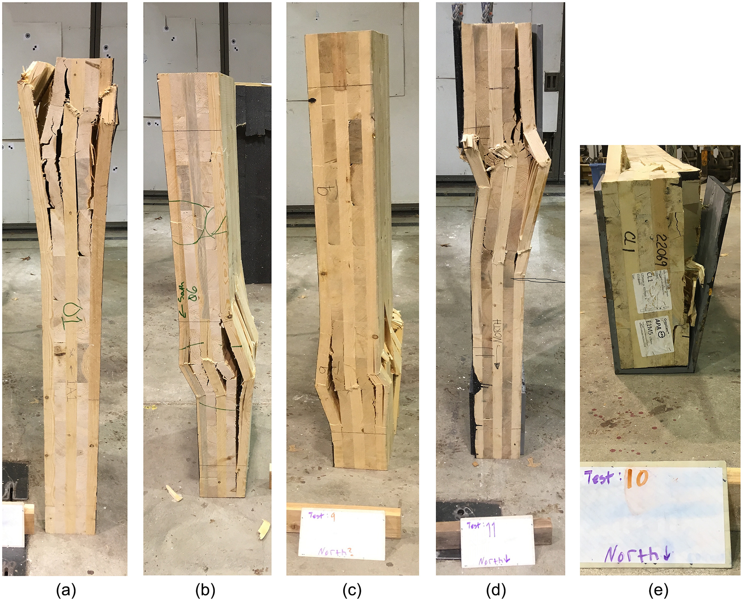
The reinforcement treatments provided some confinement to the panels and thus altered the failure progression of the CLT panels. The specimen without any treatment (type A) failed at random locations along the length of the panel, i.e., the locations at which the specimens failed was not repeatable. Since buckling was restrained, failure was mainly due to excessive crushing, which ultimately led to splitting of the fibers (or delamination) [Figs. 8(a and b)]. The failure at random locations along the length was absent in the specimens with treatments. The samples with only STS screws (type B) also showed localized buckling failures [Fig. 8(c)]. The location of the visible failure was either at the ends where the CLT panel was in contact with the steel loading plate or right below the buckling restraint. The treatment with STS and steel U-channels forced the failure to occur near or within the U-channels [Fig. 8(d)]. The failure was due to crushing and localized buckling of the wood fibers. Past the failure point, the CLT lumber continued to buckle as the test progressed and in-turn expanded the steel U-channels as shown in Fig. 8(e), which was possible as the U-channels were unrestrained from one edge. There was no damage in the screws connecting the U-channels to the CLT panel.
Axial Compression Stress–Strain Models
Three engineering stress–strain models described in the “Material and Methods” section were utilized to represent the stress–strain response of all three different panel types. The input for these stress–strain models and their model parameters are presented in Tables 4 and 5. The numerical model results for three panel types are shown in Fig. 9. The linear function for hardening segment tends to underestimate the stress, while the quadratic function over-predicted the stress in the softening range. Fig. 10 shows a comparison of model II for three panel types and it helps to visually compare the initial slope (i.e., elastic modulus), yield point, ultimate point, and failure point for three panel types presented in Table 4.
| Treatment type | Elastic point | E (MPa) | Ultimate point | Failure point | |||
|---|---|---|---|---|---|---|---|
| (MPa) | (MPa) | (MPa) | |||||
| Type A | 0.00167 | 12.25 | 7,338 | 0.00303 | 19.66 | 0.00643 | 15.54 |
| Type B | 0.00217 | 15.72 | 7,242 | 0.00370 | 21.21 | 0.00617 | 16.90 |
| Type C | 0.00157 | 12.69 | 8,081 | 0.00294 | 21.64 | 0.00664 | 17.31 |
| Treatment type | Function IIa | Function IIb | Function IIIa | Function IIIb | |||||
|---|---|---|---|---|---|---|---|---|---|
| (103) | (109) | (106) | (103) | (103) | (106) | (103) | |||
| Type A | 5.479 | 11.228 | 12.860 | 2.154 | 16.406 | ||||
| Type B | 3.591 | 2.528 | 18.122 | 5.228 | 11.539 | ||||
| Type C | 6.498 | 14.614 | 15.981 | 1.865 | 18.892 | ||||
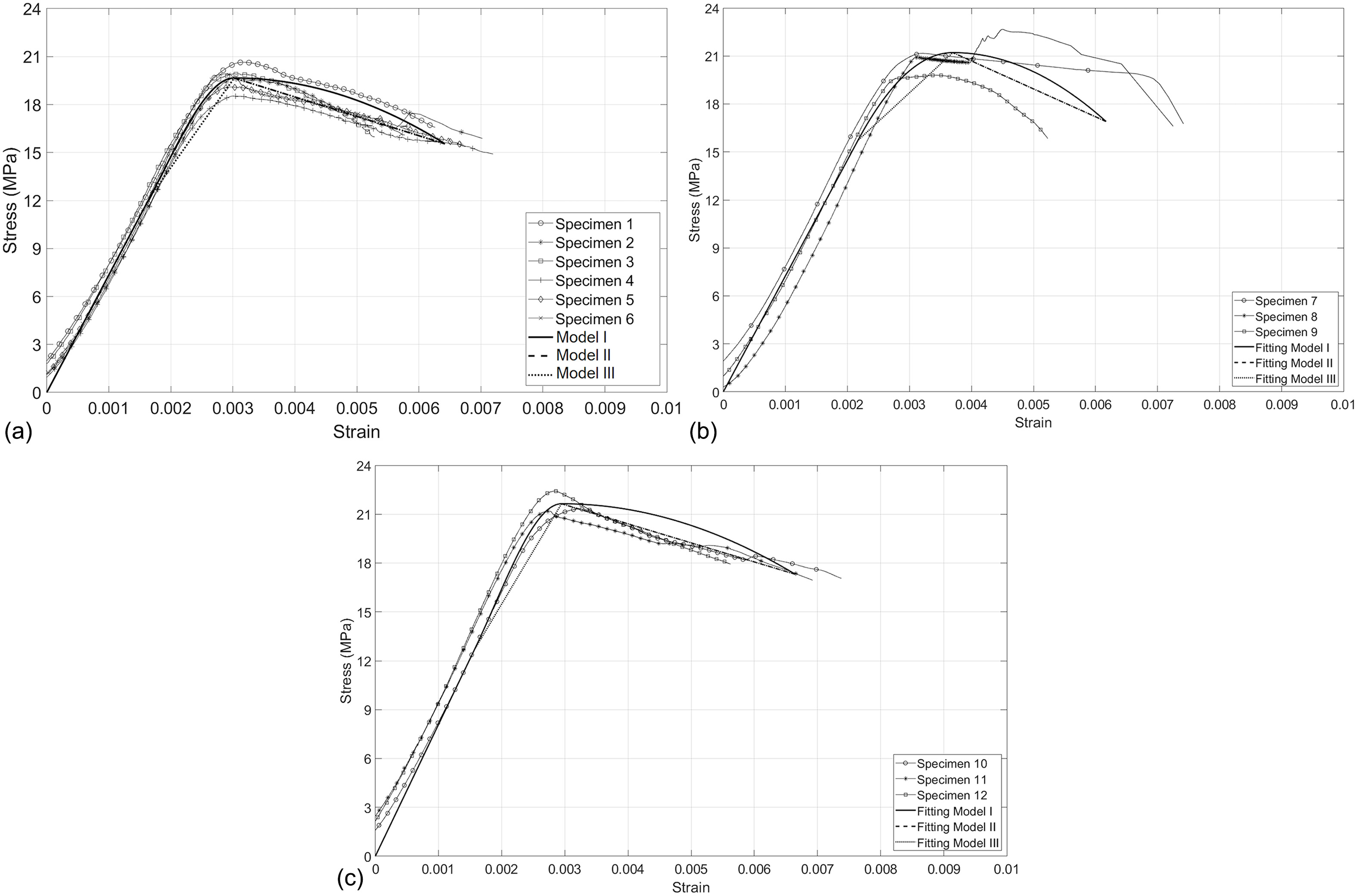
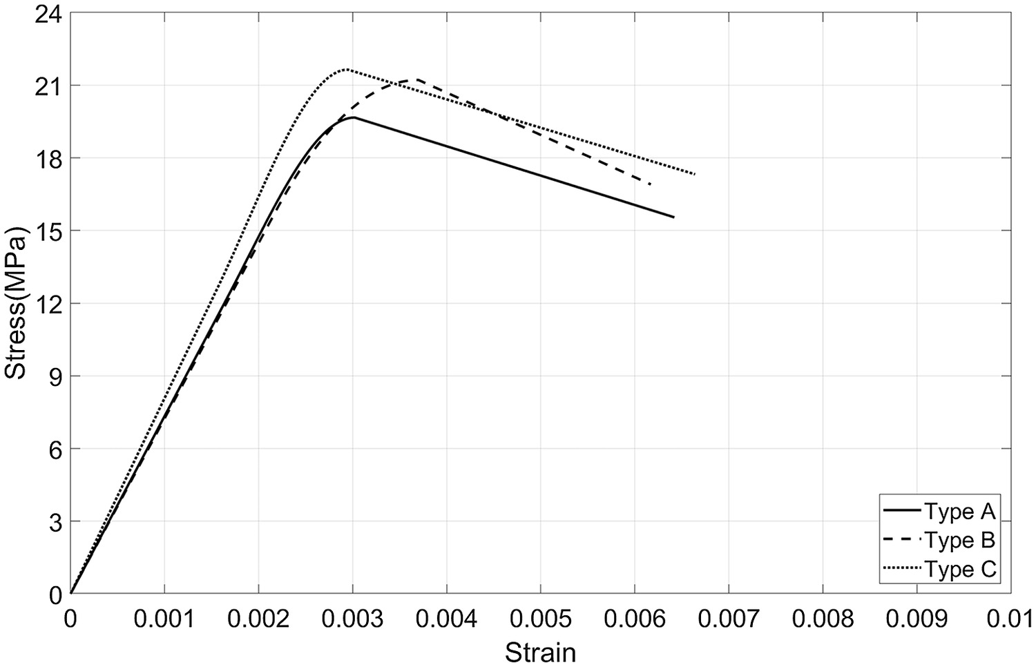
Table 6 provides the results of and for three stress–strain models. Model II, with cubic function for hardening segment and linear function for softening segment, fits best to the experimental data, having resulted in the lowest RMSE and highest values for type A and type B specimens, while model III resulted in the worst fit for all three specimen types.
| Treatment type | RMSE (MPa) | |||||
|---|---|---|---|---|---|---|
| Model I | Model II | Model III | Model I | Model II | Model III | |
| Type A | 0.4555 | 0.3061 | 0.5723 | 0.9939 | 0.9972 | 0.9904 |
| Type B | 0.4298 | 0.5121 | 0.7990 | 0.9959 | 0.9941 | 0.9857 |
| Type C | 1.0625 | 0.7511 | 1.0264 | 0.9667 | 0.9834 | 0.9689 |
Conclusion
A series of tests on large-scale specimens were performed in support of the performance-based seismic design project in the Pacific Northwest in the United States and to improve the understanding of the behavior of mass timber panels under compression. Six bare CLT specimens, three specimens with STS screw reinforcements, and three specimens with STS screws and U-section steel plate reinforcements were tested to characterize the stress–strain behavior of CLT panels under compression up to failure. The onsets of damage, strength degradation, buckling, and 25.4 mm delamination were observed visually and instrumentally by using DIC combined with other instrument results. Results indicate that the engineering values obtained from DIC observations tended to provide a lower bound for onset of damage strains and corresponding stresses, while values obtained from visual inspections provide the upper bound values. Moreover, the tests show that even though both reinforcement types exhibited an increase in the peak load as well as load at failure, the MOE only increased for the type C reinforcement, which is the one that included both STS and U-section steel plates. The treatments also changed the failure progression in the CLT panels, with the failure near the end or right below the buckling restraint, which was due to crushing and localized buckling of wood fibers.
Lastly, three axial compression stress–strain models were developed and calibrated for three specimen types. Model II, with a cubic function defining the hardening segment and a linear function defining the softening segment, fitted best to the experimental data as observed in the and validations.
Data Availability Statement
Raw data were generated as part of this study at Oregon State University. Derived data supporting the findings of this study are available from the corresponding author on request.
Acknowledgments
Financial support for this research was provided by the Framework Project sponsored by the US Tall Wood Building Competition: a partnership between the USDA, Softwood Lumber Board, and the Binational Softwood Lumber Council. In addition, the authors acknowledge the support of the TallWood Design Institute, which subsidized part of the faculty time for this effort. The findings and conclusions of this work are solely those of the authors.
References
Akbas, T., R. Sause, J. M. Ricles, R. Ganey, J. Berman, S. Loftus, D. J. Dolan, S. Pei, J. W. van de Lindt, and H. E. Blomgren. 2017. “Analytical and experimental lateral load response of self-centering posttensioned CLT walls.” J. Struct. Eng. 143 (6): 04017019. https://doi.org/10.1061/(ASCE)ST.1943-541X.0001733.
ANSI/APA (American National Standard). 2019. Standard for performance-rated cross-laminated timber. ANSI/APA PRG 320-2019. Washington, DC: ANSI/APA.
ASTM. 2019a. Standard test methods for cyclic (reversed) load test for shear resistance of vertical elements of the lateral force resisting systems for buildings. ASTM E2126. West Conshohocken, PA: ASTM.
ASTM. 2019b. Standard test methods for cyclic mechanical properties of lumber and wood-based structural material. ASTM D4761. West Conshohocken, PA: ASTM.
ASTM. 2021. Standard specification for high-strength low-alloy columbium-vanadium structural steel. ASTM A572/A572M. West Conshohocken, PA: ASTM.
Blomgren, H. E., S. Pei, Z. Jin, J. Powers, J. D. Dolan, J. W. van de Lindt, A. R. Barbosa, and D. Huang. 2019. “Full-scale shake table testing of cross-laminated timber rocking shear walls with replaceable components.” J. Struct. Eng. 145 (10): 04019115. https://doi.org/10.1061/(ASCE)ST.1943-541X.0002388.
Busch, A., R. B. Zimmerman, S. Pei, R. McDonnell, P. Line, and D. Huang. 2021. “Prescriptive seismic design procedure for post-tensioned mass timber rocking walls.” J. Struct. Eng. 148 (3): 04021289. https://doi.org/10.1061/(ASCE)ST.1943-541X.0003240.
Engleson. 2019. “Testing and modeling of a cross-laminated timber pier-and-spandrel seismic retrofit solution for unreinforced masonry buildings.” Master’s thesis, School of Civil and Construction Engineering, Oregon State Univ.
Framework Portland Project. 2017. “Framework.” Accessed May 1, 2023. https://www.frameworkportland.com.
Ganey, R., J. Berman, T. Akbas, S. Loftus, D. J. Dolan, R. Sause, J. Ricles, S. Pei, J. van de Lindt, and H. E. Blomgren. 2017. “Experimental investigation of self-centering cross-laminated timber walls.” J. Struct. Eng. 143 (10): 04017135. https://doi.org/10.1061/(ASCE)ST.1943-541X.0001877.
Granello, G., A. Palermo, S. Pampanin, S. Pei, and J. W. van de Lindt. 2020. “Pres-Lam buildings: State-of-the-art.” J. Struct. Eng. 146 (6): 04020085. https://doi.org/10.1061/(ASCE)ST.1943-541X.0002603.
Hashemi, A., P. Zarnani, R. Masoudnia, and P. Quenneville. 2017. “Experimental testing of rocking cross-laminated timber walls with resilient slip friction joints.” J. Struct. Eng. 144 (1): 04017180. https://doi.org/10.1061/(ASCE)ST.1943-541X.0001931.
He, M., X. Sun, Z. Li, and W. Feng. 2020. “Bending, shear, and compressive properties of three- and five-layer cross-laminated timber fabricated with black spruce.” J. Wood Sci. 66 (Dec): 1–17. https://doi.org/10.1186/s10086-020-01886-z.
Karacabeyli, E., and B. Douglas. 2013. Cross-laminated timber handbook–US edition. Pointe-Claire, QC: FPInnovations.
MTC Solutions. 2020. Structural screw design guide. Surrey, BC: MTC Solutions.
Mugabo, I., A. R. Barbosa, A. R. Sinha, C. Higgins, M. Riggio, S. Pei, J. W. van de Lindt, and J. W. Berman. 2021. “System identification of UCSD-NHERI shake-table test of two-story structure with cross-laminated timber rocking walls.” J. Struct. Eng. 147 (4): 04021018. https://doi.org/10.1061/(ASCE)ST.1943-541X.0002938.
van de Lindt, J. W., J. Furley, M. O. Amini, S. Pei, G. Tamagnone, A. R. Barbosa, and M. Popovski. 2019. “Experimental seismic behavior of a two-story CLT platform building.” Eng. Struct. 183 (5): 408–422. https://doi.org/10.1016/j.engstruct.2018.12.079.
Wei, P., B. J. Wang, H. Li, L. Wang, S. Peng, and L. Zhang. 2019. “A comparative study of compression behaviors of cross-laminated timber and glue-laminated timber columns.” Constr. Build. Mater. 222 (Oct): 86–95. https://doi.org/10.1016/j.conbuildmat.2019.06.139.
Information & Authors
Information
Published In

Journal of Materials in Civil Engineering
Volume 36 • Issue 8 • August 2024
Copyright
This work is made available under the terms of the Creative Commons Attribution 4.0 International license, https://creativecommons.org/licenses/by/4.0/.
History
Received: May 19, 2023
Accepted: Jan 26, 2024
Published online: May 24, 2024
Published in print: Aug 1, 2024
Discussion open until: Oct 24, 2024
Authors
Metrics & Citations
Metrics
Citations
Download citation
If you have the appropriate software installed, you can download article citation data to the citation manager of your choice. Simply select your manager software from the list below and click Download.