Dynamic Resilience Quantification of Hydropower Infrastructure in Multihazard Environments
Publication: Journal of Infrastructure Systems
Volume 29, Issue 2
Abstract
Ensuring the continued functionality of hydropower infrastructure is of the greatest importance, considering the devastating socioeconomic and environmental impacts of dam operation failures. Among the different approaches currently adopted in hydropower dam operational safety, those that are resilience-based are at the leading edge because they focus on assessing the dynamic system performance pre-, during-, and post-hazard exposures. However, the main challenge for such assessment pertains to the complexity associated with the dynamic operation simulation of hydropower dam systems that consist of several components with nonlinear interdependencies. Moreover, the infrastructure’s exposure to a multihazard environment, which may impact one or more hydropower critical system components, poses further challenges to understanding possible subsequent dam operation failure scenarios. This study develops a resilience-centric system dynamics simulation model that provides a holistic representation of hydropower dam system components to estimate the system’s dynamic resilience in multihazard environments. The study also discusses a combinatorial procedure to generate multihazard scenarios, where a primary hazard can trigger one or more subsequent hazards. Finally, an actual hydropower dam is employed to demonstrate the developed model utility in assessing the resilience of complex infrastructure under a wide range of multihazard scenarios. The proposed model provides valuable decision support tools for infrastructure systemic risk mitigation in multihazard environments—facilitating the development of effective resilience planning strategies.
Introduction
Hydropower dams are critical infrastructure that play a key role to meeting the rapidly increasing global demand for reliable, clean energy (CDA 2019). In addition, hydropower dams are particularly instrumental in water supply management, irrigation, flood risk mitigation, recreation, and river navigation (Branche 2017). However, hydropower dams are also large-scale infrastructure that are highly complex systems of systems—comprised of several intradependent physical (e.g., turbines and gates) and nonphysical (e.g., human decisions, site staff accessing process) components with complex interrelationships. A further complexity of dam behavior predictions pertains to their interdependencies with other dams along the same river system as well as with other critical infrastructure systems, including communications, energy, food and agriculture, transportation, and water (CISA and Homeland Security Department 2015).
Hydropower dams are usually exposed to multihazard environments, where primary hazards—including natural (e.g., floods, earthquakes) and anthropogenic (e.g., lack of gate maintenance, feedback failures) ones—can trigger one or more subsequent hazards. When a dam is exposed to a multihazard environment, the latter may affect one or more of the former system components and subsequently result in an array of different operational failure risks (Hartford et al. 2016). In addition, multihazard environments may rapidly evolve unpredictably during different operational conditions (e.g., inflow discharge), posing further challenges to the dam system operational objectives to meet its performance targets (e.g., fish flow and hydropower demand). Notwithstanding the amplified complexity resulting from simulating the dam system operation in multihazard environments, hydropower dam safety is a critical issue that may have devastating impacts on the environment and the industrial and economic sectors, if not ensured (NPDP 2018).
Considering its importance, various approaches are proposed to develop hydropower dam safety assessment plans, including risk- (Tang et al. 2022; Badr et al. 2021; Zhu et al. 2020; Chen and Lin 2018; Chen et al. 2018), reliability- (Zihui 2020; Zhou 2012; Komey 2014), and vulnerability-based assessments (Nam et al. 2021; Wang et al. 2014; Zhang et al. 2017). Despite the differences between the risk-, vulnerability-, and resilience-based management strategies, all these approaches are essentially risk-informed decision-making tools that are not mutually exclusive. More specifically, vulnerability-based approaches aim to identify the susceptible system components and quantify their tendency to damage or malfunction when a hazard materializes. Risk-based approaches, on the other hand, aim to quantify the potential system functionality losses based on identified system vulnerabilities that would occur during a specific hazard event(s). Finally, resilience-based assessment starts where risk assessment ends by focusing on enhancing the system’s ability to recover more rapidly to a specific target (or original) performance level function of the hazard materializing and the subsequent system performance loss due to specific component vulnerabilities.
Among these approaches, risk-based assessment is the most widely adopted, where the probability of hazard occurrence and the subsequent probability of system failure drive the safety assessment plans (Hariri-Ardebili 2018; ICOLD 2005; Hartford and Bachear 2004). Among the risk quantification approaches, Bayesian networks, along with their different variants including those coupled with Monte Carlo simulations and Markov chain (e.g., El-Awady and Ponnambalam 2021; Badr et al. 2021), showed high efficiency in complex dam systems safety assessment. However, in the past decade, critical infrastructure systems’ safety assessment philosophy has shifted to developing and adopting resilience-based approaches (Lewis 2020). Risk-based assessment focuses more on the immediate response of the system under a specific hazard event (Hosseini et al. 2016; Linkov and Palma-Oliveira 2017; Simonovic 2016). However and as noted earlier, resilience-based assessment focuses more on the dynamic system functionality gain or reduction and, subsequently, the system deterioration and recovery rates following hazard realizations (Baecher 2016). Resilience assessment thus can represent the resource allocations pre- and post-hazard events, as well as restoration costs and recovery time. Furthermore, risk analysis tools (e.g., Bayesian networks) are typically static in nature and may thus not be suitable for simulating the complex (e.g., cyclic and acyclic) system components’ dynamic and feedback relationships. This is the reason it is usually necessary to couple risk analysis tools with other models (e.g., Markov chain, Monte Carlo) to represent the dynamic characteristics of the considered infrastructure system’s operations, which subsequently increases model complexity and computational cost. In addition, most risk analysis tools consider a single value (i.e., probability) to assess the system failure, which does not reflect the evolving changes in the system behaviors that occur during hazard events and its component interdependence.
Alternatively, resilience metrics provide broader insights into the system performance by quantifying system characteristics during and following hazard events (e.g., system’s rapidity, robustness, resourcefulness, and redundancy). Moreover, it is quite challenging to predict complex infrastructure system response and failure modes in a multihazard environment (Little 2010). Accordingly, a sophisticated simulation model is key to providing more meaningful and realistic predictions of the system’s dynamic behavior during and following hazard realizations, to enable its resilience quantification. For further information, the reader can refer to published studies (Guo et al. 2021; Ignjatović et al. 2021; Salem et al. 2020; Lewis 2020; Tong 2019; Linkov and Palma-Oliveira 2017; Baecher 2016; Simonovic and Peck 2013) that discussed the advantages of resilience- versus risk-based performance assessment approaches in developing strategic management plans for complex dynamic systems such as hydropower dams.
Background
System resilience can generally defined as the system ability to bounce back to its normal operating performance level post-hazard disruptions (Salem et al. 2020). Different resilience metrics have been developed since the concept was introduced in the context of ecology by Holling (1973). Hashimoto et al. (1982) proposed the traditional resilience metrics that evolved and were widely adopted in water resources problems and reservoir systems (Kjeldsen and Rosbjerg 2004). However, several studies (e.g., McMahon et al. 2006; Simonovic and Arunkumar 2016) showed the limitations of these static resilience metrics in terms of representing the dynamic nature of dam system functionality disruptions in multihazard environments. As a solution to this time-dimension inconsistency, Bruneau et al. (2003) introduced the four R metrics describing system characteristics following seismic hazard disruption: (1) robustness, describing the system’s capability to maintain the minimum performance level post-hazard occurrence, (2) rapidity, describing the system’s capability to return to the pre-hazard performance level as quickly as possible, (3) redundancy, describing the system capability to provide a backup to substitute the defective component and support the system in regaining its full or partial performance level during the disruption, and (4) resourcefulness, describing the system capability to prioritize necessary recovery resources required for the affected system. By improving the system’s two resilience means (redundancy and resourcefulness), the system may exhibit an enhancement to its two resilience goals (robustness and rapidity). However, most current resilience quantification approaches only consider the system resilience at the end of the simulation period—yielding a single value following only full system recovery. Considering the complexity of critical infrastructure, such a full recovery situation might not be realizable within any practical time frame of interest to decision makers (Ignjatović et al. 2021; Pant et al. 2014). This is because infrastructure managers are typically more concerned with the temporal evolution of their system’s resilience, and subsequently the infrastructure’s critical operational period and times associated with different resilience targets.
As such, Simonovic and Peck (2013) developed a spatiotemporal dynamic resilience quantification approach using system dynamics (SD) (Sterman 2002) to quantify the resilience of coastal megacities under climate-induced hazards. SD modeling represents system components and subsequently estimates their dynamic performance pre-, during-, and post-hazard events and can thus estimate the evolution of system resilience with time. Accordingly, this approach can evaluate, in real time, multiple proactive and reactive adaptation strategies to mitigate the hazard impacts on the exposed system (Simonovic and Arunkumar 2016). Ignjatović et al. (2021) and Simonovic and Arunkumar (2016) showed the advantages of the dynamic quantification approach over the static ones in the context of reservoir systems. However, their developed dynamic resilience quantification approach has key limitations in representing hydropower systems within the focus of the current study. For example, it does not evaluate system resilience in multihazard environments, where a primary hazard can trigger one or more subsequent hazards. This is despite the fact that hydropower dam failures usually occur due to the combinations of natural and anthropogenic hazard events that may be included only individually in the dam’s design envelope (Regan 2010; King et al. 2017; Baecher et al. 2013). In addition, their dynamic resilience quantification approach does not realistically represent the recovery process because it does not consider the practical pre-repair time (repair preparation time taken by the system operators to initiate the repair process and address access logistics, mobilizing services, backup system initiation time), which is a typical feature of complex infrastructure such as hydropower dams (Almufti and Willford 2013, 2014; Choi et al. 2019; Salem et al. 2020). Moreover, their developed SD model was too simplistic and did not include the different dam infrastructure complex system components.
The current study is the first step to developing a dynamic resilience quantification approach for hydropower dam systems in multihazard environments using the SD simulation approach, considering only the deterministic definition for the hazards’ behavior and dam system response. The developed SD model aims to comprehensively represent hydropower dam system components to mimic the multihazard environment’s influence on the performance of the dam system and thus its dynamic resilience. The study also proposes adopting a combinatorial procedure to generate multihazard scenarios, including the natural and anthropogenic ones that may impact the hydropower system performance. Using the estimated dynamic system performance for the generated scenarios, the developed model can quantify the corresponding system resilience evolution with time. Finally, an actual hydropower dam system is considered herein to demonstrate the utility of the developed model in devising a reliable resilience-based assessment for the system operation.
Methodology
Resilience-Centric System Dynamics Dam Model
SD simulation has been shown to be efficient in simulating multiple water resources systems, including hydropower dams (Phan et al. 2021; Winz et al. 2009; Guangze et al. 2021; Lee and Kang 2020; Ahmad and Simonovic 2004). King et al. (2017) provided a general description of using SD in simulating dam system modules (hydraulic, sensors, operation, actuator, and disturbance), including the physical and nonphysical components along with their complex interrelationships. SD can thus provide a comprehensive representation of hydropower components and subsequently estimate system dynamic performance more realistically under various operational conditions. As a result, SD enables the modeler to assess various hazard mitigation strategies in real time, leading to more efficient resilience-based dam operation strategies and safety assessment plans. Following King et al.’s (2017) SD dam modeling approach, the resilience-centric hydropower dam SD model developed herein, shown in Fig. 1, aims to provide a detailed representation of hydropower dam system components and subsequently mimic their system-level performance, which is key for dynamic resilience quantification. As shown in Fig. 1, the SD model integrates six modules, including the four main modules of the hydropower dam system (hydraulic, sensors, operations, and actuators), replicating the dynamic system performance under various operational conditions. The multihazard module is responsible for generating the multihazard scenarios, and, finally, the dynamic resilience module predicts the losses in system performance and the corresponding resilience.

Within the hydropower dam SD model, the hydraulic module represents the variation of the hydraulic variables, including the inflow, reservoir water level, reservoir storage, and outflow releases. The sensor module uses the gauges to record these hydraulic variations and subsequently relay these records to the operation module. Based on the gauge readings and the forecasted hydraulic conditions, the operation module is responsible for determining the instructions to the gates and turbines, considering the dam design operational rules. These instructions are then relayed to the actuator module, including the gates and turbine actuators, to determine the corresponding gate position and powerhouse flow conveyance. The outflow is released according to the gate release and powerhouse flow, considering possible uncontrolled flows such as penstock leakages and overtopping flows. This cyclic operational loop works continuously during normal operational scenarios, where no hazard occurs. However, at the initiation of any hazard scenario, the multihazard module identifies the failed system components associated with a specific hazard. The multihazard module is also responsible for determining the outage time length of the failed components based on the required repair time. Component outage time lengths are typically determined based on the intensity of the hazard impact and the system recovery standards considering all system components. Based on the outage time lengths for different hydropower system components, system performance (i.e., functionality) at each time step can then be estimated by comparing system outputs following hazard exposure and during normal operations (see next section). The dynamic resilience module then employs the estimated system performance to quantify the system’s dynamic resilience (i.e., system resilience values at each time step), according to the quantification approach presented in the next section. Additional details about each module’s components and their interdependencies are presented in the demonstration application discussed in this study.
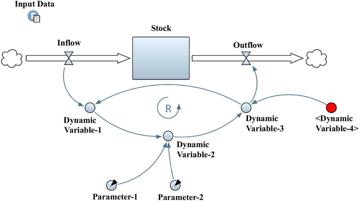
SD is an object-oriented dynamic simulation tool developed based on control theory (Sterman 2002). The SD modeling tool uses the stock-flow representation to represent the whole system architecture, where the stock is represented as boxes and the flows are represented by pipelines that supply (i.e., inflow) or drain (i.e., outflow) the stock, as shown in Fig. 2. These flows change based on the input data (e.g., inflow data series) and also depend on the connected model dynamic variables that represent the system components (e.g., the outflow is determined by the gates and power releases). The connections between the model variables, including flows, parameters, and dynamic variables, are shown as arrows. These connecting arrows reflect the interrelations among the model variables (stocks and nodes). These arrows are defined by mathematical equations or algorithms representing the (static or dynamic) relationships between the connected nodes. The shadow variable, shown between angle brackets (e.g., <Dynamic Variable-4>), represents the relationship between model subsystems (modules). Shadow variables are evaluated by an originating module, and affect other dynamic variables in other connected modules (e.g., the reservoir water level is determined by the hydraulic module, whereas it affects the operation planning variable in the operation module). With the system modules and components and their interrelations defined, input data are imported, and the operational scenarios are generated (normal or exposed-to-hazard scenarios), so SD can simulate the corresponding system’s dynamic behavior and estimate the losses in system performance (in case of hazard occurrence) within the predefined model running time (e.g., 365 days). As such, the presented resilience-centric SD modeling approach can be extended to other critical infrastructure systems considering their system module and component relationships and the expected multihazard scenarios that may affect the system performance. Accordingly, the dynamic resilience quantification approach, explained in the next section, can be adopted to quantify system dynamic resilience corresponding to the generated multihazard scenarios. Readers interested in further description of the SD techniques and their application in water resource research can refer to Phan et al. (2021), Elsawah et al. (2017), and Mirchi et al. (2012).
General Dynamic Resilience Quantification Approach
Dynamic resilience represents the system resilience variation with time, where the system resilience mainly relates to the losses in the system performance due to hazard impact. System performance (e.g., the functionality of the hydropower generation rate, the functionality of gate releases for irrigation or fish flow) refers to the ratio between the actual system’s outputs and the designed system’s outputs that are predefined using the system operational plans according to the system operational targets (e.g., scheduled hydropower rates), as shown in Eq. (1). System performance supposed to be equal unity (i.e., 1.0) during normal operating conditions with no hazard disruptions
(1)
System Performance under a Single Hazard
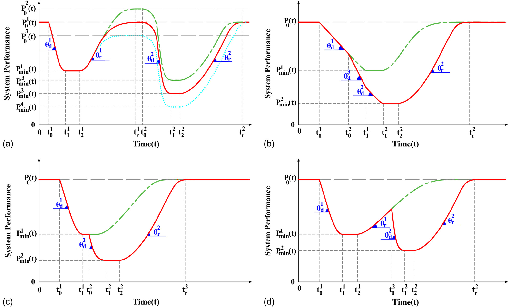
Under hazard exposure, system performance usually deviates from its initial level . Such deviation of the system performance indicates the system performance losses , where represents the area bounded by and during the system’s down period [Fig. 3(a)], starting from (i.e., hazard impact time) until the system bounces back to its target performance level at .

Within the system’s down period ( to ), the system performance typically passes through three different periods. These include the deterioration period representing the deterioration in the system performance while exposed to a hazard, starting at and ending at . Within the deterioration period, deteriorates gradually by a deterioration rate () until it reaches its minimum performance level , indicating the system’s robustness. As the system robustness increases (e.g., through the deployment of risk mitigation plans), the deterioration rate decreases (i.e., ), and subsequently increases [i.e., ], as shown in Fig. 3(b). Moreover, preparedness plans can be deployed to increase system performance prior to hazard impact [i.e., ], so the corresponding to the hazard impact is shifted upward [i.e., ], as shown in Fig. 3(c). As increases, the time needed for the system to return to its target (or original) performance level decreases (i.e., ) and subsequently the system rapidity improves.
The system reaching its triggers the recovery process to restore system performance within the necessary repair time. However, typically, the system first requires a repair preparation time (i.e., pre-repair period) starting at and ending by until the recovery procedure can be initiated (Almufti and Willford 2013, 2014), as shown in Fig. 3(a). The pre-repair period starts at and ends by , including the impeding factors and the utility disruption that delays the start of the recovery process. Impeding factors consider the delay time in initiating the repair and recovery process, which may result, for example, from the requirement of expert inspections, access logistics, and service mobilization. The utility disruption reflects the time required for setting up the tools used in the repair process (e.g., refueling generators, initiation of the backup system). As the pre-repair time decreases (i.e., ), the delay in the recovery process initiation decreases, and subsequently the system recovers faster (i.e., ), as shown in Fig. 3(d).
At the end of the pre-repair time, the recovery period starts at with a recovery rate (), reflecting the system resourcefulness, until it reaches its target performance level at . In the context of hydropower operations, may be higher [i.e., ] or lower than the initial performance level depending on system recovery standards (Simonovic and Arunkumar 2016), as shown in Fig. 3(e). As the recovery rate increases (i.e., ) (e.g., resources are added to accelerate the recovery process), the system recovers faster (Bristow 2019), and system rapidity improves (i.e., decreases), as shown in Fig. 3(f). Fig. 3(g) also shows that enhancing the system redundancy can further improve the system rapidity, where adding a backup system within a period of time (i.e., to ) (e.g., the backup battery can be used in case of dam grid failure) can improve system performance and decrease the recovery period. In the context of hydropower systems, may propagate nonlinearly through the deterioration and recovery processes due to the nonlinear relationships between the system components. The value of is usually smaller than , where may be equal to 90° as the operations may halt essentially immediately when a hazard occurs (e.g., an earthquake may lead to instant tripping or forced outage of the hydropower station).
System Performance in a Multihazard Environment
In multihazard environments, the primary hazard can trigger one or more secondary hazards. Fig. 4 shows a general representation of the system performance under two consecutive hazard events. In Fig. 4(a), the secondary hazard event occurs at time after the system fully recovers from the primary hazard impact at . Each hazard impacts the system with different deterioration rates and may reach different minimum system performance levels . However, the secondary hazard impact may start at different initial performance levels , depending on the target performance level of the primary hazard impact, as shown in Fig. 4(a). As explained previously, the target performance level may be higher or lower than the initial performance level . Accordingly, the corresponding to the secondary hazard impact depends on the system’s initial/normal performance level [e.g., , ]. However, the recovery rates may not change within the two hazard impacts because the recovery rates relate mainly to system resourcefulness and not only to the type or extent of hazard impact. However, the system’s pre-repair time may vary, depending on the hazard type (i.e., to for Hazard 1 and to for Hazard 2). For example, flood events typically cut off roads, increasing the time to access the dam site, subsequently delaying the recovery process. After initiating the system recovery process, bounces back to its target performance level. The target performance under the secondary hazard can be equal to, or larger or smaller than, its initial performance level according to the system recovery strategies to overcome the losses in system outputs (e.g., hydropower energy) that occurred during system downtime. Fig. 4(b) shows the system performance curve , where the secondary hazard occurs during the deterioration period of the primary hazard. As such, the deterioration rate increases during the overlap period starting from to . Subsequently, the system reaches its minimum performance level at the end of the secondary hazard duration, . The pre-repair period is defined based on the secondary hazard type between and . The system starts the recovery process from both hazards at with the recovery rate until it reaches its target performance level at . Fig. 4(c) represents the system performance, where the secondary hazard event impacts the system at during the pre-repair period pertaining to the primary hazard (between and ). The recovery process is delayed until the secondary hazard duration and its re-repair period ends at . Subsequently, the system recovers under the secondary recovery rate until it reaches its target performance level at . Fig. 4(d) shows the system performance, where the secondary hazard impacts the system with the deterioration rate within the recovery period from the primary hazard (i.e., ). The pre-repair time and the subsequent recovery process period are set based on the secondary hazard event.
Overall System Dynamic Resilience Quantification
Using the SD model, the system performance curve and its parameters can be constructed. Subsequently, the system performance losses can be quantified at each time step () by integrating the area bounded between and within the system downtime starting from to , as shown in Eq. (2)
(2)
The dynamic resilience can be calculated at each time step by normalizing the system performance losses over time (Simonovic and Peck 2013), as shown in Eq. (3)
(3)
In the case of two consecutive hazard impacts, where the secondary hazard impacts the systems prior to the system’s full recovery from the primary hazard’s impact [cases represented in Figs. 4(a–c)], both hazard impacts can be assumed as a composite hazard impact that starts at and ends by . As such, Eq. (2) can calculate the system performance losses where should refer to the primary hazard impact time , whereas should refer to the secondary hazard impact recovery time . Subsequently, using the same approach, Eq. (3) can determine the dynamic system resilience by normalizing using and . However, when the secondary hazard impacts the system after the system has fully recovered from the primary hazard impacts, Eq. (2) should consider each hazard impact separately by updating , , and at the beginning of each hazard impact [i.e., , ]. Subsequently, Eq. (3) can be used to calculate the system resilience by updating , , and after the beginning of each hazard impact [i.e., ]. Eqs. (4)–(9) show the and calculations for consecutive multihazards ().
If ()
(4)
(5)
If ( and )
(6)
(7)
If ( and )
(8)
(9)
Using these equations [Eq. (3) for single hazard or Eqs. (4)–(9) for multihazard], dynamic resilience curves can be generated. Fig. 5(b) shows a generic dynamic resilience curve generated using the system performance curve , shown in Fig. 5(a), according to Eqs. (1)–(9) as explained previously. Dynamic resilience curves aim to show the system resilience value evolution pre-, during, and post-hazard impact. The system resilience starts with 1.0 during the normal operation/pre-hazard realization, and then gradually decreases due to the losses in the system performance (i.e., area larger than 0). Such reduction in system resilience depends on the ratio between area , representing the system performance losses , and area , representing the total area as if there is no reduction in system performance. As the system performance losses increase, the system resilience decreases, as shown in Fig. 5(b). System resilience continues its deterioration until it reaches its minimum value at calculated using the total performance losses (i.e., area ) that occurred due to hazard realization. After , the resilience value increases gradually with time , when the system normally operates and no more performance losses occur ( decreases with time as does not exceed , while increases with time). The value of continues to increase until the resilience value converges to approximately 1.0 at , when the system losses are diminished considering the length of time span of system operations (i.e., is much larger than ) under normal conditions. As increases (e.g., , ) or decreases (e.g., , ), this refers to a more resilient system with lower system performance losses occurring due to the hazard impacts. These two metrics ( and ) can be used to assess the efficiency of multiple system operation strategies to mitigate system performance losses due to hazard event impacts.

However, each hazard may have different impacts on the system components (e.g., earthquakes may affect both power and gate releases), and subsequently the overall system resilience must consider all the individual hazard impacts (). Using the previous approach, system performance curves [i.e., ] can be constructed corresponding to each hazard [e.g., ]. Thus, system performance losses and the corresponding dynamic resilience curve per hazard impact can be evaluated using the same approach presented previously (e.g., ). Accordingly, the overall system resilience for all-hazard impacts () can be calculated using the geometric mean as shown in Eq. (10) (Simonovic and Peck 2013). The geometric mean is preferred for quantification due to its efficiency in dealing with outliers and extreme values more than the arithmetic mean, which is very sensitive to outliers (Clark-Carter 2010). In addition, the geometric mean is usually used for calculating rates (e.g., recovery rates) because it considers the compounding that occurs from period to period
(10)
Combinatorial Procedure for Generating Multihazard Scenarios
Multihazard scenario generation is key to quantifying the hydropower system performance as accurately as possible, and subsequently the system’s resilience, using the developed resilience-centric SD model. Multihazard scenarios should consider the possible hazards’ interactions that may impact the considered infrastructure. The hydropower dam system failure may be related to a critical sequence of hazard events that may be individually but not simultaneously included in the dam design envelope (Regan 2010; King et al. 2017; Baecher et al. 2013). Within the hydropower dam system, natural hazards encompass various extreme natural stressors (e.g., earthquakes, floods, wildfires), whereas anthropogenic hazards include several mis-operational and human-made events that affect the performance of system components (e.g., lack of maintenance, delay or erroneous human operational decision, delay site staff mobilization, gates feedback failures).
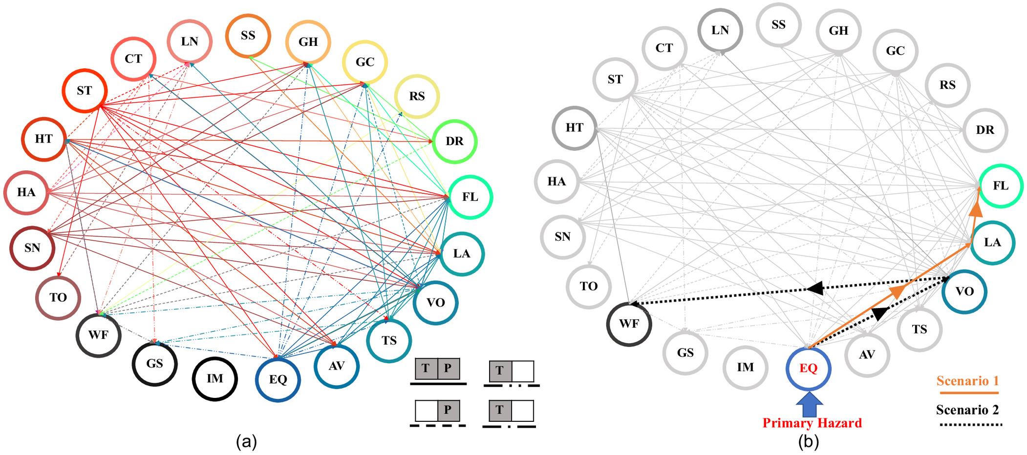
Considering natural hazards interactions, each primary natural hazard may either trigger or increase the possibility of one or more secondary hazard events. These secondary hazards can subsequently trigger or increase one or more hazard events leading to a network effect of interacting hazards. Based on a systematic analysis of several case studies of historical multihazard events, researchers can develop a natural hazards interaction matrix (NHIM) that shows the expected relationships between interacting natural hazards. The current study adopts the NHIM developed by Gill and Malamud (2014) as shown in Fig. 6. The NHIM represents a matrix that identifies 90 natural hazard interactions (out of a possible 441), including both triggering- and increased-probability-of-occurrence relationships.

The 21 hazards are divided into six groups: (1) geophysical hazards, including earthquake (EQ), snow avalanche (AV), tsunami (TS), volcanic eruption (VO), and landslide (LA), (2) hydrological hazards, including floods (FL) and drought (DR), (3) shallow earth processes including regional subsidence (RS), ground collapse (GC), ground heave (GH), and soil subsidence (SS), (4) atmospheric hazards including lightning (LN), extreme cold temperature (CT), wind storm (WS), extreme hot temperature (HT), hailstorm (HA), snowstorm (SN), and tornado (TO), (5) biophysical hazards including wildfire (WF), and (6) space and celestial hazards including geomagnetic storm (GS) and impact events (IM). A detailed description of these natural hazard events can be found elsewhere (Gill and Malamud 2014). The NHIM, shown in Fig. 6, represents the primary hazards on the horizontal rows, and the vertical columns represent the secondary hazards. Each primary hazard can trigger (T) and/or increase the probability (P) of (an) other secondary hazard(s). In addition, each primary hazard event can trigger or increase the probability of a large (dark-gray shading) or only a few (light-gray shading) secondary hazard events. For example, an earthquake event may trigger several landslide events, whereas it may only trigger a single or, at most, a few volcanic eruption events.
Employing the presented NHIM, multi-natural hazards scenarios can be generated. Once the primary hazard is identified, the subsequent secondary hazard events can be predicted using the relationships between the natural hazard events presented in Fig. 6. The spatiotemporal relationships (governing the location and time of occurrence of secondary hazards), as well as intensity relationship (governing the magnitude and the number of possible secondary hazards) between the secondary hazards and the primary hazard, should be considered as detailed in Gill and Malamud (2014). Through such relationships, the conditional probabilities can be quantified and used to relate the primary hazards with their subsequent secondary events within all generated multihazard scenarios. Because the associated uncertainty is out of this study’s scope, the demonstration example presented in this study adopts only the deterministic combination for all the possible scenarios that can be generated using the relationships between the natural hazards presented in Fig. 6—assuming that the probability of the secondary hazard occurrence is equal to 1.0 in each scenario. Fig. 7 represents the procedure of generating the multihazard scenarios using the relationships between the natural hazard events presented in Fig. 6. Fig. 7 shows an example of two multinatural hazard scenarios where the primary hazard is assumed to be an earthquake event. Such an earthquake may trigger landslides or volcano events, as shown in Fig. 6. Subsequently, two scenarios are generated, as shown in Fig. 7, to consider the two possibilities. Scenario 1 simulates the earthquake as a primary hazard that can lead to landslide events that may cause flood events, whereas Scenario 2 simulates the earthquake as a primary hazard that can lead to the volcano event, which can cause wildfires. In both scenarios (and all the generated multihazard scenarios used in the simulations of this study), the probability of occurrence of the secondary hazard (e.g., landslides and floods in Scenario 1, volcanos and wildfires in Scenario 2) is assumed to be equal 1.0.
Unlike natural hazards, anthropogenic hazards have no specific interaction forms or a clearly identifiable interdependence both among themselves or with the natural hazards (e.g., there is no relationship between human delays decision and gate maintenance processes, and similarly there is no relationship between feedback failures and earthquake event occurrences). As such, the full range of the potential anthropogenic hazards is adopted herein to generate all possible combinations of the anthropogenic hazards affecting the status of hydropower dam system components. For example, turbine hoist is tested in maintenance or normal operation status. The anthropogenic hazard scenarios are generated, where each scenario may result in one or more failures of each dam component. For example, the system is simulated where the turbine generator is assumed to be in maintenance, the gates’ operation status is normal, with the presence of debris accumulations that reduces the gate capacities.
By generating the full range of the potential anthropogenic hazards of each component, the generated multianthropogenic hazard scenarios are combined with the generated multinatural hazard scenarios using the all-possible-combinations approach. For example, suppose the hydropower system is exposed to an earthquake followed by a flood hazard during the operational period. This multinatural hazard scenario is simulated with the gates being in maintenance status, while the turbine generator is normally operated, and there are two delay days in the site staff mobilization process. Following this approach, the quantification of the dynamic resilience becomes more realistic and representative of all possible multihazard scenarios that can affect hydropower dam system performance. All the multihazard scenarios (), generated using the all-possible-combinations approach are considered equally likely in dam simulations, where the resilience-centric SD model estimates the corresponding system dynamic resilience curve for each multihazard scenario, considering the probability of occurrence of each scenario is equal to 1.0. Also, this section aims to provide a framework to generate multihazard scenarios for the dynamic resilience quantification; however, other procedures related to any specific infrastructure system design requirements need to be applied to provide the most critical multihazards scenario(s) to be considered for the system safety design.
Methodology Application Demonstration
To demonstrate the utility of the developed methodology, the Cheakamus, British Columbia, Canada, hydropower dam system is considered hereafter. The developed methodology can be deployed on other critical infrastructures by simulating their system component interdependencies and the expected multihazard impacts.
Overview of the Hydropower Dam System
Cheakamus hydropower infrastructure is operated by BC Hydro and is located 30 km from the city of Squamish, British Columbia, Canada. The Cheakamus hydropower system consists of an earth-fill section, overflow wing, saddle dams, and main concrete gravity dam known as the Daisy Lake dam. The Daisy Lake dam is constructed on the Cheakamus River and is connected to the Cheakamus hydropower generating station by a power tunnel with two penstocks at its end to carry the power discharge to the powerhouse that discharges into the Squamish River. Daisy Lake (i.e., the dam’s reservoir) has a live storage of and an average daily inflow of . The normal range of the reservoir water levels is 364.90 m [minimum normal reservoir level (MNRL)] and 377.25 m [maximum normal reservoir level (MaNRL)]. Daisy Lake dam contains two spillway gates with discharge capacity at the maximum reservoir level (MaRL) (378.26 m). The Cheakamus hydropower dam can generate up to 157 MW, corresponding to the maximum power discharge of . All the required dam data, including spillway gate rating curve, stage–storage curve, fish flow (i.e., minimum outflow discharge), and reservoir water level limits, are adopted from BC Hydro (2002, 2005) and King (2020).
Hydropower Dam System Dynamics Model
As per the developed methodology, the resilience-centric Cheakamus dam model integrates six modules, including hydraulic, sensors, operation, actuator, multihazard, and dynamic resilience, as shown in Fig. 8. The hydraulic module represents the dynamic change of the hydrologic and hydraulic variables (e.g., inflow, reservoir water level, reservoir storage, and outflow releases), taking into consideration any overtopping or leak flows. The sensor module subsequently represents the process of recording and transmitting such variation to the operation module. Accordingly, the operation module determines the instructions to the gates and turbine actuator, considering the designed operational rules and the dam’s expected and current hydraulic status. These instructions are then applied by the gates and turbine actuators in terms of adjusting the gate position and the powerhouse flow release. According to the new gate position and powerhouse flow releases, the outflow can be determined by the hydraulic module. Such a cyclic loop operates continuously under normal operational conditions. In case of hazard occurrence, the multihazard module is responsible for estimating the required recovery time for the failed system components corresponding to each hazard impact. According to the total recovery time for the failed system components, the dynamic resilience module can estimate the variation of the system performance with time during and after hazard events. In this example, system performance is measured regarding the power flow and gate spill releases, which can reflect the safety of the dam operations to provide the hydropower generation, fish flow, and irrigation demands under multihazard events. The dynamic resilience module then employs the estimated system performance to quantify the system’s dynamic resilience [, , and ], according to the quantification approach presented previously.

This section represents only a general description of the dam system modules, while the specific details of each module’s components, their interrelationship, and mathematical formulation can be found within Figs. S1 –S7 , Tables S1 –S7 , and Eqs. (S1 )–(S37 ) stated in the paper’s Supplemental Materials. Also, the hydraulic, sensors, operations, and actuator modules are constructed based on the dam SD modeling description stated in King (2020) and King et al. (2017), whereas the multihazard and dynamic resilience module are constructed according to the developed approaches stated previously.
Multihazard Scenario Generations
This section aims to generate the multihazard scenarios used by the Cheakamus SD model required for multihazard dynamic resilience quantification. The multihazard scenarios were generated according to the developed combinatorial procedure using the available Cheakamus dam hazard data in Table 1. The data present each hazard event’s expected range of impact time during the operational year (365 days). In addition, the data present the failed components corresponding to each hazard impact and the average outage time length based on the historical outage data of the Cheakamus hydropower dam. Based on the presented natural and anthropogenic hazard events, multihazard scenarios are generated according to the developed multihazard combinatorial procedure approach. Within the generated scenarios, hazards that impact multiple components (e.g., lightning impact Programmable Logical Controller (PLC)/Remote Terminal Unit (RTU) and/or grid) are considered in all possible scenarios (e.g., Scenario 1 considers lightning impact PLC/RTU component, Scenario 2 considers lightning impact grid, and Scenario 3 considers lightning impact both PLC/RTU and grid). Regarding the hazards with multiple potential impacts on the same component (e.g., earthquake initiates gate failure that may lead the gate to stick in place or collapse), each potential impact is considered in separate scenarios (e.g., in Scenario 1 earthquake leads the gate to stick in place, in Scenario 2 earthquake leads the gate to collapse). Once the multihazard scenarios are generated, the start time of the primary and the secondary hazards are selected based on the expected hazard impact time, listed in Table 1, considering the sequence of the considered hazard events within the scenario. For example, Scenario 1 considers an earthquake followed by lightning events and subsequent debris accumulations. As such, the start time of each of the three hazards is selected considering such sequence of the three hazards and also considering the expected occurrence time on the specific dam considered [earthquake is expected to occur on any day of the year (minimum and maximum ), lightning events usually occur between day 120 and 273, and debris accumulations usually occur between 90 and 334 days]. As the start time of each hazard is selected, prior to the simulation start time, it is fixed and becomes a part of each scenario.
| Hazard type | Hazard | Hazard impact time (days) | Failed component | Component failure description | Average outage time length (days) | |
|---|---|---|---|---|---|---|
| Min | Max | |||||
| Natural hazards | Earthquake | 1 | 365 | PLC/RTU | PLC offline | 6 |
| 1 | 365 | Dam access | Access dangerous | 12 | ||
| 1 | 365 | Penstock | Penstock rupture | 90 | ||
| 1 | 365 | Sensor | No reading | 1 | ||
| 1 | 365 | Gate | Gate failure leads it to remain in place | 7 | ||
| 1 | 365 | Gate | Gate failure leads it to collapse | 240 | ||
| Wind storm | 1 | 365 | Grid | Grid failure | 0.167 | |
| Lightning | 120 | 273 | PLC/RTU | PLC offline | 6 | |
| 120 | 273 | Grid | Grid failure | 0.167 | ||
| Extreme high temperature | 1 | 365 | Sensor | Wrong reading | 25 | |
| Wildfire | 181 | 273 | Grid | Grid failure | 0.167 | |
| 181 | 273 | Dam Access | Access dangerous | 12 | ||
| Snow storm | 1 | 365 | Gate | Gate failure leads it to close | 20 | |
| Anthropogenic hazards | Traffic jam | 1 | 365 | Dam access | Delay access | 12 |
| Voltage fluctuation | 1 | 365 | PLC/RTU | PLC offline | 6 | |
| Lack of maintenance | 1 | 365 | Turbine head cover | Bolt fatigue | 365 | |
| 1 | 365 | Turbine generator | Load rejection | 0.25 | ||
| 1 | 365 | Gate | Gate failure leads it to remain in place | 7 | ||
| 1 | 365 | Sensor | No reading | 1 | ||
| Feedback failure | 1 | 365 | Gate | Gate failure leads it to collapse | 240 | |
| 1 | 365 | Gate | Gate failure leads it to close | 20 | ||
| Debris accumulation | 90 | 334 | Gate | Gate is blocked | 20 | |
| Aging | 1 | 365 | Gate | Gate closes | 20 | |
| Timing (weekend) | 1 | 365 | Site staff | Staff is unavailable | 4 | |
| Timing (evening) | 1 | 365 | Site staff | Staff is unavailable | 1 | |
Source: Data from King (2020).
Analysis Results
The Cheakamus dam SD model was validated with the actual dam outputs, and the SD model outputs constructed by King (2020) under different normal operations using the historical inflow data from 1967 to 1998 adopted from BC Hydro (2002) (see Figs. S8 and S9 stated in the Supplemental Materials). Subsequently, the validated model was used in the dynamic resilience quantification using the generated multihazard scenarios for one of the inflow data series (inflow for the 1998 year was used as it is the most recent inflow data used in the validation).
Dynamic Resilience
This section presents the results of the dynamic resilience nodes for the Cheakamus resilience-centric SD model regarding gate spillway releases, power flow releases, and overall system resilience within the model running time (365 days). According to the generated multihazard scenarios (), the model estimates the system performance losses and subsequently constructs system dynamic resilience curves. Figs. 9–11 show the dynamic resilience curves, within the 365 days, for the multihazard scenarios regarding spillway gate release, power flow releases, and overall system resilience, respectively. To get valuable insights for the decision makers from such a massive number of generated resilience curves ( resilience curves), the figures show the mean and the 90th, 50th, and 10th percentile curves for the estimated resilience values. These curves are not related to uncertainty confidence intervals or tolerance bounds per se; instead, they provide quantitative representations of the resilience curves’ average (i.e., mean resilience curve), highest 10% (i.e., 90th percentile resilience curve), 50% (i.e., 50th percentile resilience curve), and lowest 10% (i.e., 10th percentile resilience curve) values, throughout all simulation time steps. As such, these curves can be useful for decision makers to assess the level of system resilience and can be used to test and compare the effectiveness of multiple resilience-guided assessment strategies (e.g., maintenance or upgrading) to increase system resilience.
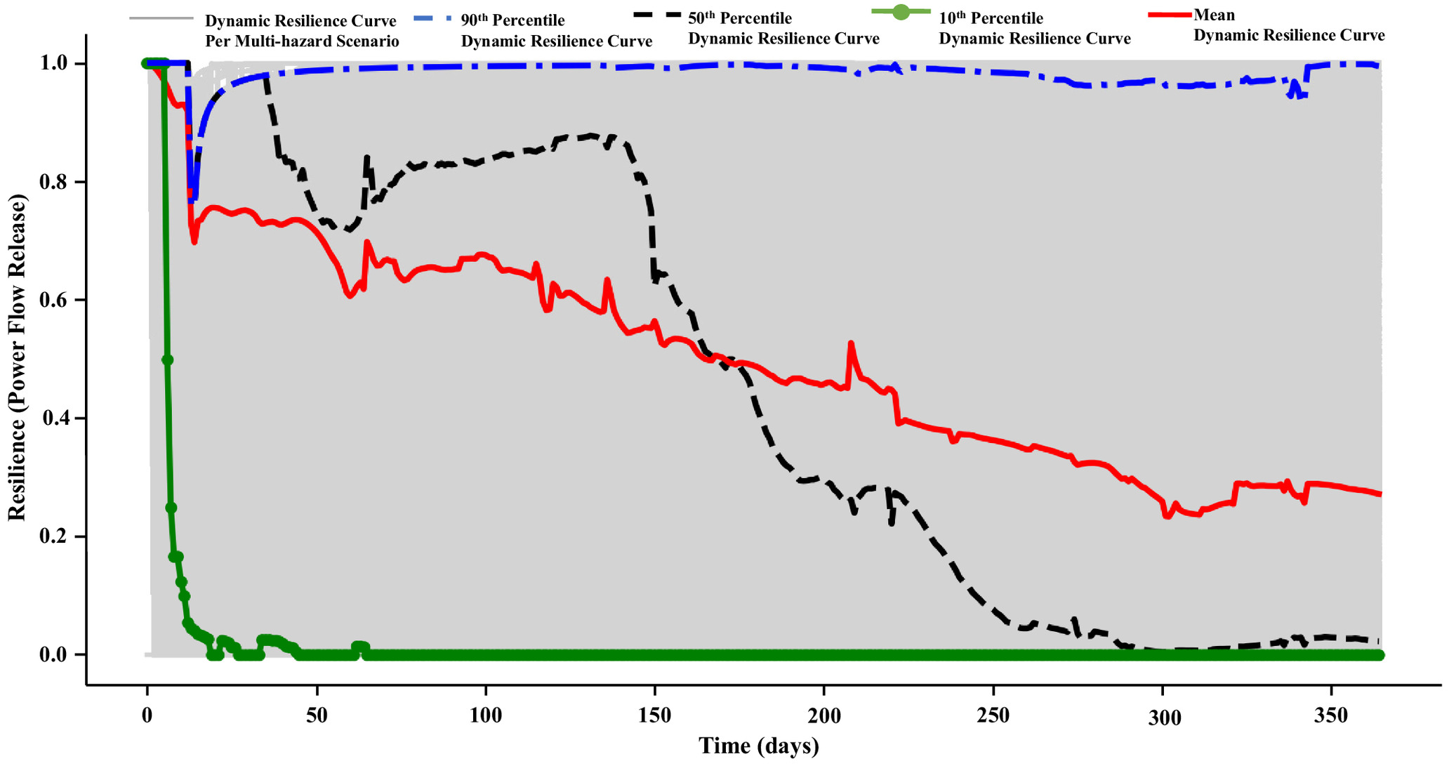

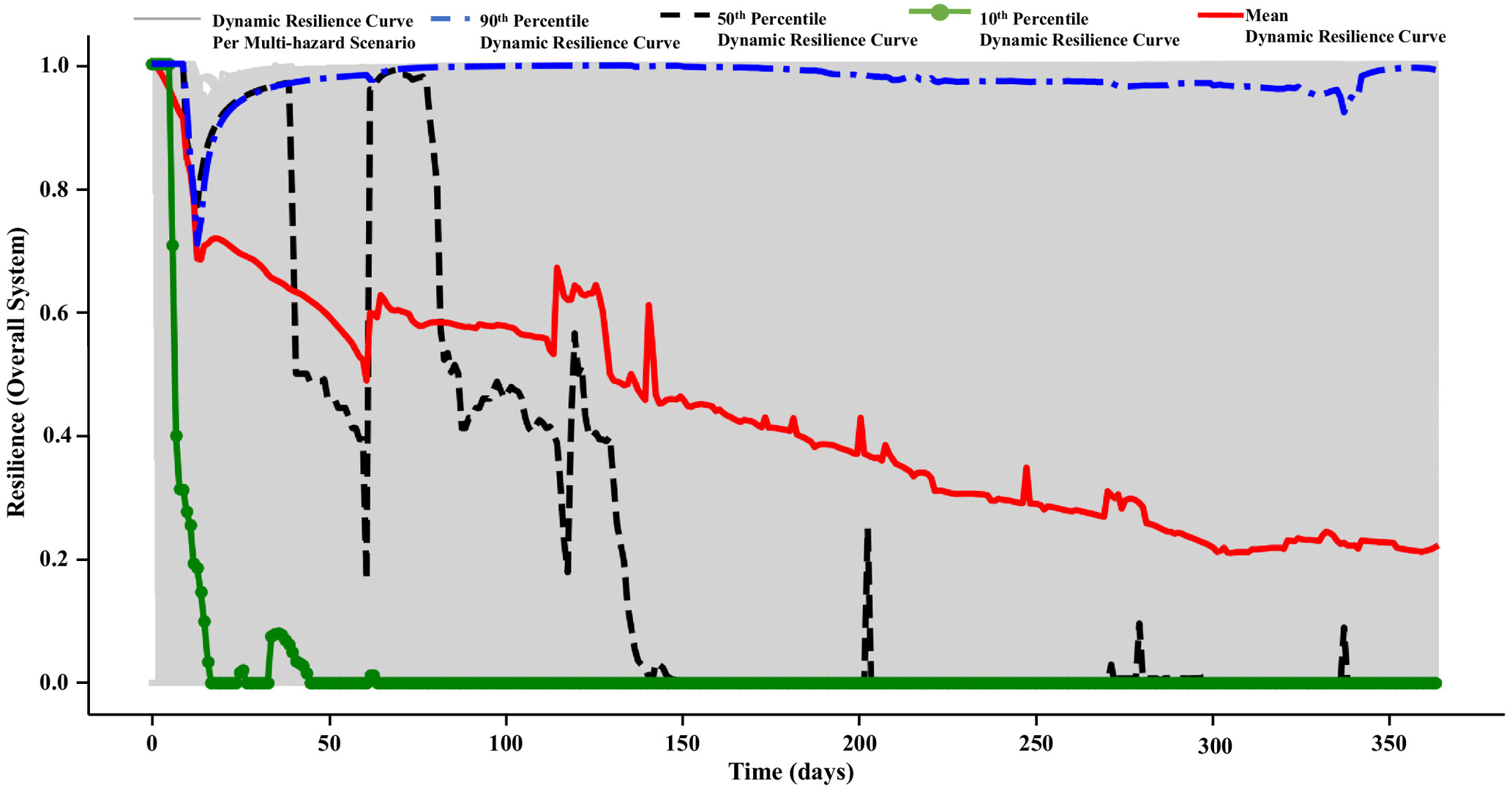
For example, the mean resilience curve in Fig. 11, which shows the average dynamic resilience for the Cheakamus dam system within the scenarios, generally shows a decreasing rate in the resilience values that do not fully return to their standard level within 365 days. The minimum resilience value of the mean resilience curve for the system regarding power release, spillway gate release, and overall system equals 0.234, 0.162, and 0.208, which occurred on 302, 360, and 306 days. The decreasing rate of the mean values refers to the insufficient recovery capabilities of the system to the hazard impacts, where the system does not recover to its standard level within the operational year. For example, the gate collapse and turbine headcover failure require 240 and 365 days on average to recover, which means that if the system is exposed to a hazard that leads to one of the two failures by the first quarter of the year, the system performance is not going to bounce back to its standards within the operational year. Moreover, by comparing the propagation of the mean and 50th percentile resilience curves, the 50th percentile dynamic resilience curve shows a significant drop after 150 days. Such a drop in the 50th percentile value refers to the high frequency of the relatively low resilience values of the system in the second half of the operational year compared with its first half. This can refer to the system’s exposure to more hazards in the year’s second half than in its first half. For example, as given in Table 1, four hazards (lightning, extreme hot temperature, wildfire, and debris accumulation) cannot occur within the operational year’s first quarter. In addition, as the system is exposed to the multihazard environment, and due to the inefficient dam system recovery capabilities, the system may be impacted by the subsequent hazard while it is not fully recovered from the primary hazard impact, which increases the system performance losses and subsequently decreases system resilience values. In this respect, decision makers may consider adding backup systems to join the operation during the expected critical operation periods (e.g., after 150 days in this demonstration example) to hasten system recovery. The 10th percentile resilience curves can also prove relatively high resilience values of the system in the first quarter of the year, where it shows some upward bounces for the resilience values in the three figures within the first quarter of the operational year, although it stays nearly equal to zero until the end of the year.
By comparing Figs. 9 and 10, the system dynamic resilience regarding the spillway gate release is lower than the power flow release. The minimum resilience for the mean and 90th percentile curve for power flow releases is 0.234 and 0.760, while spillway gates’ release mean and 90th percentile value is 0.162 and 0.629, respectively, as given in Table 2. The 50th percentile curves can also show that the resilience of the Cheakamus dam is affected more by spillway gate releases than the power flow releases after 150 days, where the 50th percentile resilience values for the spillway gate release are approximately 0 after 150 days until the end of the 365 days. The relatively lower values of spillway gates release resilience can be explained using Table 1, where 6 of 14 hazards (earthquakes, snowstorm, lack of maintenance, feedback failure, aging, and debris accumulation) directly impact gate components. Besides, the remaining eight hazard events indirectly impact the gate by impacting the dam grid or increasing site staff access time to initiate the manual gate actuation. However, the mean and 50th and 10th percentile dynamic resilience curves for spillway gate releases have relatively higher upward bounces, which refers to the short recovery periods for the spillway gates’ performance compared with the power flow releases’ performance. For example, power flow release performance is affected by the top three failures with long recovery periods, including turbine headcover, penstock rupture, and gate collapses requiring 365, 90, and 240 days, respectively, to recover. Thus, power flow release is affected by a relatively small number of hazards compared with spillway gate release, although such impact takes a relatively long time to recover than the time required for the spillway gate recovery. Table 2 summarizes the minimum resilience value for the mean and 50th, 10th, and 90th percentile curves and the corresponding occurrence time (the corresponding time stated for the 10th percentile refers to the latest time when remained without rebound). Figs. 9–11, according to the study aim, mainly focus on the critical 365-day window, where the multihazard environment occurs, and can provide deep insights into the system behavior within this operational period. However, the time required to show an improvement in the resilience curves is related to each specific scenario, including the normal operation period, the expected number, type, and impact times of the future hazard events, and the corresponding response of the system after the presented 365 days.
| System operational objective | Mean | 90th percentile | 50th percentile | 10th percentile | ||||
|---|---|---|---|---|---|---|---|---|
| Time (days) | Time (days) | Time (days) | Time (days) | |||||
| Power flow release | 0.234 | 302 | 0.760 | 14 | 0.010 | 304 | 0.000 | 64 |
| Spillway gate releases | 0.162 | 360 | 0.629 | 12 | 0.000 | 152 | 0.000 | 99 |
| Overall system | 0.208 | 306 | 0.709 | 13 | 0.000 | 152 | 0.000 | 64 |
Conclusion
This study developed a resilience-centric model for the dynamic resilience quantification of hydropower dam infrastructure in multihazard environments. Using the system dynamics modeling tool, the developed model provides the complex simulation of hydropower dam infrastructure components that is sophisticated enough to mimic the system dynamic performance and estimate the system performance in multihazard environments. The study presents a general dynamic resilience quantification approach applicable to any infrastructure systems under single and multiple hazards. Moreover, the study developed a combinatorial procedure for generating such multihazard scenarios, including the natural and anthropogenic hazards that may impact the system’s performance. Subsequently, the model estimates the corresponding variation of system performance losses and system dynamic resilience under such multihazard scenarios. Presenting the temporal evolution of system resilience can provide decision makers with realistic insights into the infrastructure’s critical operational period and times associated with different resilience targets.
An actual hydropower dam resilience-centric SD model was constructed by integrating six modules, including hydraulic, sensors, operation, actuator, multihazards, and dynamic resilience. The constructed model comprehensively simulates the hydropower system’s physical and nonphysical components and subsequently mimics system performance to generate the dynamic resilience curves under the generated multihazard scenarios. The overall system’s dynamic resilience is calculated by integrating the multihazard impacts on two system components, including the spillway gates and power flow releases performance. The considered hydropower dam system analysis demonstrated the model utility in empowering a resilience-based assessment strategy of the system performance and recovery process in a multihazard environment.
Beyond the current study, the developed modeling approach can further consider different sources of uncertainties, including those associated with the hazard behavior, its occurrence time, frequency, and magnitude, and the corresponding infrastructure system uncertain response and its component interdependencies. In addition, in multihazard environments, the conditional probabilities associated with cascading hazards should also be considered. As a result, uncertainty-induced infrastructure response bands for both the system deterioration and recovery stages, representing probabilistic dynamic resilience, can be generated. Finally, the developed modeling approach can be easily extended to other critical infrastructure considering their system components’ intra- and interdependencies (i.e., with other infrastructure systems) and the potential multihazard scenarios affecting system performance.
Supplemental Materials
File (supplemental_materials_jitse4.iseng-2188_badr.pdf)
- Download
- 818.90 KB
Data Availability Statement
All data, models, and code generated or used during the study appear in the published article.
Acknowledgments
The authors would like to acknowledge the financial support and the fruitful discussions with the research teams of the National Sciences and Engineering Research Council of Canada (NSERC)-the Canadian Nuclear Energy Infrastructure Resilience under Systemic Risk (CaNRisk)-Collaborative Research and Training Experience (CREATE) program, the INTERFACE Institute, and the INViSiONLab. The first author would also like to acknowledge the financial support of his NSERC Vanier Scholarship.
References
Ahmad, S., and S. P. Simonovic. 2004. “Spatial system dynamics: New approach for simulation of water resources systems.” J. Comput. Civ. Eng. 18 (4): 331–340. https://doi.org/10.1061/(ASCE)0887-3801(2004)18:4(331).
Almufti, I., and M. Willford. 2013. REDiTM rating system: Resilience- based earthquake design initiative for the next generation of buildings. San Francisco: Arup. https://doi.org/10.13140/RG.2.2.20267.75043.
Almufti, I., and M. Willford. 2014. “The REDi rating system: A framework to implement resilience-based earthquake design for new buildings.” In Proc., 10th US National Conf. on Earthquake Engineering, Frontiers of Earthquake Engineering, 21–25. Oakland, CA: Earthquake Engineering Research Institute.
Badr, A., A. Yosri, S. Hassini, and W. El-Dakhakhni. 2021. “Coupled continuous-time Markov chain–Bayesian network model for dam failure risk prediction.” J. Infrastruct. Syst. 27 (4): 04021041. https://doi.org/10.1061/(ASCE)IS.1943-555X.0000649.
Baecher, G., R. Ascila, and D. N. D. Hartford. 2013. “Hydropower and dam safety.” Accessed January 23, 2023. http://psas.scripts.mit.edu/home/wp-content/uploads/2013/04/03_Baecher_STAMPWorkshop2013c.pdf.
Baecher, G. B. 2016. “Uncertainty in dam safety risk analysis.” Georisk 10 (2): 92–108. https://doi.org/10.1080/17499518.2015.1102293.
BC Hydro. 2002. Cheakamus River water use plan, report of the consultative committee. Vancouver, BC, Canada: BC Hydro.
BC Hydro. 2005. Cheakamus project water use plan. Vancouver, BC, Canada: BC Hydro.
Branche, E. 2017. “The multipurpose water uses of hydropower reservoir: The SHARE concept.” C. R. Phys. 18 (7–8): 469–478. https://doi.org/10.1016/j.crhy.2017.06.001.
Bristow, D. N. 2019. “How spatial and functional dependencies between operations and infrastructure leads to resilient recovery.” J. Infrastruct. Syst. 25 (2): 04019011. https://doi.org/10.1061/(ASCE)IS.1943-555X.0000490.
Bruneau, M., S. E. Chang, R. T. Eguchi, G. C. Lee, T. D. O’Rourke, A. M. Reinhorn, M. Shinozuka, K. Tierney, W. A. Wallace, and D. Von Winterfeldt. 2003. “A framework to quantitatively assess and enhance the seismic resilience of communities.” Earthquake Spectra 19 (4): 733–752. https://doi.org/10.1193/1.1623497.
CDA (Canadian Dam Association). 2019. “Dams in Canada 2019.” Accessed November 20, 2021. https://www.cda.ca/EN/Publications_Pages/Dams_in_Canada_2019.aspx.
Chen, J., P. A. Zhong, M. L. Wang, F. L. Zhu, X. Y. Wan, and Y. Zhang. 2018. “A risk-based model for real-time flood control operation of a cascade reservoir system under emergency conditions.” Water 10 (2): 167. https://doi.org/10.3390/w10020167.
Chen, Y., and P. Lin. 2018. “Bayesian network of risk assessment for a super-large dam exposed to multiple natural risk sources.” Stochastic Environ. Res. Risk Assess. 33 (Nov): 581–592. https://doi.org/10.1007/s00477-018-1631-0.
Choi, J., N. Naderpajouh, D. J. Yu, and M. Hastak. 2019. “Capacity building for an infrastructure system in case of disaster using the system’s associated social and technical components.” J. Manage. Eng. 35 (4): 04019013. https://doi.org/10.1061/(ASCE)ME.1943-5479.0000697.
CISA (Critical Infrastructure Security Association) and Homeland Security Department. 2015. “Dams sector-specific plan: An annex to the NIPP 2013.” Accessed January 23, 2023. https://www.cisa.gov/sites/default/files/publications/nipp-ssp-dams-2015-508.pdf.
Clark-Carter, D. 2010. “Measures of central tendency.” In International encyclopedia of education. 3rd ed., 264–266. Amsterdam, Netherlands: Elsevier. https://doi.org/10.1016/B978-0-08-044894-7.01343-9.
El-Awady, A., and K. Ponnambalam. 2021. “Integration of simulation and Markov chains to support Bayesian networks for probabilistic failure analysis of complex systems.” Reliab. Eng. Syst. Saf. 211 (Jul): 107511. https://doi.org/10.1016/j.ress.2021.107511.
Elsawah, S., S. A. Pierce, S. H. Hamilton, H. Delden, D. van, Haase, A. Elmahdi, and A. J. Jakeman. 2017. “An overview of the system dynamics processes integrated modeling of socio-ecological systems: Lessons on good modeling practice from five case studies.” Environ. Modell. Software 93 (Aug): 127–145. https://doi.org/10.1016/j.envsoft.2017.03.001.
Gill, J. C., and B. D. Malamud. 2014. “Reviewing and visualizing the interactions of natural hazards.” Rev. Geophys. 52 (4): 680–722. https://doi.org/10.1002/2013RG000445.
Guangze, S., L. Yi, S. Zhang, Y. Xiang, J. Sheng, J. Fu, S. Fu, and M. Liu. 2021. “Risk dynamics modeling of reservoir dam break for safety control in the emergency response process.” Water Supply 21 (3): 1356–1371. https://doi.org/10.2166/ws.2021.004.
Guo, D., M. Shan, and E. K. Owusu. 2021. “Resilience assessment frameworks of critical infrastructures: State-of-the-art review.” Buildings 11 (Jun): 464. https://doi.org/10.3390/buildings11100464.
Hariri-Ardebili, M. 2018. “Risk, reliability, resilience (R3) and beyond in dam engineering: A state-of-the-art review.” Int. J. Disaster Risk Reduct. 31 (Feb): 806–831. https://doi.org/10.1016/j.ijdrr.2018.07.024.
Hartford, D. N. D., and G. Bachear. 2004. Risk and uncertainty in dam safety. London: Thomas Telford. https://doi.org/10.1680/rauids.32705.
Hartford, D. N. D., G. B. Baecher, P. A. Zielinski, R. C. Patev, R. Ascila, and K. Rytters. 2016. Operational safety of dams and reservoirs. London: Institution of Civil Engineers. https://doi.org/10.1680/osdr.61217.
Hashimoto, T. J., R. Stedinger, and D. P. Loucks. 1982. “Reliability, resiliency, and vulnerability criteria for water resource system performance evaluation.” Water Resour. Res. 18 (1): 14–20. https://doi.org/10.1029/WR018i001p00014.
Holling, C. S. 1973. “Resilience and stability of ecological systems.” Annu. Rev. Ecol. Syst. 4 (1): 1–23. https://doi.org/10.1146/annurev.es.04.110173.000245.
Hosseini, S., K. Barker, and J. E. Ramirez-Marquez. 2016. “A review of definitions and measures of system resilience.” Reliab. Eng. Syst. Saf. 145 (Jul): 47–61. https://doi.org/10.1016/j.ress.2015.08.006.
ICOLD (International Commission on Large Dams). 2005. Risk assessment in dam safety management. A reconnaissance of benefits, methods and current applications. Paris: ICOLD.
Ignjatović, L., M. Stojković, D. Ivetić, M. Milašinović, and N. Milivojević. 2021. “Quantifying multi-parameter dynamic resilience for complex reservoir systems using failure simulations: Case study of the Pirot reservoir system.” Water 13 (Jul): 3157. https://doi.org/10.3390/w13223157.
King, L. M. 2020. “Using a systems approach to analyze the operational safety of dams.” Ph.D. thesis, Dept. of Civil and Environmental Engineering, Univ. of Western Ontario. https://ir.lib.uwo.ca/etd/6880.
King, L. M., S. P. Simonovic, and D. N. D. Hartford. 2017. “Using system dynamics simulation for assessment of hydropower system safety.” Water Resour. Res. 53 (8): 7148–7174. https://doi.org/10.1002/2017WR020834.
Kjeldsen, T. R., and D. Rosbjerg. 2004. “Choice of reliability, resilience and vulnerability estimators for risk assessments of water resources systems.” Hydrol. Sci. J. 49 (5): 755–767. https://doi.org/10.1623/hysj.49.5.755.55136.
Komey, A. 2014. “A systems reliability approach to flow control in dam safety risk analysis.” Master of Science thesis, Dept. of Civil and Environmental Engineering, Univ. of Maryland.
Lee, S., and D. Kang. 2020. “Analyzing the effectiveness of a multi-purpose dam using a system dynamics model.” Water 12 (4): 1062. https://doi.org/10.3390/w12041062.
Lewis, T. 2020. Critical infrastructure protection in homeland security: Defending a networked nation. Hoboken, NJ: Wiley.
Linkov, I., and J. Palma-Oliveira. 2017. Resilience and risk; methods and application in environment, cyber and social domains. Dordrecht, Netherlands: Springer. https://doi.org/10.1007/978-94-024-1123-2.
Little, R. G. 2010. “Managing the risk of cascading failure in complex urban infrastructures.” In Disrupted cities when infrastructures fails. 1st ed., edited by S. Graham, 27–39. New York: Routledge.
McMahon, T. A., A. J. Adeloye, and S.-L. Zhou. 2006. “Understanding performance measures of reservoirs.” J. Hydrol. 324 (1–4): 359–382. https://doi.org/10.1016/j.jhydrol.2005.09.030.
Mirchi, A., K. Madani, D. Watkins, and S. Ahmad. 2012. “Synthesis of system dynamics tools for the holistic conceptualization of water resources problems.” Water Resour. Manage. 26 (9): 2421–2442. https://doi.org/10.1007/s11269-012-0024-2.
Nam, M. J., J. Y. Lee, and W. Y. Jung. 2021. “Scenario-based vulnerability assessment of hydroelectric power plant.” J. Korean Soc. Disaster Secur. 14 (1): 9–21. https://doi.org/10.21729/KSDS.2021.14.1.9.
NPDP (National Performance of Dams Program). 2018. “Dam failures in the US.” Accessed January 23, 2023. http://npdp.stanford.edu/sites/default/files/reports/npdp_dam_failure_summary_compilation_v1_2018.pdf.
Pant, R., K. Barker, and C. W. Zobel. 2014. “Static and dynamic metrics of economic resilience for interdependent infrastructure and industry sectors.” Reliab. Eng. Syst. Saf. 125 (Mar): 92–102. https://doi.org/10.1016/j.ress.2013.09.007.
Phan, T., E. Bertone, and R. A. Stewart. 2021. “Critical review of system dynamics modelling applications for water resources planning and management.” Cleaner Environ. Syst. 2 (Jun): 100031. https://doi.org/10.1016/j.cesys.2021.100031.
Regan, P. J. 2010. “Dams as systems—A holistic approach to dam safety.” In Proc., Collaborative Management of Integrated Watersheds, 30th Annual USSD Annual Meeting and Conf., 1307–1340. Denver: United States Society on Dams.
Salem, S., A. Siam, W. El-Dakhakhni, and M. Tait. 2020. “Probabilistic resilience-guided infrastructure risk management.” J. Manage. Eng. 36 (6): 04020073. https://doi.org/10.1061/(ASCE)ME.1943-5479.0000818.
Simonovic, S. P. 2016. “From risk management to quantitative disaster resilience—A paradigm shift.” Int. J. Saf. Secur. Eng. 6 (2): 85–95. https://doi.org/10.2495/SAFE-V6-N2-85-95.
Simonovic, S. P., and R. Arunkumar. 2016. “Comparison of static and dynamic resilience for a multipurpose reservoir operation.” Water Resour. Res. 52 (11): 8630–8649. https://doi.org/10.1002/2016WR019551.
Simonovic, S. P., and A. Peck. 2013. “Dynamic resilience to climate change caused natural disasters in coastal megacities quantification framework.” Br. J. Environ. Clim. Change 3 (3): 378–401. https://doi.org/10.9734/BJECC/2013/2504.
Sterman, J. D. 2002. “Systems dynamics modeling: Tools for learning in a complex world.” IEEE Eng. Manage. Rev. 30 (1): 42. https://doi.org/10.1109/EMR.2002.1022404.
Tang, X., A. Chen, and J. He. 2022. “A modelling approach based on Bayesian networks for dam risk analysis: Integration of machine learning algorithm and domain knowledge.” Int. J. Disaster Risk Reduct. 71 (Mar): 2212–4209. https://doi.org/10.1016/j.ijdrr.2022.102818.
Tong, H. 2019. “A network approach to interdependent infrastructure resilience assessment for natural hazards.” Master’s thesis, Dept. of Civil and Environmental Engineering, Univ. of Western Ontario. https://ir.lib.uwo.ca/etd/6047.
Wang, B., X.-L. Liang, H. Zhang, L. Wang, and Y.-M. Wei. 2014. “Vulnerability of hydropower generation to climate change in China: Results based on grey forecasting model.” Energy Policy 65 (Feb): 701–707. https://doi.org/10.1016/j.enpol.2013.10.002.
Winz, I., G. Brierley, and S. Trowsdale. 2009. “The use of system dynamics simulation in water resources management.” Water Resour. Manage. 23 (7): 1301–1323. https://doi.org/10.1007/s11269-008-9328-7.
Zhang, Y., A. Gu, H. Lu, and W. Wang. 2017. “Hydropower generation vulnerability in the Yangtze River in China under climate change scenarios: Analysis based on the WEAP model.” Sustainability 9 (11): 2085. https://doi.org/10.3390/su9112085.
Zhou, J. 2012. “Reliability-based hydro reservoir operation modeling.” Master of Applied Science thesis, Dept. of Civil, Environmental, and Engineering, Univ. of British Colombia.
Zhu, Y., X. Niu, J. Wang, C. Gu, Q. Sun, B. Li, and L. Huang. 2020. “A risk assessment model for dam combining the probabilistic and the non-probabilistic methods.” Math. Probl. Eng. 2020 (Apr): 12. https://doi.org/10.1155/2020/9518369.
Zihui, M. 2020. “Reliability-based modeling for Missouri River dam system.” Master of Science thesis, Dept. of Civil and Environmental Engineering, Univ. of Maryland.
Information & Authors
Information
Published In

Journal of Infrastructure Systems
Volume 29 • Issue 2 • June 2023
Copyright
This work is made available under the terms of the Creative Commons Attribution 4.0 International license, https://creativecommons.org/licenses/by/4.0/.
History
Received: Apr 21, 2022
Accepted: Dec 3, 2022
Published online: Mar 8, 2023
Published in print: Jun 1, 2023
Discussion open until: Aug 8, 2023
ASCE Technical Topics:
- Analysis (by type)
- Business management
- Dam failures
- Dams
- Decision making
- Decision support systems
- Disaster risk management
- Disasters and hazards
- Dynamic models
- Energy engineering
- Energy sources (by type)
- Engineering fundamentals
- Failure analysis
- Failures (by type)
- Geotechnical engineering
- Hydro power
- Hydrologic models
- Infrastructure
- Infrastructure resilience
- Man-made disasters
- Models (by type)
- Practice and Profession
- Renewable energy
Authors
Metrics & Citations
Metrics
Citations
Download citation
If you have the appropriate software installed, you can download article citation data to the citation manager of your choice. Simply select your manager software from the list below and click Download.