Deep Infiltration Model to Quantify Water Use Efficiency of Center-Pivot Irrigated Alfalfa
Publication: Journal of Irrigation and Drainage Engineering
Volume 150, Issue 5
Abstract
Water shortages in arid regions present challenges in administering water and requires robust water accounting. In southeast Idaho, the Eastern Snake Plain Aquifer (ESPA) supports an important agricultural sector. Due to connectivity between surface and groundwater in the ESPA, quantifying aquifer recharge is also important. Historically, leaching from excess surface irrigation supported incidental recharge to the ESPA, but more efficient irrigation techniques reduced incidental recharge. This paper outlines a deep infiltration (DI) model developed to evaluate infiltration losses from different irrigation practices and soil types. Twelve scenarios were created to simulate an alfalfa growing season under varying climatic and soil conditions. Under some scenarios, modeled infiltration losses increased by 10%–20% coincident with increased application efficiency. The concept of consumptive use efficiency (CUE) is introduced to quantify the proportion of irrigation beneficially used by crops. The model results show that CUE decreased with increasing application efficiency and suggest CUE could be improved 8%–10% for well-drained loamy soils; clay loam soils showed little opportunity for improvement. The results indicate that more efficient irrigation application techniques may increase DI loss if irrigation schedules do not explicitly include soil water storage for the entire rooting zone. These results indicate that in conditions where losses from DI can be reduced, improving water use efficiency depends on precision irrigation scheduling linked to infiltration rates. This model provides a practical method by which infiltration losses from irrigated lands can be estimated. Considering site-specific infiltration would facilitate and prioritize investments meant to improve water use efficiency.
Practical Applications
Irrigation in arid regions usually entails some degree of inefficiency, partly due to water lost through deep percolation. Although some drainage loss occurs under most real-world conditions, it is difficult to measure actual loss. A lack of real information hampers precise estimates and increases uncertainty about actual conveyance and irrigation efficiency. On the other hand, soil infiltration models can utilize existing soil survey maps and guide prioritization and incentives to encourage best practices. This study demonstrates a straightforward application of a soil water drainage model combined with regional soil maps, as could be implemented by water managers. The model was calibrated using observations of crop water use, irrigation application, and soil water content from an irrigated alfalfa field. The calibrated model was then used to describe potential drainage rates from common soil types and weather conditions in southeastern Idaho. The model results indicate that efficient irrigation practices may be best suited to well drained soils, and fewer benefits were observed in poorly drained soils. Even a relatively simple application of this model highlights conditions that are best suited to particular efficiency strategies and help prioritize limited resources for developing best practices for water conservation.
Introduction
Water-limited regions of the world are experiencing increased shortages, driving a need for robust accounting methods in water management. Water shortage in the western US is aggravated by interannual variability of snowpack and flow, declining aquifer levels, and competition for water resources (Konikow 2013; Vano et al. 2010). These arid regions have become the epicenter for sustainable water management goals due to the heavy economic reliance on irrigated agriculture and growing demand in global commodity markets. To support those goals, practical methods are needed to account for the pathways of water movement through the agricultural landscape.
Idaho’s Magic Valley holds some of the most agriculturally productive farmland in the northwestern US. Within the last few decades, attention has been focused on managing the region’s underlying Eastern Snake Plain Aquifer (ESPA), which provides about half the water used to irrigate of farmland (Stewart-Maddox et al. 2018). Since the 1970s, the aquifer levels have declined, largely attributed to increased pumping, population growth, and increased irrigation efficiency (Johnson et al. 1999). Ultimately, reduced spring flows from the ESPA have decreased surface water availability. This has led to a number of legal challenges between Idaho’s surface-water and groundwater rights holders (Olson et al. 2016). In an effort to reduce conflicts between users, long-term funding supports an aquifer recharge program in parts of the Eastern Snake Plain demonstrating high connectivity between surface and groundwater (Miller et al. 2021). Additionally, policymakers have encouraged participation in surface and groundwater coalitions (Kliskey et al. 2019) and provided irrigation subsidies to update aging infrastructure and line canals (IDWR 2024).
Given the region’s unique hydrology and economic importance of the ESPA, estimating the inflows of water to aquifer storage is a critical part of regional water management. As was demonstrated in the ESPA, groundwater recharge from flood irrigation and other inefficient water application methods contribute measurably to aquifer storage (Johnson et al. 1999; Niswonger et al. 2014; Perry 2007). In recent years, the adoption of irrigation technology has been promoted to save water by reducing nonconsumptive use, such as runoff, wind loss, evaporation, and infiltration below the root zone. This is done by increasing the application efficiency (AE) of overhead irrigation systems, where AE is a measure of how well the system delivers water to the root zone (Irmak et al. 2011).
However, it is difficult to quantify how much total water an efficient irrigation system might save with regard to the entire hydrologic system. This is especially true when considering deep infiltration, which occurs when applied water seeps below the depth from which crops can access and extract soil water. When total losses are considered, more efficient systems do not necessarily conserve water or reduce losses (Contor and Taylor 2013; Grafton et al. 2018), and may even lead to increased consumptive use (Perry et al. 2009; Ward and Pulido-Velazquez 2008).
A number of recent studies have directly compared the application efficiency of center-pivot irrigation systems, including midelevation spray application (MESA), low-elevation spray application (LESA), and low-energy precision application (LEPA) spray nozzle packages. Generally, LESA and LEPA systems are reported as reducing water consumption by 10% to 20% under some field and weather conditions (Peters et al. 2016). Rajan et al. (2015) reported finding AE of 60% to 70% for MESA, 70% to 80% AE for LESA, and greater than 90% for LEPA. Molaei et al. (2021) compared the irrigation of mint, finding no decrease in quality or yield with LESA or LEPA systems despite a 15% reduction of applied water. Using stable isotope analysis of soil water irrigated by LESA and MESA systems, Al-Oqaili et al. (2020) found that LESA decreased soil evaporation, in which evaporation accounted for losses ranging from 3% to 21% in LESA systems. Nonetheless, each of these studies cited the difficulty in attributing changes in measured efficiency to a specific loss.
Water that percolates below the effective root zone of the crop is referred to as deep infiltration (DI); other terms used in research and industry include seepage loss, infiltration losses, and deep percolation. Practical challenges to measuring DI necessitate a variety of complementary monitoring and modeling techniques. Several methods to estimate DI were outlined by Gee and Hillel (1988), including lysimeters, tracer tests, soil water balance (SWB) models, and soil water flow models. Šimůnek (2015) used measured soil properties such as tension and hydraulic conductivity. Hunink et al. (2011) covered several existing soil water and crop simulation models, including AquaCrop (Steduto et al. 2009), CropSyst (Stockle et al. 1994), and soil and water assessment tool (SWAT) models (Arnold et al. 2012), where estimated DI is an ancillary result to main model outputs. Arnold (2011) estimated deep infiltration in irrigated agriculture, using an unsaturated zone water-balance and water-table fluctuation approach to model furrow and sprinkler irrigated crops. More recently, Gómez et al. (2022) predicted DI in irrigated and nonirrigated pasture fields in Oregon using SWB and water-table methods. Irrigation intensity on groundwater levels was explored by Lian et al. (2022) using nonparametric statistic and groundwater level measurements in cultivated pasture.
Recently, remote-sensing data have been coupled with SWB models to provide continuous estimates of soil water content and evapotranspiration (ET) (Calera et al. 2017; Ferreira et al. 2022). Remote-sensing models can provide a map of actual ET across an entire land surface, which has helped improve regional soil water balances. For water managers in southeast Idaho, satellite-based ET has been incorporated into the Enhanced Snake Plain Aquifer Model (ESPAM). Deep infiltration from irrigated lands has been estimated for ESPAM by accounting for on-farm soil water balances (Cosgrove et al. 2006). Along with soil water terms and effective precipitation, an ET adjustment factor is used to account for water shortage, crop disease, and method of application. A limitation to this approach is the water balance is limited to an irrigation entity, making it difficult to quantify field-scale management practices.
A practical approach to estimating field-scale DI is the Irrigation Scheduler from Washington State University (Peters et al. 2019). The app uses weather data to estimate ET using the crop coefficient method (Allen et al. 1998), allowing farm managers to schedule irrigation based on local conditions and management practices. The irrigation requirement and DI losses can be visualized graphically using a simplified soil water balance.
Widespread adoption of efficient irrigation systems and growing scarcity of groundwater combine to generate increasing uncertainty about interactions among soil water storage, deep infiltration losses, and groundwater recharge. Simple models can provide order-of-magnitude estimates of water consumption over broad geographic extent without the need for complex parameterization and avoid potentially unrealistic calibrations. These simple model estimates can highlight potential inefficiencies and prioritize research questions for more comprehensive models and field verification. This current study aims to address knowledge gaps related to DI losses under sprinkler irrigated systems with a simple model based on governing equations for soil water movement. This model was implemented with readily available soil characteristics and a field-based calibration. The model builds on existing irrigation scheduling tools by incorporating a root water extraction function that considers plant water stress. The model outputs can be combined with ET data products to implement a practical accounting method for field- or basin-scale water budgets.
The model was initially calibrated using 3 years of sensor data (soil, irrigation, and evapotranspiration) collected at an irrigated alfalfa field. The calibrated model was then adapted to estimate deep infiltration for irrigated alfalfa fields across the Magic Valley, under 12 scenarios spanning a range of climatic and soil conditions typical to the region. Daily irrigation schedules were designed based on common center-pivot system designs used in the region and typical alfalfa cuttings. The modeled results showed an expected range of DI under different field conditions, irrigation practices, and weather patterns. These estimates can be used to generate boundary conditions in more complex hydrologic models typical in water resource management. The DI model is also a useful tool for optimizing on-farm water conservation and evaluating the cost-effectiveness of new irrigation techniques and technology.
Methods
Model Overview
The deep infiltration model tabulates a one-dimensional daily soil water balance that simulates soil water flow in the root zone of an irrigated crop. The downward flux of soil water is modeled using an modified form of the decay function proposed by Ogata and Richards (1957) to solve for soil water storage on a daily time step [Eq. (2)] (Liu et al. 2006). The model simulates soil water flow and calculates a SWB for each layer within the effective root zone; infiltration occurs when a layer exceeds the soil water-holding capacity, which is determined using water content thresholds. These thresholds include field capacity (FC), saturation (SAT), wilting point (WP), and management allowable depletion (MAD) and are commonly used for irrigation scheduling as a simplified estimate of available water content in the root zone of a crop (Veihmeyer and Hendrickson 1931).
As part of the soil drainage equation, the model calculates infiltration when soil water storage exceeds FC on a volumetric basis, where FC is the soil water content after gravitational drainage. Deep infiltration is defined as the drainage from the lowest boundary layer of the model; this layer also defines the effective root zone, or the depth at which most root extraction in the soil profile has occurred. The effective root zone and soil layers can be parameterized for each crop and soil profile characteristics.
Model Functions
Soil water storage (SWS) on day is calculated using the following soil water balance equation:where = total soil water storage in the soil profile of the previous day; = total soil water storage for today; Irr = scheduled irrigation; AE = irrigation application efficiency; DI = deep infiltration from the lowest soil layer; and RWE = root water extraction, which is a function of evaporative potential (i.e., ET). Rainfall occurring during the growing season was ignored from the SWB equation; antecedent soil water storage was used to account for precipitation that largely occurs during winter months in the area of study. The soil profile is represented by layers where the change in soil water storage at layer from the previous day’s soil water storage is given by Ogata and Richards (1957):where = water content value between field capacity and saturation; and = negative value describing hydraulic conductivity (Liu et al. 2006). Infiltration from layer to adjacent lower soil layer ( + 1) is then calculated as the difference between the change in soil water storage and that from the previous daywhere = infiltration. DI is the that drains from the lowest layer.
(1)
(2)
(3)
Process-based functions that simulate root water extraction are given in Table 1. All functions are calculated for each layer separately, although the soil water balance is explicitly shown for each layer to emphasize the sequence of irrigation and infiltration as inputs. Total soil water potential is partially calculated using soil texture characteristic equations, where SWS is related to matric potential using coefficients of moisture-tension (Saxton and Rawls 2006) [Eq. (4)]. The depth of a given soil layer from the soil surface, as well as the gravity constant (), are summed with matric potential to determine total soil water potential for each layer.
| Name | Symbol | Input variables | Equation | Equation number |
|---|---|---|---|---|
| Soil water potential | Matric potential (kPa) | Eq. (4) | ||
| SWS | Soil water storage (mm) | |||
| , | Coefficients of moisture tension | |||
| Plant water stress | Total soil water potential (kPa) | if | Eq. (5) | |
| 33 kPa | then | |||
| 1,500 kPa | if | Eq. (6) | ||
| Potential at MAD (kPa) | then | |||
| Inflection point | if | Eq. (7) | ||
| , | Saturated water stress constants | then | ||
| , | Unsaturated water stress constants | if | Eq. (8) | |
| , | Decay constants | then | ||
| if then | Eq. (9) | |||
| Root mass | , | Linear root mass constants | Eq. (10) | |
| H | Vertical height (m) from soil surface | |||
| Weighted root mass factor (0–1) | ||||
| Root water extraction | Reference ET (mm/day) | Eq. (11) | ||
| ETrF | Reference ET fraction | |||
| Stress factor (0–1) | ||||
| RWE | Root water extraction (mm) |
Plant water stress is the limiting factor on crop ET due to ambient soil water storage and is modeled using piecewise functions based on soil water potential as shown by Eqs. (5)–(9). Water stress factors () range from zero to one, where zero represents a nonrecoverable crop stress and one represents no water stress to the crop. Above saturation and below management allowable depletion, soil water potential is assigned a value piecewise exponential function is used to represent water stress below an inflection point, which was set at for alfalfa.
The final root water extraction calculation [Eq. (11)] includes the daily reference ET () and reference ET fraction (ETrF). refers to the ASCE standardized reference evapotranspiration, which is based on local, daily weather data, and calibrated to a well-watered, full cover alfalfa crop; is used to approximate a theoretical maximum ET rate for ideal growing conditions (Allen et al. 2005). The reference ET fraction is defined in this study as the ratio of actual ET () to , where is the actual quantity of water removed from the surface. ETrF is a term previously used by Allen et al. (2011) to extrapolate estimates of ET for remote-sensing ET models and is comparable to the function of a crop coefficient (Allen et al. 1998). Similarly, this study uses the ETrF as a simplified approach to adjust based on the crop response to atmospheric conditions and cutting events for alfalfa.
Lastly, a root mass function [Eq. (10)] assigns a weighted factor to each layer based on a linear relationship with depth below the soil surface and is normalized by the depth of each layer. The weighted root mass factor is used together with , ETrF, and to determine the depth of soil water extracted from each modeled layer, i.e., the amount of water contributing to total crop ET.
Model Calibration
The infiltration model was calibrated using measured soil water content data from a field of center-pivot irrigated alfalfa. Given the extent of the soil water content data footprint, calibration of modeled SWS was limited to Layer 1. Three years of data (2018–2020) were collected at the field, which is located within the Harney Basin Watershed located 48 km southeast of Burns, Oregon, and receives about 150 mm of annual precipitation. The dominant soil type for the site is the Poujade series, described as well-drained fine sandy loams (Soil Survey Staff, n.d.). Soil texture properties for this series were used to define water content thresholds (i.e., SAT, FC, and WP).
In situ volumetric water content (VWC) and actual evapotranspiration () collected at the field site were used to constrain simulated behavior of SWS in Layer 1 of the root zone. These data aid in setting a realistic boundary of water availability and demand typical for irrigated alfalfa grown in semi-arid climates. CS616 Water Content Reflectometers (Campbell Scientific, Logan, Utah) were installed about 2.5 cm below soil surface; probe rods oriented vertically per manufacturer guidelines are indicative of VWC for the upper 30 cm of soil above the probe (Campbell Scientific 2020).
Raw VWC collected at the site were corrected for sensor drift and outliers based on physically realistic values for these soils. For example, observed VWC readings were above 45% for extended periods of time (30% to 70% of the time series), which is greater than the saturated moisture content for the soil type (USDA 2021). Corrections were made by first calibrating raw VWC using the linear coefficients for sandy loam soils with saturated electrical conductivity of provided in the sensor manual (Campbell Scientific 2020). Using Poujade series soil texture values, water content thresholds were estimated using pedotransfer functions given by Saxton and Rawls (2006), which were used to guide manual corrections for CS616 readings. The final correction was found to decrease the offset by 50%. The offset was applied to all VWC data collected at the site from 2018 to 2020.
As given in Eq. (2), the and constants are soil-specific values used to simulate soil drainage using the decay function. To simulate SWS for irrigated alfalfa grown in the Poujade series, the constant was set at a value between FC and SAT. The possible range of constant values for silt loam soils were parameterized using empirical values from Liu et al. (2006). Liu et al. (2006) gave a general guideline for silt loam constants, where for quick draining soil and for slow draining soils. The range of uncertainty in for model calibration were based on .
Other soil-specific parameters used in model calibration are described in Table 2. These include water content thresholds, soil-tension coefficients to determine matric potential [Eq. (4)], and initial SWS on day for three soil layers. For Soil layer 1, the initial SWS was based on VWC content on day for the observed soil moisture data. For model calibration, soil properties were assumed homogenous for the entire root zone.
| Soil parameter | Value | Unit |
|---|---|---|
| Depth, Layer 1 | 200 | mm |
| Depth, Layer 2 | 500 | |
| Depth, Layer 3 | 500 | |
| , all layers | 0.391 | Volumetric water content (fraction) |
| , all layers | 0.238 | |
| , all layers | 0.119 | |
| , all layers | 0.0114 | Unitless |
| , all layers | 5.56 | |
| , Layer 1 | Observed | mm |
| , Layer 2 | SWC at | |
| , Layer 3 | SWC at |
Note: Soil layer depth is the thickness of each layer, where Layer 1 is closest to soil surface. The total depth of soil profile from soil surface would be 120 cm.
Actual evapotranspiration () was calculated for the alfalfa field using turbulent flux data collected from an eddy-covariance tower located at the center of the irrigation pivot. The tower includes a CSAT3 Sonic Anemometer (Campbell Scientific, Logan, Utah, and an LI-7500DS Analyzer (LI-COR Biosciences, Lincoln, Nebraska), which were installed 2 m above the ground surface. The sensors are oriented in the predominant wind direction to measure a representative footprint for the 48.5 ha (120-acre) field. The EdiRe software package (Campbell Scientific 2008) was used to calculate latent energy (LE) flux from the turbulence data. Postprocessing of LE included outlier filtering to remove points greater than and less than , which represents 5% of total records. A linear interpolation method was used for gap filling removed outliers. Next, 30-min LE was converted to ET (mm) and summed for a daily time step. A complete description of the flux data processing procedure has been described by Volk et al. (2023).
Irrigation schedules and alfalfa cutting dates were provided by the farm manager and used to approximate irrigation applications for 2018–2019. Only monthly pumping records were available for 2020 irrigation season through Oregon Water Resources Department (2020). A 3-day irrigation schedule was assumed for the alfalfa field based on observed VWC. This schedule assumes the center pivot makes a full rotation every 3 days. The total depth of irrigation occurring during a full pivot rotation was estimated and applied in full every third day within the modeled time series.
A two-sample Kolmogorov–Smirnov (KS) test was used to evaluate model calibration for Soil layer 1. The KS test evaluates the similarity between two probability distributions by quantifying the difference between their respective cumulative distribution functions (CDF). This nonparametric test was selected given the bimodal distribution of SWC (i.e., different modes during irrigated and dry periods), and the relatively simple relation between the fitting parameter and resultant quasi-periodic model output of SWC. Observed VWC from the alfalfa field served as the reference distribution, which was compared with simulated SWS from Soil layer 1. The null hypothesis () states that the reference distribution and the simulated data are drawn from the same distribution. cannot be rejected if the KS metric -value is greater than the significance level. The kstest2 function within MATLAB version 8.0.0 was used to test distributions at a 5% significance level.
The deep infiltration model was developed to simulate SWS during irrigated periods, thereby providing a means to evaluate the contribution of DI from irrigated agriculture. As such, model calibration primarily focused on aligning the distribution of SWS during simulated irrigated periods with observed SWS during actual irrigation events. An irrigated index was created to isolate these irrigated time periods for use in the KS test.
Model Calibration Results
Calibration of the deep infiltration model was performed using in situ data from 2018 to 2020. It was found that 2018 data resulted in the highest number of successful runs of Layer 1 calibration, and model parameterization was largely based on this year. Model calibration required adjusting and constants in the soil drainage function [Eq. (2)]. Model runs that failed to reject the null hypothesis for the KS test resulted from input ranges of (0.33, 0.35) for the constant and a range of (, 0.25) for the constant. Fig. 1 shows one calibrated run for the 2018 growing season, where the time series shows modeled and observed volumetric water content for Layer 1. One out of 100 runs for 2018 had a -value (0.0739) that exceeded the 5% significance level. Between August and the end of the growing season, the modeled and observed values showed lower correspondence, which could be attributed to several possible factors affecting the modeled water balance or the observed VWC.
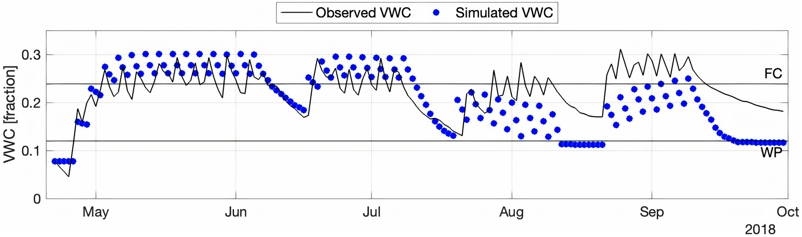
For example, it is possible actual ET was greater than the crop water requirement, causing the modeled VWC to show comparatively drier soil conditions than the observed. During the nonirrigated periods, evident when soil moisture decreases, VWC reached the wilting point (WP). The wilting point describes the point at which a given crop is unable to extract water due to soil suction pressure. At this point, the model prevents the water balance from subtracting ET for that layer (i.e., root water extraction) because the model does not explicitly account for possible reduction in SWS due to soil evaporation. The majority of deep infiltration losses occurred when VWC was above field capacity, where soil water mechanics are dominated by gravitational drainage.
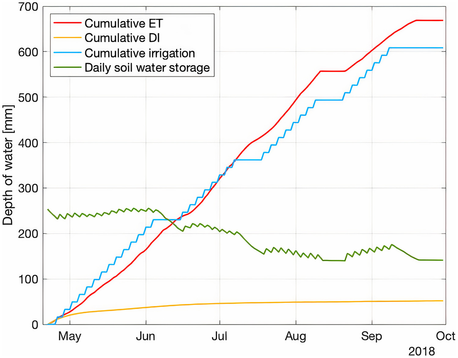
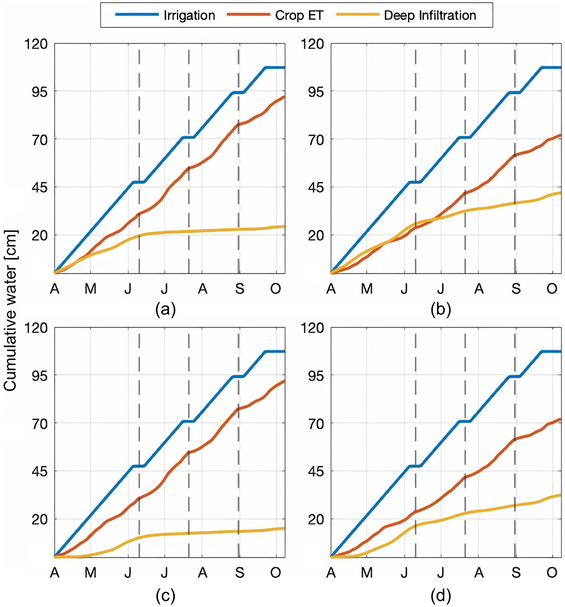
Overall, simulated DI from the 2018 calibration run (Fig. 1) was about 8% of total irrigation. A simulated water balance for the DI model is shown in Fig. 2, where depth of each major input and output can be compared over the length of the growing season. As the distance between cumulative root water extraction and irrigation decreases, applied irrigation more accurately replaces the crop water requirement. As a result, deep infiltration will be minimal. The change in soil water storage corresponds to flat periods on the cumulative irrigation plot when irrigation is shut off and alfalfa is cut. Overall, total soil water storage in the root zone decreased by about 10 cm by the end of the season, of which part can be attributed to the ET in excess of applied irrigation.
Magic Valley Soil Parameters
In order to represent Magic Valley soils where alfalfa is grown, soil spatial data were retrieved from Soil Web, an online mapping tool that utilizes the USDA-NRCS Web Soil Survey database (Soil Survey Staff, n.d.). Areas irrigating alfalfa in 2019 were identified using the USDA National Agriculture Statistics Service CropScape interface (USDA-NASS 2024). Soil spatial layers were then masked using irrigated alfalfa fields, and categorized into three groups (i.e., well-drained, poorly drained, and excessively drained) based on their drainage descriptions in web soil survey. An area-weighted average was used to determine soil texture values (i.e., percentage of sand, clay, and organic matter) for each soil group. Texture compositions were then used within regression equations to determine moisture content at FC, MAD, and WP (Saxton and Rawls 2006).
Soil drainage parameters and [Eq. (2)] were determined for each soil group. The drainage constant was determined by estimating saturated hydraulic conductivity () at the beginning of the decay curve, where SWS is represented as a function of time (Ogata and Richards 1957) as follows:where = time (days); = water storage (mm); = intermediate water content between FC and SAT; and = negative drainage constant. Table 3 gives the range of values determined for each soil group, and the approximate values and class descriptions from the National Soil Survey Handbook (USDA 2021). For all soil groups, the constant was set as . Because and constants are functions of soil texture, each layer of the model can be assigned specific values. For Magic Valley scenarios, soil texture was assumed homogenous through the root zone. The root zone was divided into three layers for alfalfa; the top layer depth from the surface to 20 cm, and two underlying layers each 50 cm thick (20–70 and 70–120 cm, respectively), resulting in a total effective root zone depth of 120 cm.
(12)
The percent of root extraction occurring at each layer depth was parameterized using a linear scaling factor [Eq. (10)]. Lastly, antecedent or initial SWS was set at field capacity for half of tested scenarios, and at management allowable depletion for the other remaining scenarios. This was to account for variability in precipitation during winter months in southern Idaho, which can play a role in initial SWS at the start of the growing season.
| Soil group | Description | SAT (% by volume) | FC (% by volume) | WP (% by volume) | constant (% by volume) | constant | ()a | class (1993)a |
|---|---|---|---|---|---|---|---|---|
| SC1 | Well-drained, silt loam | 38 | 26 | 10 | 30 | (, ) | (2.30, 12.20) | Moderately high to high |
| SC2 | Poorly drained, clay loam | 38 | 18 | 7 | 25 | (,) | (0.20, 0.90) | Very low to moderately low |
| SC3 | Excessively-drained, sandy loam | 35 | 15 | 10 | 21 | (, ) | (23.20, 50.40) | High to very high |
Note: Field capacity (FC), saturation (SAT), and wilting point (WP) in volumetric water content were determined for each soil group.
a
National Soil Survey Handbook, Figure 618-A25 (USDA 2021).
Reference ET, Reference ET Fraction, and Irrigation
Two growing seasons (2015 and 2019) were used to determine reference ET () and reference ET fraction time series to account for climatic variables affecting crop growth and transpiration. Daily alfalfa data from April 1 to October 9 were downloaded from the AgriMet station at Kimberly, Idaho, with station identifier TWFI (US Bureau of Reclamation 2021). AgriMet is a weather station network operated by the Bureau of Reclamation which provides an estimation of crop water use following the ASCE equation (Allen et al. 2005). Two reference ET fraction (ETrF) time series were created based on three alfalfa harvests, and actual ET () for years 2015 and 2019. In this study, ETrF is applied in a similar way as the crop coefficient (Allen et al. 1998), where a fraction is used to adjust . In choosing 2015 and 2019, 2 years that showed high and low atmospheric water demand, respectively, ETrF was used as a simplified term to capture a wide range of crop responses and evaporative conditions.
for irrigated alfalfa was determined using a gridded map product provide by Idaho Department of Water Resources (IDWR 2021). These maps of were generated using the surface energy model mapping evapotranspiration at high resolution and internalized calibration (METRIC) (Allen et al. 2011). Thermal band and visual scenes from Landsat were calibrated within METRIC to account for the range of observed pixel temperatures. A time series of ET values for each pixel was interpolated between scenes to create a map of total seasonal . Daily estimates of METRIC and AgriMet were summed over the length of the growing season, and the ratio of total to was determined for 2015 and 2019. This ratio is the seasonal ETrF average and was used to adjust the daily ETrF time series for each year until the area above and below the ratio line was equal (Fig. 3).
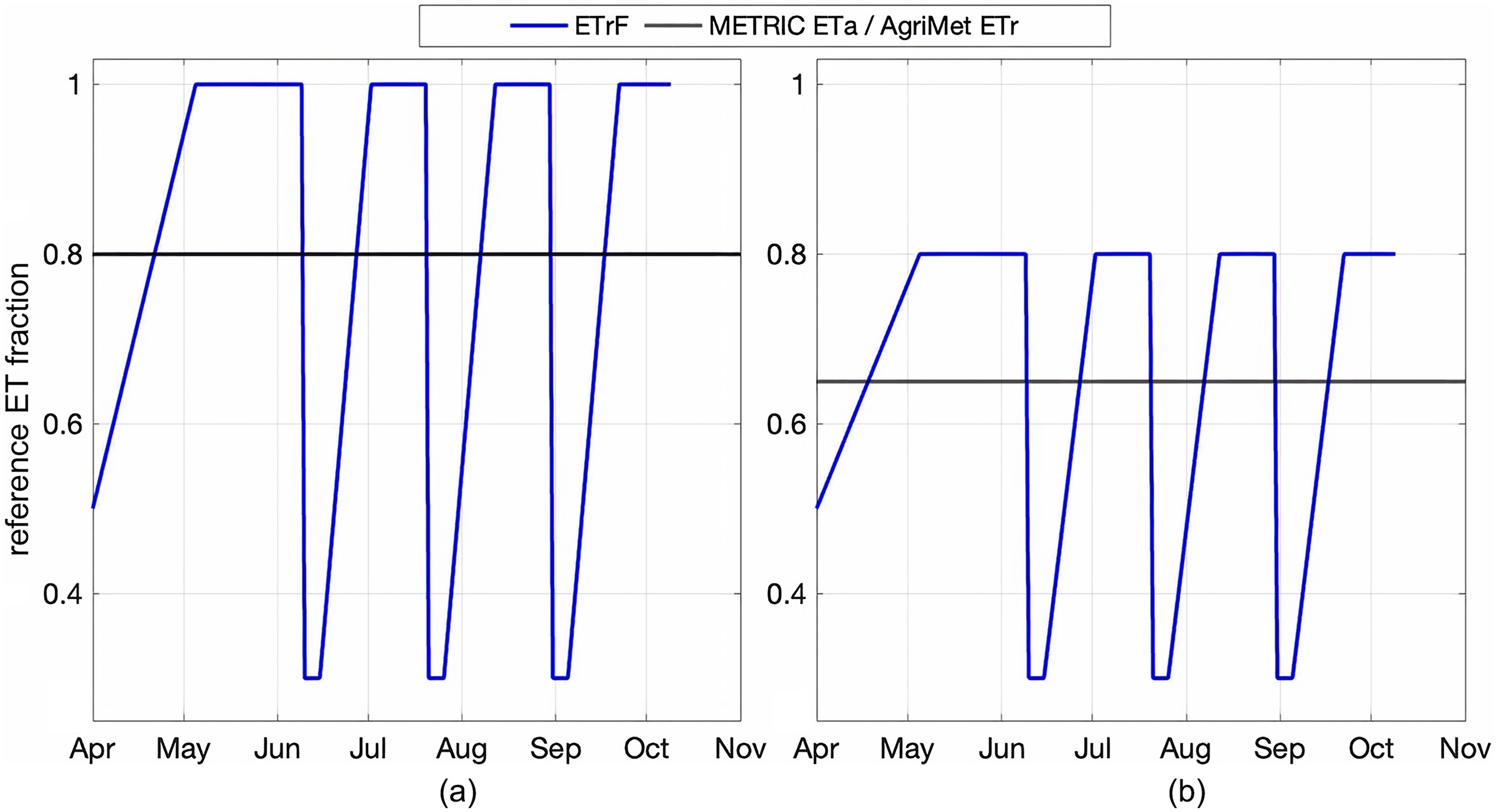
Fig. 3(a) shows the dry growing season where the range of ETrF values is greatest (hereafter referred as ET1). This represents years where atmospheric demand for water is high, and ETrF = 1 indicating full evaporative potential from the crop. Fig. 3(b) shows where maximum ETrF is suppressed, indicating a wet growing season (hereafter ET2). ET2 makes a simplifying assumption that crop water requirements are lower in seasons with increased humidity or cloud cover.
An irrigation schedule was created based on typical flow rates for center-pivot systems operated in Magic Valley (Hines and Neibling 2013). Although irrigators are constrained by the upper limits of applications depths based on system flow rates, pivot speed can be manually adjusted, which alters application depth and the time required for the pivot to make a full rotation. Generally, southern Idaho experiences arid, hot growing seasons requiring constant application of water. As such, a 1-day irrigation schedule was developed to apply 0.32 in. (0.80 cm) to the entire field within 24 h. To test pivot system application efficiency, a range of 72% to 90% was tested for each scenario; AE reduces the irrigation application depth, assuming 0.32 in. (0.80 cm) is delivered to the soil surface when AE is 100%. In the model, AE reduces the effective irrigation, or irrigation that increases soil water storage.
Consumptive-Use and Water Use Efficiency
Twelve scenarios based on Magic Valley soil texture, initial soil water storage, irrigation system efficiency, and atmospheric water demand were evaluated using the Deep Infiltration model in MATLAB software (Release 2021a) (Table 4). For each scenario, the range of application efficiency values (10 total) and drainage rates (10 total) were run mechanistically, resulting in 1,200 model runs. MATLAB was used to generate figures and calculate model results in terms of irrigation efficiency. For this study, consumptive use efficiency (CUE) is defined as follows:where Irr = depth daily irrigation (mm); and AE = application efficiency (fraction). Irrigation multiplied by the application efficiency accounts for effective irrigation added to the soil. DI is summed over the length of the season, as well as the total scheduled irrigation, which is multiplied by a constant seasonal AE value for a given model run. The ratio is subtracted from one to represent the amount of water efficiency stored in the root zone and used directly in meeting the consumptive use requirement. CUE is multiplied by the application efficiency to represent total water use efficiency (WUE), a metric describing all sources of water loss after irrigation is conveyed to the farm
(13)
(14)
| Scenario | Description | ET/ETrF time series | Initial SWS |
|---|---|---|---|
| Dry winter, arid summer | Little preseason soil water recharge and hot summer with high evaporative demand | ET1 | SWS at MAD |
| Wet winter, arid summer | Ample preseason soil water storage and hot summer with high evaporative demand | ET1 | SWS at FC |
| Dry winter, humid summer | Little preseason soil water recharge and mild summer with low evaporative demand | ET2 | SWS at MAD |
| Wet winter, humid summer | Ample preseason soil water storage and mild summer with low evaporative demand | ET2 | SWS at FC |
Note: Two reference ET fraction (ETrF) time series were developed, ET1 describing high atmospheric water demand and low water demand, and ET2. Initial soil water storage (SWS) is set near management allowable depletion (MAD) for half of scenarios, and near field capacity (FC) for remaining scenarios. Each scenario is mechanistically tested for three soil groups (Table 3), equaling 12 total scenarios.
Assuming CUE is water consumed through ET versus water delivered to the soil, WUE is then defined as the ratio of water used by the crop to water delivered to the farm. This metric accounts for inefficiencies such as deep infiltration and assumes aboveground losses are due to wind loss, soil evaporation, and runoff. These aboveground losses are not explicitly accounted for in the model but are the assumed losses before effective irrigation is delivered to the soil (i.e., AE).
Results and Discussion
Deep Infiltration
The amount of infiltration draining vertically from the bottom of the soil profile was summed over the length of the growing season. Deep infiltration, as a percentage, is the total seasonal infiltration divided by total effective irrigation. For each model run, the same amount of scheduled irrigation (i.e., irrigation before AE is considered) was used. It was found that for all scenarios, DI increased with higher application efficiency (Fig. 4). Results present DI tested under a range of drainage rates or hydraulic conductivities ( parameter in Table 3). DI increased across application efficiency for all soil groups and most drainage rates; the exception being SC3 tested at a high drainage rate. DI losses were greatest for SC2 and SC3 soils under the wet winter, humid summer scenario [Fig. 4(b)].
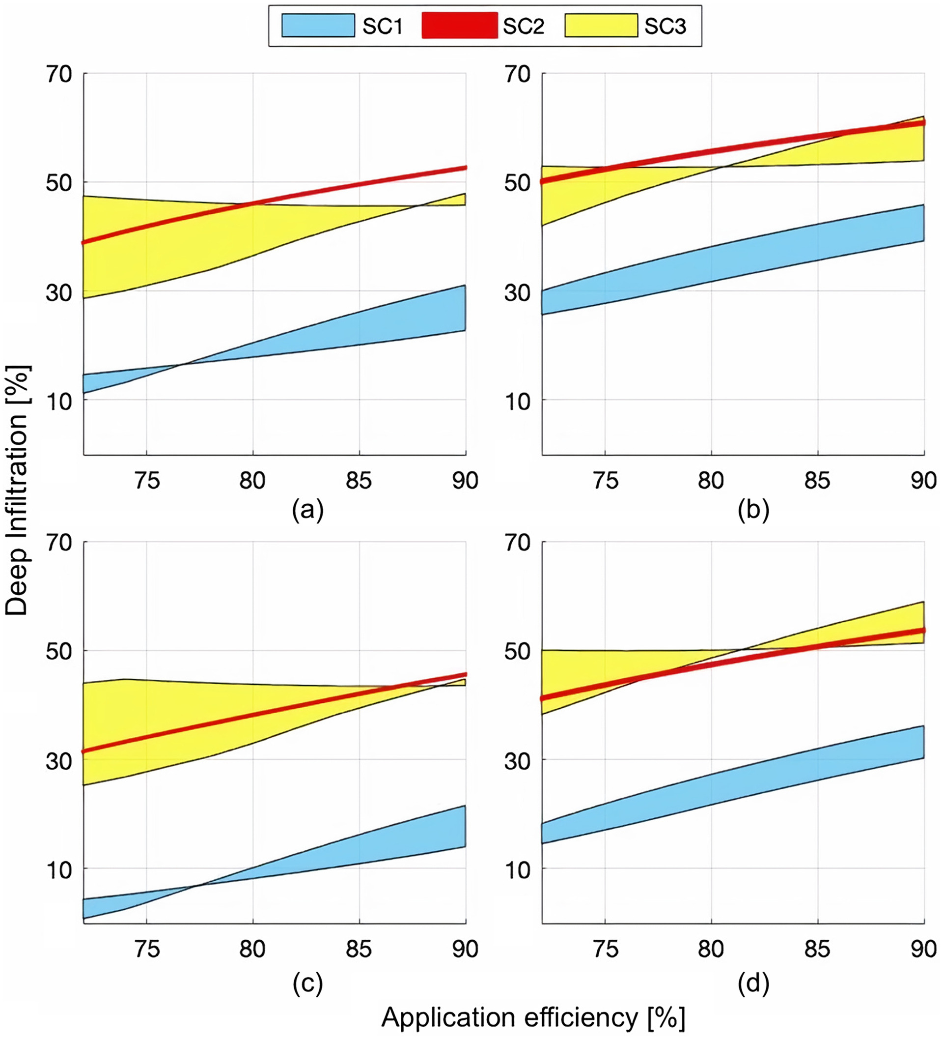
DI is conditional on several factors including SWS, water-holding capacity, ET requirement, and the rate of drainage. Deep infiltration was highest for SC2 and SC3; the water-holding capacity for these soils are between 5% and 11%, which limits the amount of available soil water under the wet winter, humid summer scenario. The wet winter, humid summer scenario not only recharges the soil profile before the irrigation season, but also decreases the amount of root water extraction due to a lower ET requirement. DI is thus magnified for SC2 and SC3 tested under slower drainage rates for this scenario. In contrast, the dry winter, arid summer scenario reduced total seasonal DI because effective irrigation was optimal in refilling the soil profile and meeting a higher ET requirement [Fig. 4(c)].
Drainage rates showed a notable effect on DI, which was evident as DI occurred at a faster rate for high hydraulic conductivity than for low hydraulic conductivity. The drainage rates used in the model are comparable to reported values of saturated hydraulic conductivity presented in Table 3. The results agree with expectation that infiltration would occur most often with high hydraulic conductivity. Rapid drainage occurs when SWS is above field capacity and approaching saturated soil conditions. As application efficiency increases, SWS increases because more effective irrigation is added to the root zone (Fig. 4). Soils with larger soil water reservoirs will typically experience less DI because they are able to retain water for longer periods of time. Soils with smaller soil water-holding capacities showed increased persistence of DI because soil water storage is likely rise above field capacity more often.
SC3 showed a different response to DI for tested scenarios; at high drainage rates, DI decreased or remained constant with increased application efficiency. A decrease in DI only occurred for SC3 under the dry winter, arid summer scenario [Fig. 4(c)]. For other scenarios, SC3 at high drainage rates showed constant DI regardless of application efficiency. SC2 or poorly drained soils showed less variation in DI losses with tested drainage rates. These results suggest excessively drained sandy soils and poorly drained clay loams present challenges in managing for DI losses due to the combined effect of drainage rates and water-holding capacity.
The influence of initial SWS on deep infiltration was notable in the model results, especially its effect on the incidence and recurrence of DI during the growing season. Fig. 5 shows cumulative DI (depth) for well-drained soils tested at an application efficiency of 90%; according to the model design, the pivot system will deliver 90% of applied irrigation to the root zone. It was found that regardless of application efficiency, 65% to 70% of total DI losses occurred before the first cutting under the wet winter, humid summer scenario [Fig. 5(b)]. Initial SWS was set at field capacity for this scenario, causing early season irrigation to exceed the ET requirement and soil water deficit during this period. As the gap between cumulative irrigation and modeled crop ET (i.e., root water extraction) increased, cumulative seasonal DI losses also increased.
When the ET requirement was increased but initial SWS remained at field capacity [Fig. 5(a)], most DI occurred before the first cutting but remained low during the hot summer months. This suggests that for wet winter conditions, irrigation management can reduce DI losses by accounting for early season soil water storage. This accounting is done using soil moisture probes and field-scale water balance methods to determine the soil water deficit.
Consumptive-Use Efficiency
One goal in improving irrigation systems is to increase water use efficiency and reduce consumptive use while ensuring the crop is adequately watered. To evaluate these criteria under different climatic and environmental scenarios, CUE was calculated across the range of application efficiencies [Eq. (13)]. CUE serves as a metric to evaluate what portion of the applied water is used for beneficial purposes, which is assumed to equal both root water extraction and crop ET. This calculation assumed other losses (such as surface runoff, wind loss, and soil evaporation) are represented by the range of application efficiencies. Because percent deep infiltration (Fig. 4) is directly related to CUE, Fig. 6 mirrors the previous patterns observed across the range of tested application efficiency.
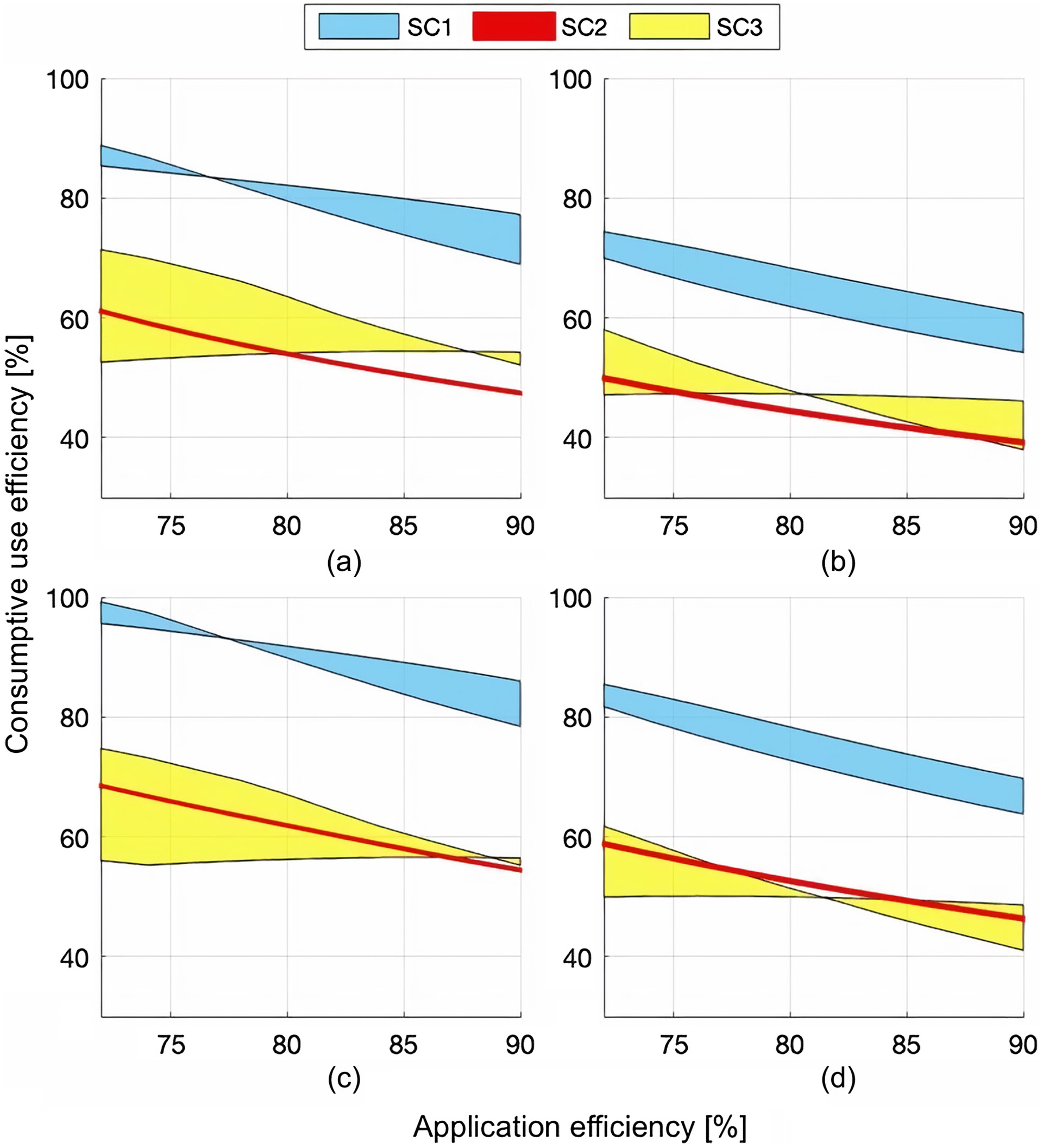
It was found CUE decreased with increased application efficiency for all scenarios and soil groups (Fig. 6). SC3 demonstrated the only exception to this pattern, where CUE increased slightly or remains constant with higher drainage rates. CUE was optimal for silt loam (SC1) tested under the dry winter, arid summer scenario with values between 80% and 100% [Fig. 6(c)]. Silt loams were the most prevalent soils used to irrigate alfalfa in the Magic Valley, suggesting these soils are generally the most productive. Results for SC1 support this idea because high CUE indicates the model used irrigation primarily for meeting the ET requirement. SC1 model runs were also parameterized with a larger water-holding capacity, which is ideal for supporting crops during arid periods of the summer. It is also likely the range of drainage rates tested for SC1 aided in the timely refill and distribution of water through the soil profile. In contrast, SC3 or excessively drained soils showed a high negative rate of CUE to application efficiency tested under high hydraulic conductivity. Under these soil conditions, the holding capacity and the rate of drainage limit available soil water.
At the lower end of application efficiency, CUE was highest among model runs. Because AE decreases the amount of effective irrigation added to the root zone, soil water storage and potential deep infiltration also decreased. In this simplified accounting, effective irrigation at low AE more closely matched the ET requirement and the soil water deficit under a given scenario. The effective irrigation at 72% AE was closely matched to crop and soil water requirements for the dry winter, arid summer scenario [Fig. 6(c)]. Because all model runs showed decreased CUE with increased application efficiency, this indicates the scheduled irrigation was set higher than the ET and soil water requirement for tested scenarios.
One possible extension from this study would be to evaluate DI for different irrigation schedules or decreased application depths. These model outcomes could support the idea that consumptive use efficiency is optimal when more efficient irrigation systems are coupled with precision agriculture techniques such as limiting application to the observed ET, and by monitoring actual soil water content. Precision methods like irrigation scheduling and field-scale water balances are not always convenient or affordable. They require both time and skilled labor to implement effectively while still ensuring that crops are adequately watered.
All the same, the results suggest adoption of modified irrigation systems alone do not guarantee CUE increases if not also coupled with irrigation scheduling that matches the ET requirement and the soil capacity. The benefit of modified systems is aboveground water losses are decreased. By adopting systems that apply water closer to the soil surface, more water is likely to be delivered to the soil profile, even if the fate of the water is not entirely clear.
Water Use Efficiency
WUE was evaluated by multiplying consumptive use efficiency by application efficiency [Eq. (14)], which describes the ratio of water consumed by ET to water delivered to farm. It was found for SC1 and SC2 soils, WUE increased with application efficiency for some scenarios and drainage rates (Fig. 7). SC1 showed the highest WUE among soil groups and scenarios when weather conditions were humid [Figs. 7(a and c)]. SC3 showed the widest range of variability, with increased WUE for all scenarios and certain drainage rates. SC2 or clay loam poorly drained soils showed constant WUE across application efficiencies, except a slight decrease under the dry winter, arid summer scenario [Fig. 7(a)].
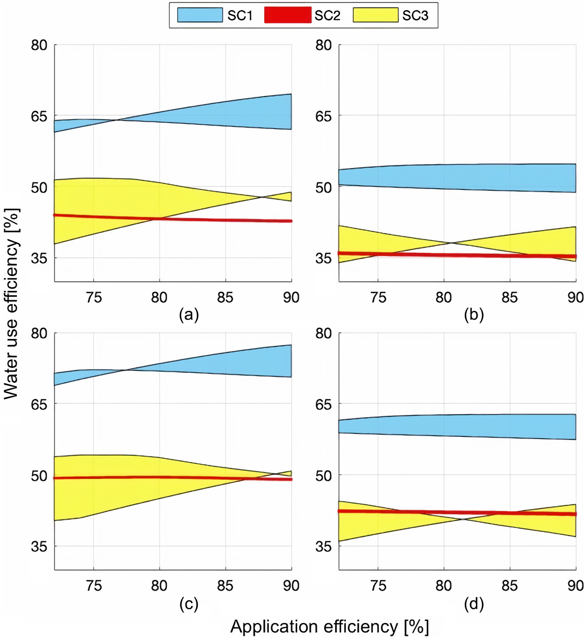
The model demonstrated that water use efficiency can be improved marginally under certain climatic scenarios and for certain soil groups. Well-drained soils (SC1) showed the highest WUE potential, increasing in efficiency by 10%–15% under arid conditions [Fig. 7(a)]. SC3 showed some potential for increased efficiency depending on hydraulic conductivity of the soil. Clay loams (SC2) showed no improvement or decreased WUE under tested environmental conditions.
Conclusion
The deep infiltration model was designed using a simple water balance method, soil drainage function, and root water extraction functions to estimate soil water loss below the root zone for irrigated crops. Scenarios were created to encompass a range of soil groups and climatic conditions under which alfalfa could be grown in the Magic Valley, Idaho. It was found that DI generally increased with higher AE. Consumptive use efficiency, the fraction of effective irrigation used to meet the crop water demand, decreased with increased AE. Soil textures and drainage rates had a discernible effect on total seasonal DI. SC1 or well-drained soils performed the best among soil groups and across test scenarios.
The results suggest that well-drained soils show the most potential for improved water use efficiency and irrigation management to reduce DI. Excessively drained and poorly drained soils tested within the model pose challenges in managing soils for decreased DI; this is due to low water-holding capacity and hydraulic conductivity rates that do not coincide with the timing of root water extraction. Modeled irrigation was generally higher than the ET requirement and soil water deficit for all scenarios. Future model implementation could test lower rates of irrigation application or varying speeds of center-pivot rotation to investigate the system efficiency of deficit irrigation or other schedule-based techniques.
This study suggests that modified systems with higher application efficiencies do not always improve water use efficiency; irrigation scheduling and water balance methods should also be used in order to meet crop ET in each specific location and condition. This model has practical applications by providing rapid and readily obtained estimates of deep infiltration. Understanding the magnitude of infiltration over broad geographic extent is essential to understanding impacts to water quality and quantity in soil water storage and groundwater recharge. The methods used in this model provide an order-of-magnitude quantification of near-surface boundary conditions and highlight the need for more consideration of infiltration losses in comprehensive modeling of regional water budgets.
Data Availability Statement
Some or all data, models, or code that support the findings of this study are available from the corresponding author upon reasonable request (MATLAB model code available).
Acknowledgments
Publicly available data obtained from Idaho Department of Water Resources (ET map data), and the Bureau of Reclamation AgriMet program (weather data) were essential for research presented in this project and serve as invaluable public sources of information for water resources research and management. The authors would also like to thank Drs. Richard Jasoni and Justin Huntington for providing field data used in model calibration. Research presented in this paper was supported by the University of Idaho, Department of Soil and Water Systems and partially by a NASA-Jet Propulsion Lab agreement with the University of Idaho #1667004 entitled “Accuracy Assessment of Satellite-based ET mapping for improved water and nutrient management in the Magic Valley”. This publication was partially developed under Agreement No. 2020-69012-3871, funded by the US Department of Agriculture (USDA), National Institute of Food and Agriculture and through funding from the NASA-Jet Propulsion Lab Western Water Applications Office.
Disclaimer
The authors declare no competing interests in the research or publication of this article. The funders of this research have no role in designation of topic, writing, or publication. No AI tools or LLMs were used in the preparation of this manuscript.
References
Allen, R. G., A. Irmak, R. Trezza, J. M. H. Hendrick, W. Bastiaanssen, and J. Kjaersgaard. 2011. “Satellite-based ET estimation in agriculture using SEBAL and METRIC.” Hydrol. Processes 25 (26): 4011–4027. https://doi.org/10.1002/hyp.8408.
Allen, R. G., L. S. Pereira, D. Raes, and M. Smith. 1998. “FAO irrigation and drainage paper No. 56.” Rome Food Agric. Organ. U. Nations 56 (97): 26–40.
Allen, R. G., I. A. Walter, R. L. Elliot, T. A. Howell, D. Itenfisu, M. E. Jensen, and R. L. Snyder. 2005. The ASCE standardized reference evapotranspiration equation. Reston, VA: ASCE.
Al-Oqaili, F., S. P. Good, R. T. Peters, C. Finkenbiner, and A. Sarwar. 2020. “Using stable water isotopes to assess the influence of irrigation structural configurations on evaporation losses in semiarid agricultural systems.” Agric. For. Meteorol. 291 (Jun): 108083. https://doi.org/10.1016/j.agrformet.2020.108083.
Arnold, J. G., et al. 2012. “SWAT: Model use, calibration, and validation.” Trans. ASABE 55 (4): 1491–1508. https://doi.org/10.13031/2013.42256.
Arnold, L. R. 2011. Estimates of deep-percolation return flow beneath a flood- and a sprinkler-irrigated site in Weld County, Colorado, 2008–2009. Reston, VA: USGS.
Calera, A., I. Campos, A. Osann, G. D’Urso, and M. Menenti. 2017. “Remote sensing for crop water management: From ET modelling to services for the end users.” Sensors 17 (5): 1104. https://doi.org/10.3390/s17051104.
Campbell Scientific. 2008. “Energy balance and water flow determination with the eddy covariance method.” Accessed May 13, 2024. https://s.campbellsci.com/documents/fr/technical-papers/edire.pdf.
Campbell Scientific. 2020. “CS616 water content reflectometer: Instruction manual.” Accessed November 29, 2023. https://s.campbellsci.com/documents/au/manuals/cs616.pdf.
Contor, B. A., and R. G. Taylor. 2013. “Why improving irrigation efficiency increases total volume of consumptive use.” Irrig. Drain. 62 (Mar): 273–280. https://doi.org/10.1002/ird.1717.
Cosgrove, D. M., B. A. Contor, and G. S. Johnson. 2006. Enhanced snake plain aquifer model final report. Moscow, ID: Idaho Water Resources Research Institute, Univ. of Idaho.
Ferreira, A., J. Rolim, P. Paredes, and M. Cameira. 2022. “Assessing spatio-temporal dynamics of deep percolation using crop evapotranspiration derived from earth observations through Google earth engine.” Water 14 (15): 2324. https://doi.org/10.3390/w14152324.
Gee, G. W., and D. Hillel. 1988. “Groundwater recharge in arid regions: Review and critique of estimation methods.” Hydrol. Processes 2 (Jun): 255–266. https://doi.org/10.1002/hyp.3360020306.
Gómez, D. G., C. G. Ochoa, D. Godwin, A. A. Tomasek, and R. Zamora. 2022. “Soil moisture and water transport through the vadose zone and into the shallow aquifer: Field observations in irrigated and non-irrigated pasture fields.” Land 11 (11): 2029. https://doi.org/10.3390/land11112029.
Grafton, R. Q., J. Williams, C. J. Perry, F. Molle, C. Ringler, P. Steduto, B. Udall, S. A. Wheeler, Y. Wang, D. Garrick, and R. G. Allen. 2018. “The paradox of irrigation efficiency.” Science 361 (Jun): 748–750. https://doi.org/10.1126/science.aat9314.
Hines, S., and H. Neibling. 2013. “Center pivot irrigation for corn: Water management and system design considerations in Southern Idaho.” Accessed June 1, 2021. https://www.lib.uidaho.edu/digital/uiext/items/uiext31492.html.
Hunink, J., M. Vila, and A. Baille. 2011. “REDSIM: Approach to soil water modelling.” In Tools and data considerations to provide relevant soil water information for deficit irrigation. Wageningen, Netherlands: FutureWater.
IDWR (Idaho Department of Water Resources). 2021. “Evapotranspiration (ET): 2019.” Idaho Department of Water Resources map and GIS data hub. Accessed March 1, 2021. https://data-idwr.hub.arcgis.com/documents/a0daa6011b4f4ae0a0d6ad4a11df9bed/about.
IDWR (Idaho Department of Water Resources). 2024. “IWRB financial programs.” Accessed January 3, 2024. https://idwr.idaho.gov/iwrb/programs/financial/.
Irmak, S., L. O. Odhiambo, W. L. Kranz, and D. E. Eisenhauer. 2011. Irrigation efficiency and uniformity, and crop water use efficiency. Lincoln, NE: Univ. of Nebraska.
Johnson, G. S., W. H. Sullivan, D. M. Cosgrove, and R. D. Schmidt. 1999. “Recharge of the Snake River Plain Aquifer: Transitioning from incidental to managed.” JAWRA J. Am. Water Resour. Assoc. 35 (Jun): 123–131. https://doi.org/10.1111/j.1752-1688.1999.tb05457.x.
Kliskey, A., J. Abatzoglou, L. Alessa, C. Kolden, D. Hoekema, B. Moore, S. Gilmore, and G. Austin. 2019. “Planning for Idaho’s waterscapes: A review of historical drivers and outlook for the next 50 years.” Environ. Sci. Policy 94 (May): 191–201. https://doi.org/10.1016/j.envsci.2019.01.009.
Konikow, L. F. 2013. Groundwater depletion in the United States (1900–2008). Reston, VA: USGS.
Lian, J., Y. Li, Y. Li, X. Zhao, T. Zhang, X. Wang, X. Wang, L. Wang, and R. Zhang. 2022. “Effect of center-pivot irrigation intensity on groundwater level dynamics in the agro-pastoral ecotone of northern China.” Front. Environ. Sci. 10 (Jun): 892577. https://doi.org/10.3389/fenvs.2022.892577.
Liu, Y., L. S. Pereira, and R. M. Fernando. 2006. “Fluxes through the bottom boundary of the root zone in silty soils: Parametric approaches to estimate groundwater contribution and percolation.” Agric. Water Manage. 84 (Jun): 27–40. https://doi.org/10.1016/j.agwat.2006.01.018.
Miller, K., P. Goulden, K. Fritz, M. Kiparsky, J. Tracy, and A. Milman. 2021. “Groundwater recharge to address integrated groundwater and surface waters: The ESPA recharge program, Eastern Snake Plain, Idaho.” Case Stud. Environ. 5 (1): 1223981. https://doi.org/10.1525/cse.2020.1223981.
Molaei, B., R. T. Peters, A. Z. Mohamed, and A. Sarwar. 2021. “Large scale evaluation of a LEPA/LESA system compared with MESA on spearmint and peppermint.” Ind. Crops Prod. 159 (Jan): 113048. https://doi.org/10.1016/j.indcrop.2020.113048.
Niswonger, R. G., K. K. Allander, and A. E. Jeton. 2014. “Collaborative modelling and integrated decision support system analysis of a developed terminal lake basin.” J. Hydrol. 517 (Jan): 521–537. https://doi.org/10.1016/j.jhydrol.2014.05.043.
Ogata, G., and L. A. Richards. 1957. “Water content changes following irrigation of bare-field soil that is protected from evaporation.” Soil Sci. Soc. Am. J. 21 (Mar): 355–356. https://doi.org/10.2136/sssaj1957.03615995002100040001x.
Olson, R., R. Budge, and T. J. Budge. 2016. “Summary of ESPA settlement agreement.” Accessed May 17, 2021. https://www.racinelaw.net/blog/summary-espa-settlement-agreement/.
Oregon Water Resources Department. 2020. “Water use reportingfrom.” Accessed June 1, 2020. https://apps.wrd.state.or.us/apps/wr/wateruse_queryhttps://apps.wrd.state.or.us/apps/wr/wateruse_query//.
Perry, C. 2007. “Efficient irrigation; inefficient communication; flawed recommendations.” Irrig. Drain. 56 (Mar): 367–378. https://doi.org/10.1002/ird.323.
Perry, C. J., P. Steduto, R. G. Allen, and C. Burt. 2009. “Increasing productivity in irrigated agriculture: Agronomic constraints and hydrological realities.” Agric. Water Manage. 96 (Mar): 1517–1524. https://doi.org/10.1016/j.agwat.2009.05.005.
Peters, R. T., G. Hoogenboom, and S. Hill. 2019. “Simplified irrigation scheduling on a smart phone or web browser.” In Proc., Irrigation Show. Fairfax, VA: Irrigation Association.
Peters, R. T., H. Neibling, and R. Stroh. 2016. Low energy precision application (LEPA) and low elevation spray application (LESA) trials in the Pacific Northwest. In Proc., 46th California Alfalfa and Forage Symp., 51–72. Davis, CA: Univ. of California.
Rajan, N., S. Maas, R. Kellison, M. Dollar, S. Cui, S. Sharma, and A. Attia. 2015. “Emitter uniformity and application efficiency for centre–pivot irrigation systems.” Irrig. Drain. 64 (Mar): 353–361. https://doi.org/10.1002/ird.1878.
Saxton, K. E., and W. J. Rawls. 2006. “Soil water characteristic estimates by texture and organic matter for hydrologic solutions.” Soil Sci. Soc. Am. J. 70 (Mar): 1569–1578. https://doi.org/10.2136/sssaj2005.0117.
Šimůnek, J. 2015. “Estimating groundwater recharge using HYDRUS-1D.” Eng. Geol. Hydrogeol. 29 (Mar): 25–36.
Soil Survey Staff. n.d. “U.S. general soil map (STATSGO2).” Accessed July 17, 2021. https://agdatacommons.nal.usda.gov/articles/model/United_States_General_Soil_Map_STATSGO2_/24660345.
Steduto, P., T. C. Hsiao, D. Raes, and E. Fereres. 2009. “AquaCrop—The FAO crop model to simulate yield response to water: I. Concepts and underlying principles.” Agron. J. 101 (3): 426–437. https://doi.org/10.2134/agronj2008.0139s.
Stewart-Maddox, N., P. Thomas, W. Parham, and W. Hipke. 2018. “Restoring a world class aquifer: A brief history behind managed recharge & conjunctive management.” Accessed August 1, 2021. https://www.arlis.org/docs/vol2/TheWaterReport/2018/TWR173_July_2018.pdf.
Stockle, C. O., S. A. Martin, and G. S. Campbell. 1994. “CropSyst, a cropping systems simulation model: Water/nitrogen budgets and crop yield.” Agric. Syst. 46 (Mar): 335–359. https://doi.org/10.1016/0308-521X(94)90006-2.
US Bureau of Reclamation. 2021. “AgriMet: The Pacific Northwest cooperative agricultural weather network.” Accessed March 1, 2021. https://www.usbr.gov/pn/agrimet/.
USDA. 2021. National soil survey handbook. Washington, DC: USDA.
USDA-NASS (National Agricultural Statistics Service). 2024. “Cropland data layer: USDA NASS marketing and Information Services Office, Washington, D.C.” Accessed June 1, 2022. https://croplandcros.scinet.usda.gov.
Vano, J. A., M. J. Scott, N. Voisin, C. O. Stöckle, A. F. Hamlet, K. E. B. Mickelson, M. M. Elsner, and D. P. Lettenmaier. 2010. “Climate change impacts on water management and irrigated agriculture in the Yakima River Basin, Washington, USA.” Clim. Change 102 (Mar): 287–317. https://doi.org/10.1007/s10584-010-9856-z.
Veihmeyer, F. J., and A. H. Hendrickson. 1931. “The moisture equivalent as a measure of the field capacity of soils.” Soil Sci. 32 (3): 181–194. https://doi.org/10.1097/00010694-193109000-00003.
Volk, J. M., et al. 2023. “Development of a benchmark eddy flux evapotranspiration dataset for evaluation of satellite-driven evapotranspiration models over the CONUS.” Agric. For. Meteorol. 331 (Mar): 109307. https://doi.org/10.1016/j.agrformet.2023.109307.
Ward, F. A., and M. Pulido-Velazquez. 2008. “Water conservation in irrigation can increase water use.” Proc. Natl. Acad. Sci. 105 (7): 18215. https://doi.org/10.1073/pnas.0805554105.
Information & Authors
Information
Published In

Journal of Irrigation and Drainage Engineering
Volume 150 • Issue 5 • October 2024
Copyright
This work is made available under the terms of the Creative Commons Attribution 4.0 International license, https://creativecommons.org/licenses/by/4.0/.
History
Received: Nov 16, 2023
Accepted: Apr 22, 2024
Published online: Jul 26, 2024
Published in print: Oct 1, 2024
Discussion open until: Dec 26, 2024
ASCE Technical Topics:
- Ecosystems
- Environmental engineering
- Geomechanics
- Geotechnical engineering
- Hydrologic engineering
- Hydrology
- Infiltration
- Irrigation
- Irrigation engineering
- Soil mechanics
- Soil properties
- Soil water
- Vegetation
- Water and water resources
- Water conservation
- Water management
- Water policy
- Water shortage
- Water supply
- Water use
Authors
Metrics & Citations
Metrics
Citations
Download citation
If you have the appropriate software installed, you can download article citation data to the citation manager of your choice. Simply select your manager software from the list below and click Download.