Response of Bedload and Bedforms to Near-Bed Flow Structures

Zhao, Chenwei; Fang, Hongwei; Ouro, Pablo; Stoesser, Thorsten; Dey, Subhasish

doi:10.1061/JHEND8.HYENG-13618

Open access

Technical Papers

Nov 10, 2023

Response of Bedload and Bedforms to Near-Bed Flow Structures

Authors: Chenwei Zhao [email protected], Hongwei Fang, M.ASCE https://orcid.org/0000-0002-5621-6279 [email protected], Pablo Ouro [email protected], Thorsten Stoesser, A.M.ASCE https://orcid.org/0000-0001-8874-9793 [email protected], and Subhasish Dey, M.ASCE [email protected]Author Affiliations

Publication: Journal of Hydraulic Engineering

Volume 150, Issue 1

https://doi.org/10.1061/JHEND8.HYENG-13618

PDF

Abstract

In this study, the large eddy simulation (LES) under the Eulerian method is used to solve the Navier-Stokes equations for turbulent flow simulation. The Lagrangian point-particle model is applied to track particle trajectories and to calculate the forces exerted by the flow on the particles, and the particle–wall and particle–particle collisions are also accounted for. Nine simulations cases were carried out along the line of previous experiments that considered different bedform regimes, namely, ripples and dunes. The resulting bedload intensity parameter and the simulated bedforms for all the cases agree with the results obtained from the existing classical formulas. The three-dimensionality of sediment transport randomly occurs due to the turbulent flow. Coherent structures are formed as the near-bed low-speed fluid streaks entrain into the mainstream over the stoss-side of the ripples, and the high-speed fluid streaks from the mainstream rush toward the bed over the leeside. As a result, kolk–boil and hairpin vortices develop nearby. Ejection and sweep prevail near the bed, where the particles transport. The phenomenon disappears as the flow intensity increases. The presence of bedload particles also modifies the propagation angle and range of velocity fluctuation, especially in the streamwise direction. To conclude, a logistic regression formula for bedload intensity parameters, accounting for the fluid rotation, deformation, and translation terms that signify the fluid vortical motions, is obtained. It reveals that as long as these three terms are accurately quantified, the bed shear stress and bedload transport rate can be effectively estimated.

Introduction

Bedload transport is one of the principal modes of sediment transport, along with suspended-load transport. It is especially significant in mountainous rivers having a gravel bed, where the dominant mode of sediment transport is the bedload. The bedload transport is governed by hydrodynamic action, contributing to the formation of riverbed morphology. Hence, it can, in turn, modify the flow characteristics. The bedload also influences pollutant and material transport (Huang et al. 2015; Fang et al. 2017) and the habitat of aquatic organisms (Pitlick and Van Steeter 1998; Bui et al. 2019). Therefore, it is of great scientific and engineering significance to study the mechanism of bedload transport precisely.

In the past, several researchers focused on the flow–sediment interaction, with the intention to provide an accurate bedload model for the prediction of bedload transport rate. Some of the previous bedload formulas are based on a saltation concept as the product of the saltating particle velocity, saltation height, and volumetric particle concentration, to obtain the bedload transport rate (van Rijn 1984). The saltating particle velocity can be derived from the near-bed flow velocity, making the bedload transport rate a function of the near-bed instantaneous flow velocity, which in fact remains spatially heterogeneous. Other types of empirical formulas are based on the excess bed shear stress concept, called the du Boys equation (Dey 2014). The excess bed shear stress is defined as the difference between the bed shear stress

τ_{0}

induced by the flow and the threshold bed shear stress

τ_{c}

for the initiation of sediment particle motion. One of the celebrated formulas of bedload transport rate is known as the Meyer-Peter and Müller (1948) formula. In addition, Diplas et al. (2008) studied the conditions for sediment incipient motion and found that it is decided by the impulse. Wilcock (1998) studied the initial sediment motion of nonuniform sediment.

With the development of experimental techniques and numerical simulations, researchers have been motivated to study the bedform development for the prediction of dune dimensions, which are important for forecasting riverbed dynamics. Tjerry and Fredsøe (2005) theoretically studied the geometry of dunes by using a

k - ε

turbulence closure scheme. The results revealed that, at a low bed shear stress, the streamline curvature plays a key role in determining the location of maximum sediment transport due to an overshoot in bed shear stress. On the other hand, at a high bed shear stress, the downstream decay of turbulence from the former dune plays a major role. Khosronejad and Sotiropoulos (2014) developed a coupled hydro-morphodynamic model for carrying out large-eddy simulation of a stratified, turbulent flow over a sediment bed, based on the curvilinear immersed boundary approach to simulate bedform initiation, growth, and evolution. More detailed flow–sediment interaction has been unveiled by Bui and Rutschmann (2010), Pu and Lim (2014), and Pu et al. (2014). Notably, the identification of turbulent bursting phenomena in a wall-bound flow (Kline et al. 1967) has created a new ground to explore the sediment transport problem. A large number of studies have shown that turbulent coherent structures play a crucial role in transporting sediment particles (Jackson 1976; Heathershaw and Thorne 1985; Kaftori et al. 1995; Cao 1997; Bagherimiyab and Lemmin 2012). Among the bursting events, ejection and sweep are recognized to be the main events contributing to sediment transport, because they deliver a positive contribution to the Reynolds shear stress. However, quite a few studies have revealed that the Reynolds shear stress is not the most pertinent factor to oversee the bedload transport, which is associated with instantaneous streamwise velocity (Clifford et al. 1991; Papanicolaou et al. 2001, 2002; Schmeeckle and Nelson 2003). Specifically, it has been recognized that the transport of sediment particles is mainly controlled by the ejection events formed in the near-bed flow zone in the form of an arrival of low-speed fluid streaks (Drake et al. 1988; Dey et al. 2011, 2012). Bradley and Venditti (2017) compiled a literature review to examine our current understanding of the controls on dune dimensions in rivers via a meta-analysis of dune scaling relations.

Despite a number of serious attempts, the role of the near-bed flow structures on the bedload transport and bedforms has yet to be ascertained. This study, therefore, reveals how the bedload transport and the bedforms are influenced by the near-bed flow structures. In addition, the bedload transport rate is effectively quantified in terms of the fluid rotation, deformation, and translation terms. The turbulent flow is simulated in an infinite rectangular open channel and a large number of sediment particles are assumed to be spherical, implying that the effect of nonsphericity is neglected.

Numerical Framework

In this study, the large eddy simulation (LES), an in-house Hydro3D code, was used to simulate the turbulent flow in an open channel, which has been verified by previous researchers to be applicable to solve many complex flow phenomena (Bai et al. 2013; Liu et al. 2017; Nikora et al. 2019; Zhao et al. 2020).

The continuity and the Navier-Stokes (NS) equations for incompressible fluid flow were used as the governing equations. A force term was added to the momentum equation (NS), representing the feedback force exerted by the particles on the fluid. These equations read

\frac{\partial u_{i}}{\partial x_{i}} = 0

(1)

\frac{\partial u_{i}}{\partial t} + u_{j} \frac{\partial u_{i}}{\partial x_{j}} = - \frac{1}{ρ} \frac{\partial p}{\partial x_{i}} + 2 υ \frac{\partial S_{i j}}{\partial x_{j}} - \frac{\partial τ_{i j}}{\partial x_{j}} + f_{p, i}

(2)

where

u_{i} [= (u, v, w) for i = (1, 2, 3)]

are the velocity components in the

i

-direction;

x_{i} [= (x, y, z) for i = (1, 2, 3)]

are the coordinates;

p

= instantaneous pressure;

ρ

= fluid mass density;

υ

= fluid kinematic viscosity; and

f_{p, i}

= total force per unit volume exerted by the particles on the fluid in the

i

-direction. The Cartesian coordinates,

x

,

y

, and

z

, are the streamwise (horizontal), spanwise, and vertical distances, respectively. In addition,

S_{i j}

is the strain-rate tensor, given by (

\partial u_{i} / \partial x_{j} + \partial u_{j} / \partial x_{i}) / 2

;

τ_{i j}

is the subgrid stress (SGS) tensor, given by

2 υ_{t} S_{i j}

; and

υ_{t}

is the SGS viscosity. The wall-adapted local eddy viscosity (WALE) model was used to compute the SGS viscosity

υ_{t}

(Nicoud and Ducros 1999). A fourth-order central difference scheme (CDS) was applied to approximate the convective and diffusive velocity terms, and the fractional step method, called the explicit three-step Runge-Kutta scheme, was used for the time advancement (Cevheri et al. 2016).

The Lagrangian point-particle model (Balachandar 2009; Liu et al. 2019) was applied to compute the trajectories of the sediment particles. The governing equations, which can simulate the translational and rotational motions of particles during saltation, are Newton’s second law and the Euler equations. The equation for translational motion obtained from Newton’s second law is

m_{p} \frac{d u_{p, i}}{d t} = F_{p, i}

(3)

where

m_{p} = (ρ_{s} + C_{m} ρ) π d_{p}^{3} / 6

represents the total mass of the particle, including an added mass with an added mass coefficient

C_{m} = 0.5

(van Rijn 1984);

ρ_{s}

= particle mass density;

d_{p}

= nominal particle diameter;

u_{p, i}

= particle velocity in the

i

-direction; and

F_{p, i}

= total force acting on the particle in the

i

-direction, including the particle submerged weight, hydrodynamic drag force, hydrodynamic lift force, bed friction force, and Basset force. The detailed method was reported in Zhao et al. (2022) in the section “Lagrangian Model of Particle Saltation.”

The equation for rotational motion obtained from the Euler equation is

I_{p} \frac{d ω_{p, i}}{d t} = N_{p, i}

(4)

where

ω_{p, i}

= particle angular velocity about the

i

-axis;

I_{p} = m_{p} d_{p}^{2} / 10

represents the moment of inertia of the particle;

t

= time; and

N_{p, i}

= torque about the

i

-axis.

Particle–wall and particle–particle collisions were also introduced in the model with a friction coefficient of 0.89. The detailed method was reported in Zhao (2021).

Numerical Setup and Boundary Conditions

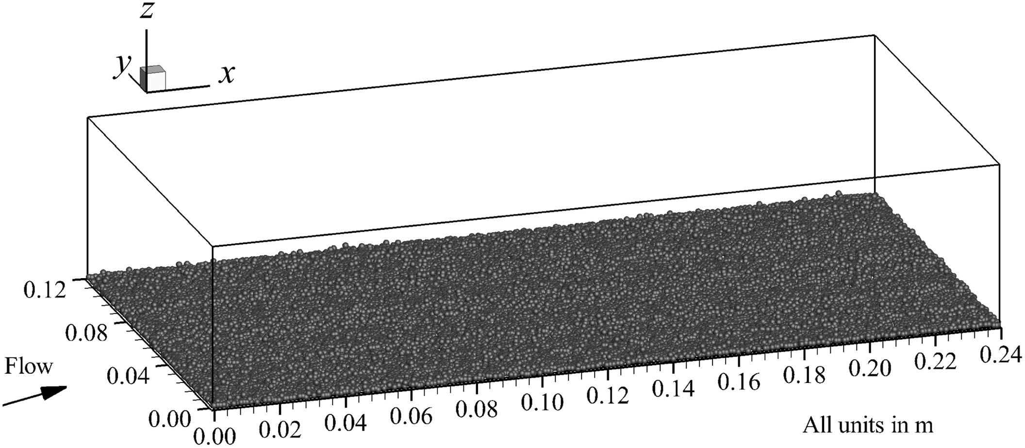
The simulations were carried out in the Sunway TaihuLight supercomputer at Tsinghua University, Beijing, China. Cases with a thin layer of bedload were simulated in a rectangular open channel with a size of

0.24 \times 0.12 m^{2}

(

length \times width

) using 72 processors, as shown in Fig. 1. A uniform grid with a size of

0.8 \times 0.8 \times 0.8 {mm}^{3}

was used. The flow conditions in experiment S12 of Niño and García (1998) were first used in Case T0, as the saltation model established by Zhao et al. (2020). Then, the other eight simulations for Cases T1–T8 were carried out in a series considering some experiments, which focused on the bed patterns as in Robert and Uhlman (2001) and Schindler and Robert (2005). All the related parameters of each case are outlined in Table 1. The flow depth

h

varied from 0.0352 to 0.264 m and mean flow velocity

u_{0}

from 0.318 to

0.96 m s^{- 1}

. The corresponding flow Reynolds numbers

R e

(

= u_{0} h / υ

, where

u_{0}

is the area-averaged flow velocity) were in the range of 11,201 to 253,440, and the flow Froude numbers

F r

[

= u_{0} / {(g h)}^{0.5}

, where

g

is the gravitational acceleration] were between 0.36 and 0.6. Approximately 30,000 mobile particles, having

d_{p} = 0.5 mm

(uniform) and

ρ_{s} = 2,650 kg m^{- 3}

, were laid as a thin layer on the bed with a zero-velocity at the beginning. Hence, the Shields parameters

Θ

, given by

u_{*}^{2} / g R^{'} d_{p}

, were in the range of 0.0407 to 0.2020, and the suspension numbers

w_{s} / u_{*}

, which reflect the contrast between gravity and turbulent diffusion, were between 2.2524 and 5.0396. The settling velocity

w_{s}

was calculated from the formula of Zhang (1961). Dividing with the von Kármán constant 0.4, all suspension indices were larger than 5, which means the sediment particles will move as bedload in all the flow conditions.

Fig. 1. Sketch of the computation domain.

Table 1. Fluid parameters for Cases T0–T8

Case	Flow depth, $h$ (m)	Area-averaged flow velocity, $u_{0}$ ( $m s^{- 1}$ )	Flow Reynolds number, $R e$	Flow Froude number, $F r$	Shields parameter, $Θ$	Suspension number, $w_{s} / u_{*}$
T0	0.0352	0.318	11,201	0.54	0.0479	4.6443
T1	0.0840	0.323	27,132	0.36	0.0407	5.0396
T2	0.1168	0.440	51,392	0.41	0.0553	4.3219
T3	0.1400	0.522	73,080	0.45	0.0752	3.7039
T4	0.1136	0.558	63,389	0.53	0.0917	3.3513
T5	0.1696	0.591	100,234	0.46	0.0911	3.3625
T6	0.1736	0.649	112,666	0.50	0.1007	3.1978
T7	0.2336	0.850	198,560	0.56	0.1715	2.4463
T8	0.2640	0.960	253,440	0.60	0.2020	2.2524

In order to avoid interference from the side boundaries, periodic boundary conditions were applied to both the streamwise and spanwise directions for the flow and the bed particles, to widen the domain to an infinite open-channel flow. A no-slip condition was applied to the channel bed. As the flow Froude numbers of the simulated flows were less than that of critical flow (

F r = 1

), the free surface was not considered and a rigid lid with the free-slip condition was adopted as the top boundary condition.

A variable simulation time step was used, based on the maximum Courant–Friedrichs–Lewy (CFL) number as 0.35. As the flow through (FT) time was calculated as the ratio of domain length to mean flow velocity, all the simulations were initially executed for 18 FTs with a fixed bed to establish a fully developed turbulent flow. Then, they were simulated for another 65 FTs with the mobile particles.

Grid Resolution and Validation

Grid Resolution

In order to verify the proper grid size, the shear velocity

u_{*}

and the dimensionless grid spacings

Δ x^{+}

,

Δ y^{+}

, and

Δ z^{+}

of each case were calculated (Table 2). Among them,

u_{*}

is the product of time-averaged pressure gradient

d p / d x

and hydraulic radius

R

; and

Δ x^{+}

,

Δ y^{+}

, and

Δ z^{+}

are expressed as

(Δ x, Δ y, Δ z / 2) \times (u_{*} / υ)

, respectively. Here,

Δ x

,

Δ y

, and

Δ z

are the grid spacings in the

x

-,

y

-, and

z

-directions, respectively. The friction Reynolds number

R e_{τ}

is defined as

u_{*} h / υ

. In Table 2, as

Δ x^{+}

and

Δ y^{+}

range from 14.5 to 32.3, and

Δ z^{+}

ranges from 7.3 to 16.2, the grid spacing size was adequate to resolve the large-scale turbulence for the LES model (Rodi et al. 2013).

Table 2. Grid resolution summary

Case	Dimensionless time-averaged pressure gradient $(d p / d x) [h / (ρ u_{0}^{2})]$	Simulated shear velocity, $u_{*}$ ( $m s^{- 1}$ )	Friction Reynolds number, $R e_{τ} = u_{*} h / υ$	Grid spacing, $Δ x$ , $Δ y$ , $Δ z$ (mm)	Dimensionless grid spacing, $Δ x^{+}$ , $Δ y^{+}$ , $Δ z^{+}$	Number of computational cells, $n_{x}$ , $n_{y}$ , $n_{z}$
T0	0.01087	0.01968	692.7	0.8, 0.8, 0.8	15.7, 15.7, 7.9	300, 150, 44
T1	0.00375	0.01814	1,523.6	0.8, 0.8, 0.8	14.5, 14.5, 7.3	300, 150, 105
T2	0.00198	0.02114	2,469.6	0.8, 0.8, 0.8	16.9, 16.9, 8.5	300, 150, 146
T3	0.00159	0.02465	3,451.4	0.8, 0.8, 0.8	19.7, 19.7, 9.9	300, 150, 175
T4	0.00210	0.02723	3,093.6	0.8, 0.8, 0.8	21.8, 21.8, 10.9	300, 150, 142
T5	0.00124	0.02714	4,602.6	0.8, 0.8, 0.8	21.7, 21.7, 10.9	300, 150, 212
T6	0.00111	0.02853	4,953.3	0.8, 0.8, 0.8	22.8, 22.8, 11.4	300, 150, 217
T7	0.00082	0.03723	8,697.5	0.8, 0.8, 0.8	29.8, 29.8, 14.9	300, 150, 292
T8	0.00067	0.04041	10,669.0	0.8, 0.8, 0.8	32.3, 32.3, 16.2	300, 150, 330

Validation

To validate the flow characteristics over the entire domain for Cases T1–T8, the double averaging methodology was applied (Dey 2014). The variations of the dimensionless double-averaged streamwise velocity

⟨ \bar{u} ⟩^{+} (= ⟨ \bar{u} ⟩ / u_{*})

with the dimensionless vertical distance

z^{+} (= z u_{*} / υ)

for Cases T1–T8 are presented in Fig. 2. Here,

\bar{u}

is the time-averaged streamwise velocity at a vertical distance

z

, and

⟨ \bar{u} ⟩

is the spatially-averaged

\bar{u}

over the fluid surface (domain) at a vertical distance

z

. As compared to the velocity profile of a hydraulically smooth flow (Stoesser 2010), a clear downshift is evident for all eight cases. This is attributed to an increase in roughness due to the bedforms with bedload transport. The downshift results are in agreement with previous simulations and experimental observations (Nikora 2005; Rahman and Webster 2005).

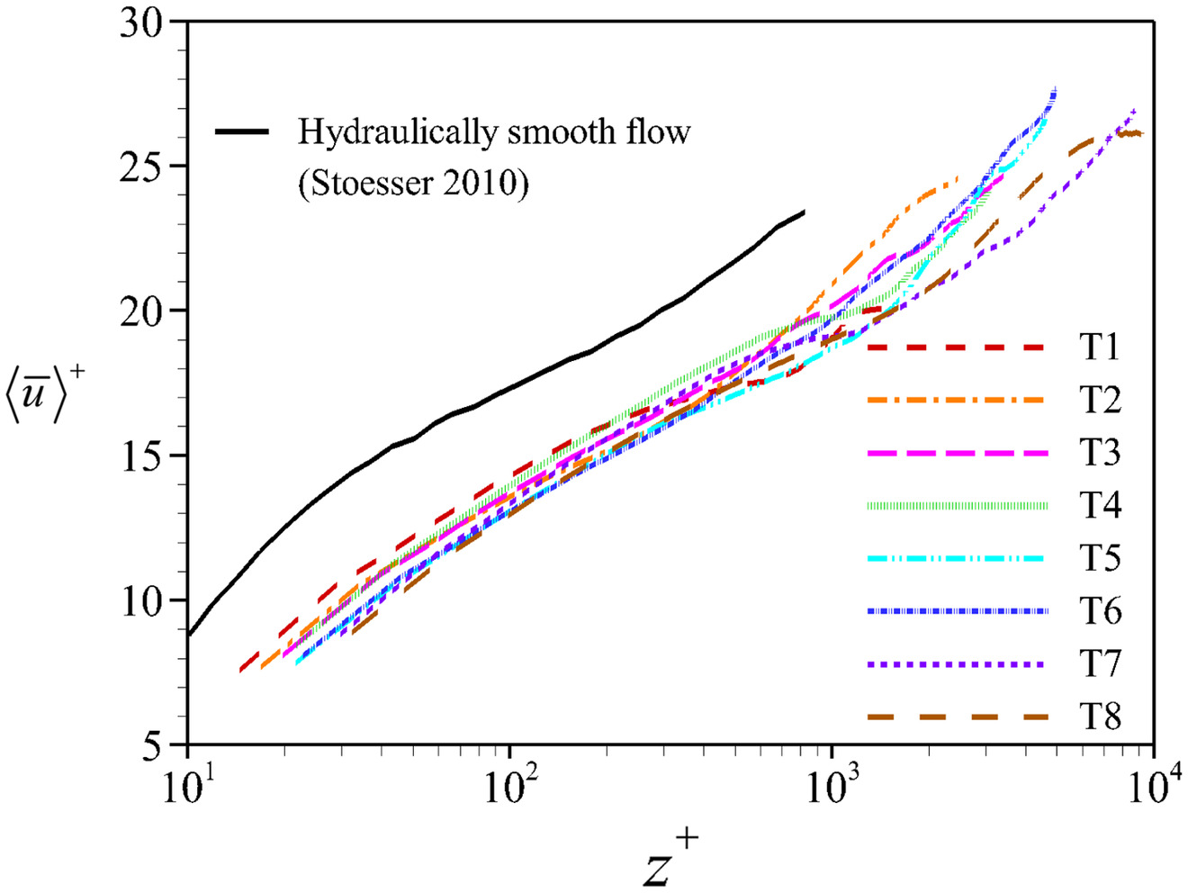
Fig. 2. Dimensionless double-averaged streamwise velocity $⟨ \bar{u} ⟩^{+} (= ⟨ \bar{u} ⟩ / u_{*})$ as a function of dimensionless vertical distance $z^{+} (= z u_{*} / υ)$ for Cases T1–T8 and the velocity profile of a hydraulically smooth flow, after Stoesser (2010).

By definition, the logarithmic law of the wall is (Schlichting 1968)

{⟨ \bar{u} ⟩}^{+} = \frac{1}{κ} \ln \frac{30 z}{k_{s}} = \frac{1}{κ} \ln \frac{30 z^{+}}{k_{s}^{+}} = \frac{1}{κ} \ln z^{+} + \underset{Δ B}{\underset{⏟}{\frac{1}{κ} \ln \frac{30}{k_{s}^{+}}}}

(5)

where

κ

= the von Kármán constant;

k_{s}

= the roughness height; and

k_{s}^{+}

= the roughness Reynolds number, given by

k_{s} u_{*} / υ

. The results of roughness parameters and flow characteristics for Cases T1–T8, derived from Eq. (5), are summarized in Table 3. The values of

κ

and

Δ B

were first determined by fitting the data. Then, the

k_{s}

was derived from

30 / \exp (κ Δ B)

. In Table 3, the values of

k_{s}^{+}

increase from 10 to 34, indicating the flow to be hydraulically transitional for all eight cases. Furthermore, the values of the roughness height

k_{s}

range from 0.54 to 0.97 mm, which are about one to two times the bedload particle size. This suggests that the bedforms are three-dimensional, producing a larger roughness height where the bedload particles accumulate. On the other hand, a smaller roughness height implies that the bed surface is exposed. As a thin layer of spherical bedload particles over the bed was initially set, the roughness height was relatively small after averaging the surface perturbations over the bed. (The characteristics of three-dimensional bedload transport are investigated further in the next section.) In addition, the values of

κ

decrease due to the gradient of the velocity profiles becoming progressively steeper in the sequence of Cases T1–T8.

Table 3. Roughness parameters and flow characteristics for Cases T1–T8

Case	LES shear velocity, $u_{*}$ ( ${ms}^{- 1}$ )	von Kármán constant, $κ$	Translation distance, $Δ B$	Roughness Reynolds number, $k_{s}^{+} = u_{*} k_{s} / υ$	Roughness height, $k_{s}$ (mm)
T1	0.01814	0.400	2.800	10	0.54
T2	0.02114	0.400	1.900	14	0.66
T3	0.02465	0.370	1.358	18	0.74
T4	0.02723	0.360	1.358	18	0.68
T5	0.02714	0.360	0.350	26	0.97
T6	0.02853	0.360	0.250	27	0.96
T7	0.03723	0.345	0.250	28	0.74
T8	0.04041	0.345	$- 0.350$	34	0.84

In addition, in order to validate the bedload transport rate from an integral perspective, the spatially-averaged bedload intensity parameter

Φ

was calculated and analyzed within the simulation domain during the final 1,000 time steps (0.2 s) for Cases T1–T8. The expression is

Φ = \frac{q_{b}}{{(R^{'} g d_{p}^{3})}^{0.5}} = \frac{u_{p} n_{p} V_{p}}{{(R^{'} g d_{p}^{3})}^{0.5}}

(6)

where

u_{p}

= the streamwise particle velocity;

n_{p}

= the number of particles in motion per unit area;

V_{p}

= the volume of the particles; and

R^{'}

= the submerged relative density of particles, given by

(ρ_{s} - ρ) / ρ

.

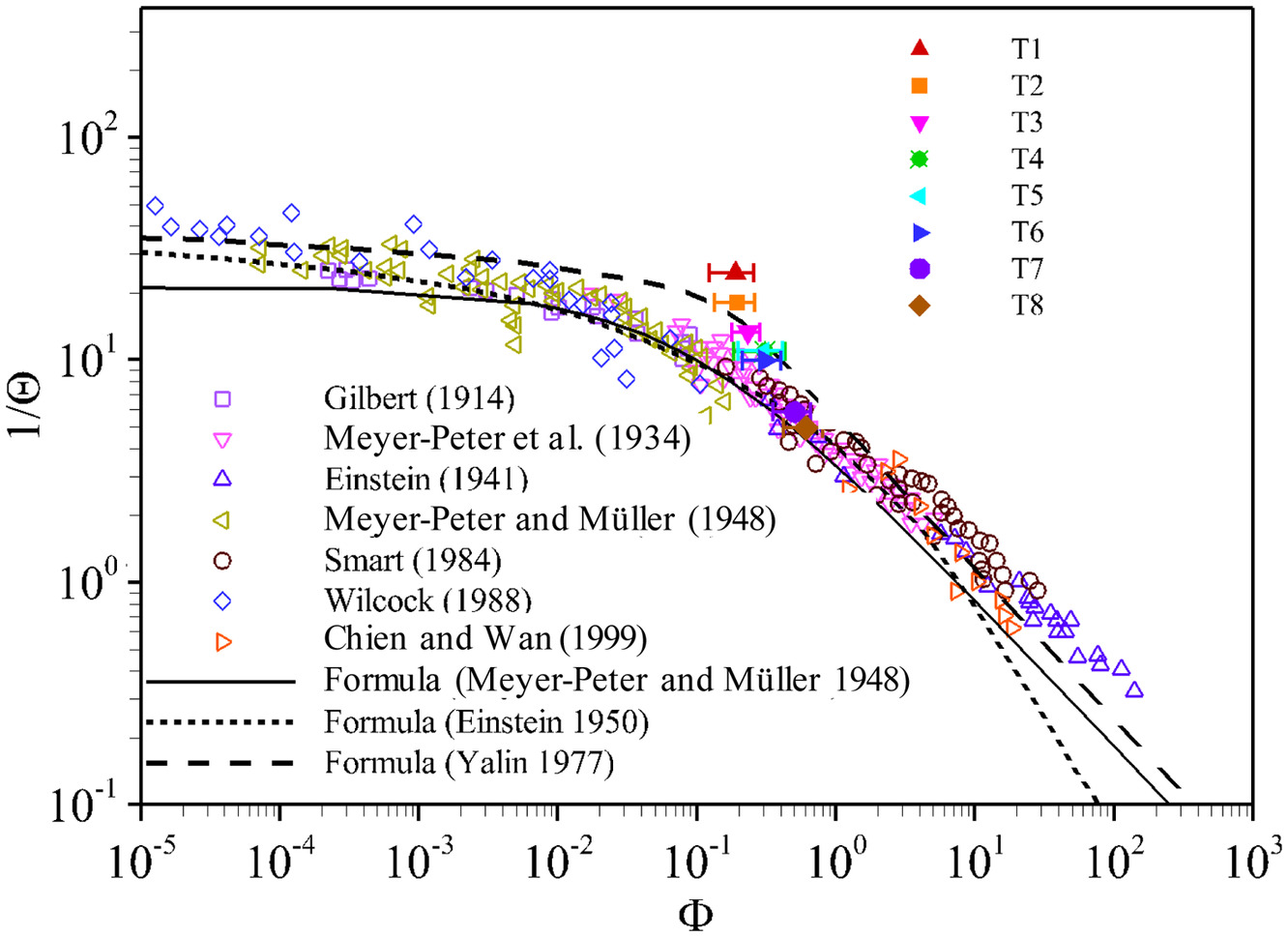
In Fig. 3, the bedload intensity parameter

Φ

versus the flow intensity parameter

1 / Θ

are shown. From Cases T1 to T8, the bedload intensity parameter

Φ

exhibits an increasing trend, as the flow intensity parameter

1 / Θ

decreases. This suggests that the bedload transport capacity declines with the flow intensity parameter

1 / Θ

. A comparison with the previous studies shows that the simulated bedload intensity parameter

Φ

attains a good correlation. This confirms that the present model can adequately account for the driving mechanism in the simulation of bedload transport.

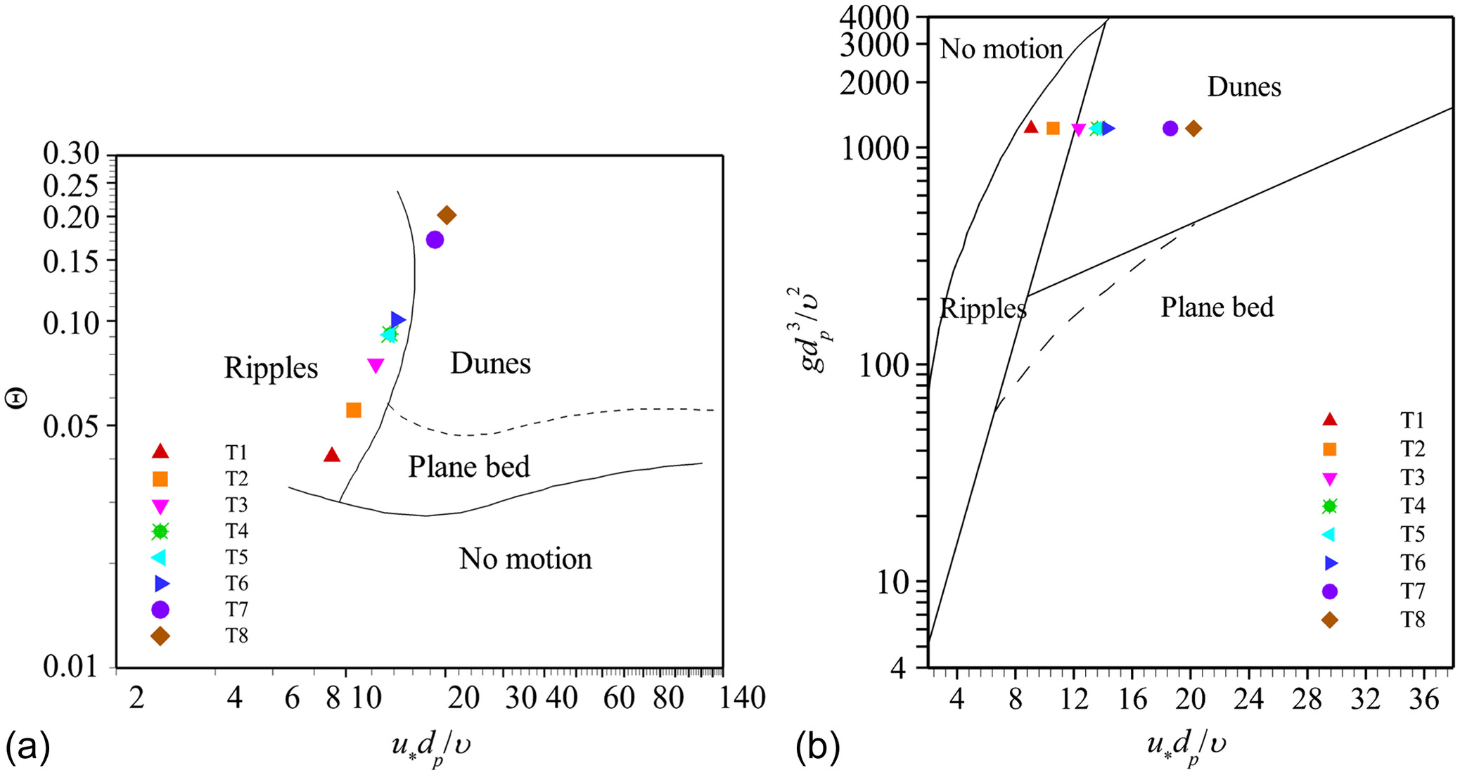
Fig. 3. Bedload intensity parameter $Φ$ versus flow intensity parameter $1 / Θ$ for Cases T1–T8, together with the curves obtained from the classical formulas and the experimental data of various researchers.

The last aspect to validate was the bed patterns for all eight simulations (Cases T1–T8). Their bedform regime diagrams, based on the results of Chabert and Chauvin (1963) and Hill et al. (1971), are plotted in Figs. 4(a and b), respectively. Chabert and Chauvin’s diagram, involving Shields parameter

Θ

versus particle Reynolds number

u_{*} d_{p} / υ

plots, and Hill et al.’s diagram, involving

g d_{p}^{3} / υ^{2}

versus

u_{*} d_{p} / υ

plots, show a good agreement for Cases T1–T3 and T4–T8 (correspond to ripples and dunes, respectively) with the experimental results (Robert and Uhlman 2001; Schindler and Robert 2005). This corroborates that the present simulation results, especially for the integral flow statistics, are quite acceptable.

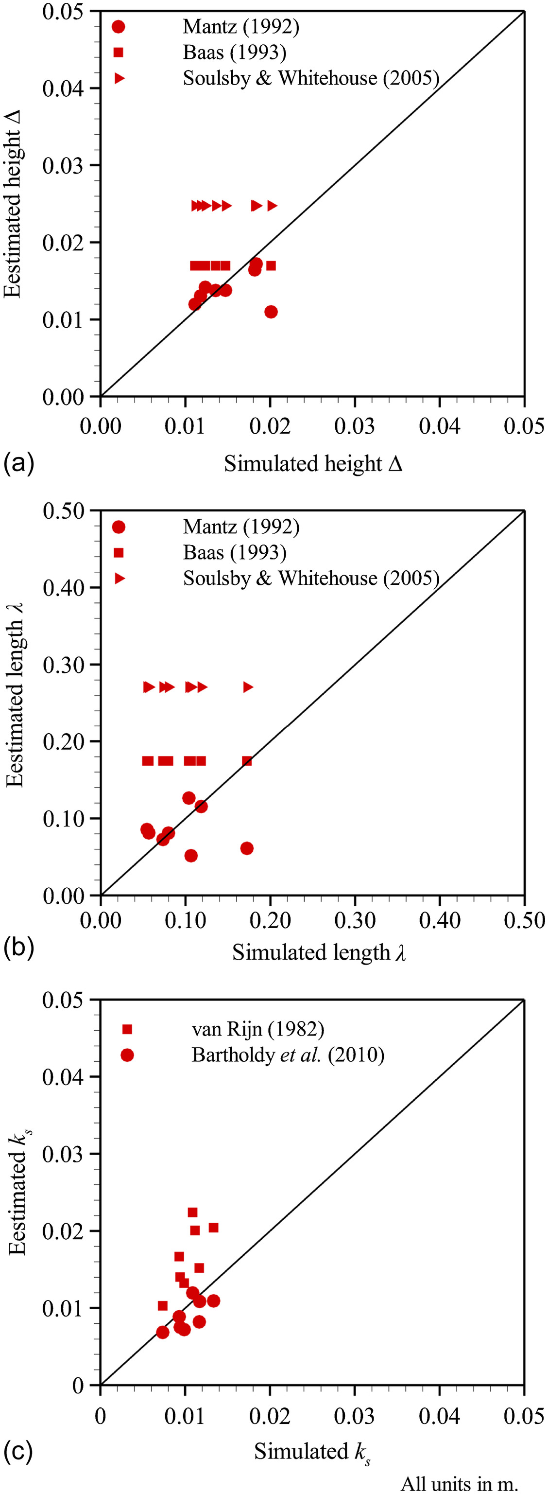
Fig. 4. Bedform regime diagrams for Cases T1–T8: (a) based on the results of Chabert and Chauvin (1963); and (b) based on the results of Hill et al. (1971).

Next, the simulated bedform dimensions, heights

Δ

and lengths

λ

of dunes and ripples, for Cases T1–T8 were plotted and compared with the estimated bedform dimensions obtained from the formulas of various researchers (Mantz 1992; Baas 1993; Soulsby and Whitehouse 2005), as shown in Figs. 5(a and b). This shows that the simulated results of the heights

Δ

and lengths

λ

of the ripples and dunes are consistent with those obtained from the formulas. Furthermore, as the bedload particles are uniform, the roughness height

k_{s}

along the

x

-direction can be considered to be the sum of the particle median size

d_{p}

and the difference between bed and lowest point elevations. Simulated bed roughness

k_{s}

for Cases T1–T8 versus estimated bed roughness obtained from the formulas of van Rijn (1982) and Bartholdy et al. (2010) are represented in Fig. 5(c). The simulated results are in good agreement with those obtained from the formulas, corroborating the efficacy of the model simulation.

Fig. 5. Simulated bedform dimensions for Cases T1–T8 versus estimated bedform dimensions obtained from the formulas of various researchers: (a) heights $Δ$ of dunes and ripples; (b) lengths $λ$ of dunes and ripples; and (c) bed roughness $k_{s}$ .

Result and Discussions

Three-Dimensional Bedload Transport and Bedforms

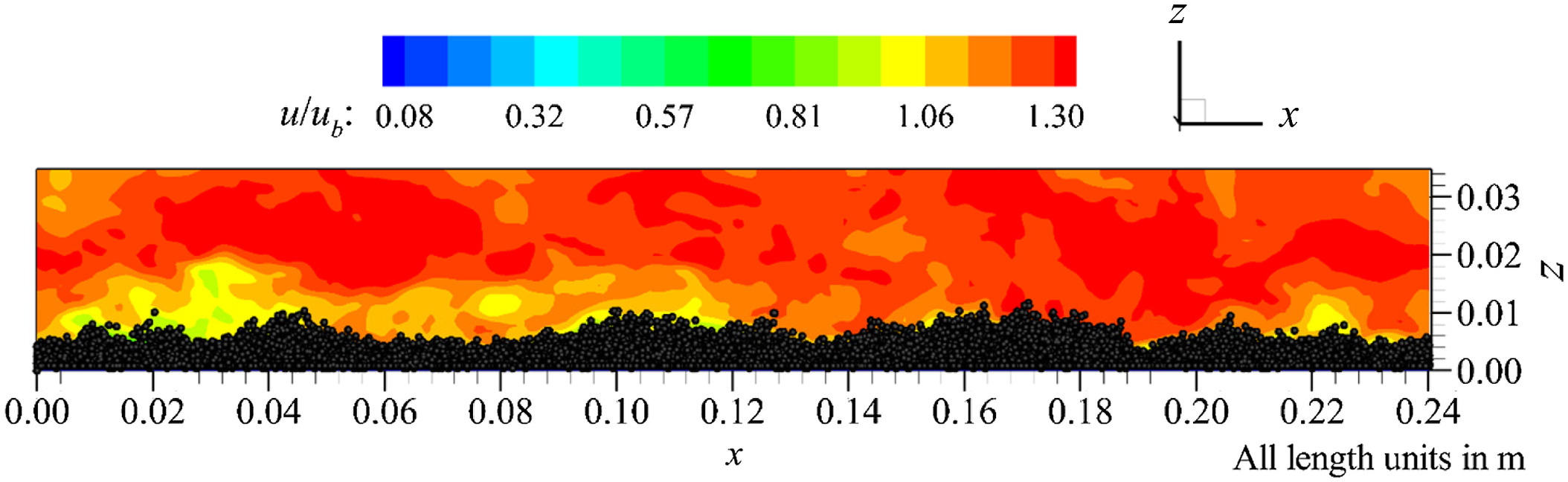
Fig. 6 presents a snapshot of the simulated bedforms for Case T0, including the contours of the dimensionless instantaneous flow velocity

u / u_{b}

on the axis of symmetry of the computational domain. A regular undulant bed formation is evident from the simulation.

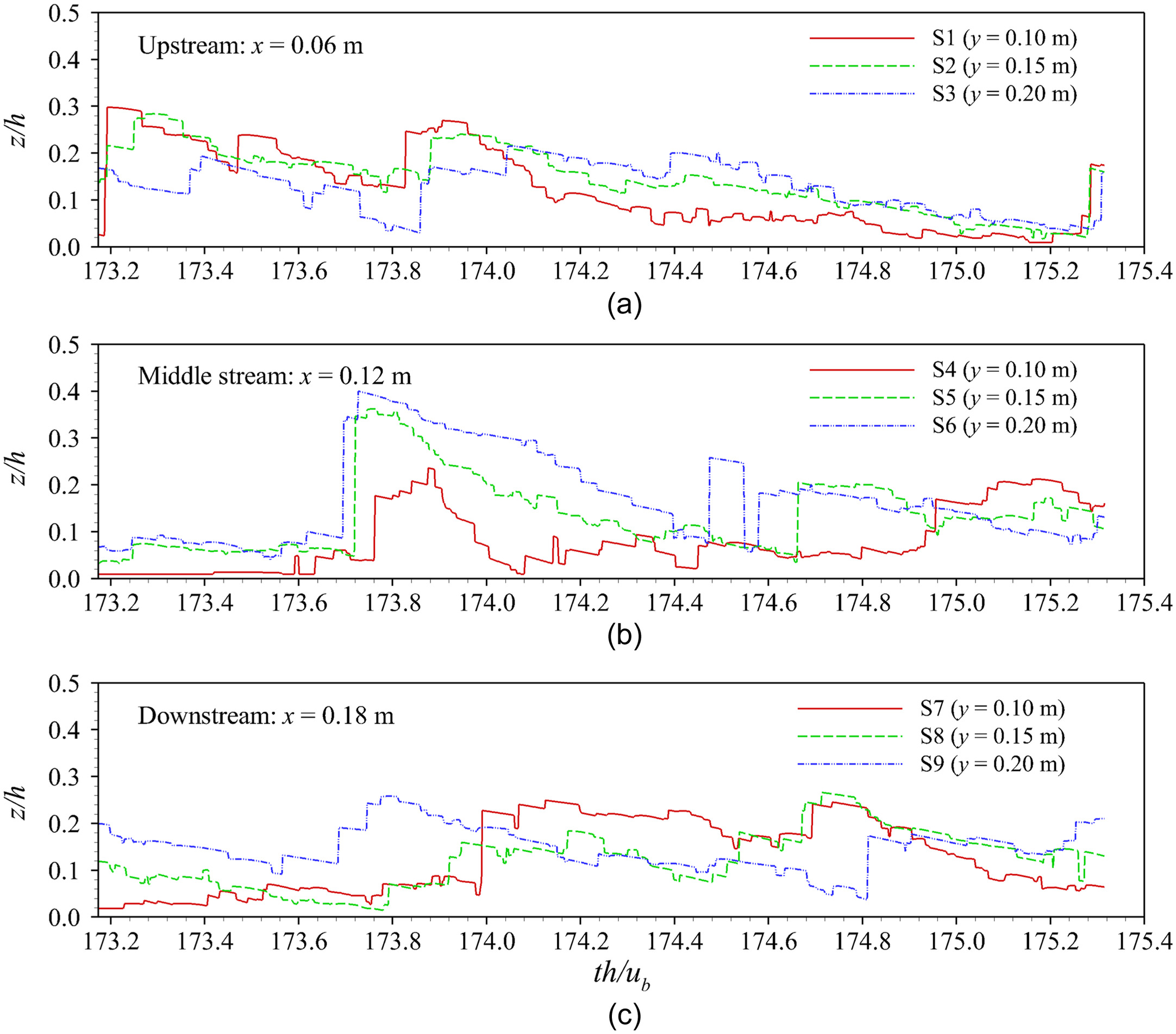
Fig. 6. Snapshot of the simulated bedforms for Case T0 along with the contours of the dimensionless instantaneous flow velocity $u / u_{b}$ on the axis of symmetry of the computational domain.

In order to recognize the process of three-dimensional bedload transport, the bed elevation fluctuations were recorded at nine sample points during a selected time period (1,000 iterations at the end of the simulations) for Case T1. Figs. 7(a–c) show the variations of the dimensionless bed elevation

z / h

with the dimensionless time

t h / u_{b}

on the upstream of the domain (S1–S3) at

x = 0.06 m

, the middle stream (S4–S6) at

x = 0.12 m

, and the downstream (S7–S9) at

x = 0.18 m

for the spanwise distances

y = 0.10

, 0.15, and 0.20 m at each section. They reveal that the bed elevation propagates from the upstream to the downstream with time and also in the spanwise direction. For instance, a comparison of the variations of bed elevations, when

t h / u_{b}

is less than 173.6 in Fig. 7(a) with those when

t h / u_{b}

is from 173.6 to 174.0 in Fig. 7(b), shows that, although the bedload particles transport downstream, the bed elevations propagate from S1–S3 to S4–S6. The peak of S4 is smaller than that of S1, while the peaks of S2 and S3 are greater than those of S5 and S6, respectively. This phenomenon can be explained from the perspective of three-dimensional sediment transport because some bedload particles from S1 are transported to the spanwise direction and downwards to S5 and S6. The movement of the particles is affected by the turbulent flow and, as a result, the particles are transported randomly.

Fig. 7. Variations of the dimensionless bed elevation $z / h$ with the dimensionless time $t h / u_{b}$ for Case T1 at nine sampling locations: (a) upstream S1–S3 at $x = 0.06 m$ ; (b) middle stream S4–S6 at $x = 0.12 m$ ; and (c) downstream S7–S9 at $x = 0.18 m$ . In (a–c), the spanwise distances are $y = 0.10$ , 0.15, and 0.20 m.

Response of Flow Characteristics to Bedload Transport

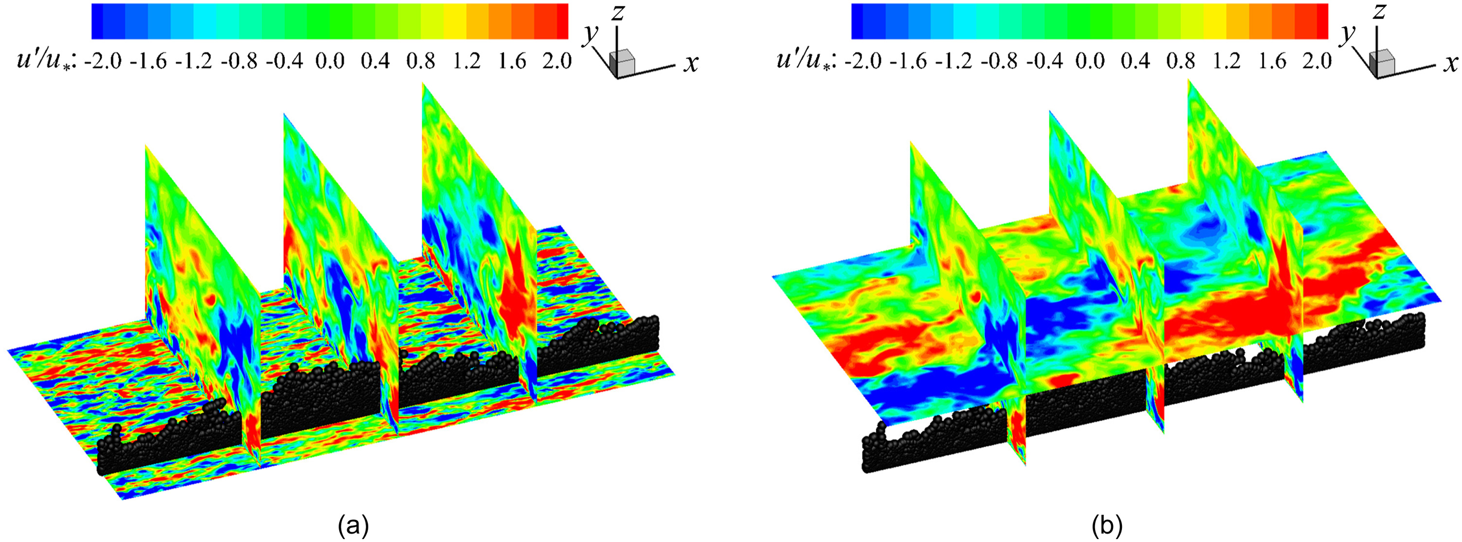
The point is to stress that the three-dimensional bed structure can affect the near-bed flow characteristics. In Figs. 8(a and b), the contours of the dimensionless streamwise velocity fluctuations

u^{'} / u_{*}

are shown on the

y z

-planes at sections

x = 0.06

, 0.12, and 0.18 m including the

x y

-planes at two dimensionless elevations,

z / h = 0

and 0.4, for Case T1. The turbulent coherent structures are clearly apparent as alternative high- and low-speed fluid streaks, which appear almost at a regular spanwise spacing on a

x y

-plane at

z / h = 0

. This demonstrates the near-bed bursting events, which are quasi-periodic processes combining the ejection and sweep events. The ejection involves the arrival of near-bed low-speed fluid streaks to entrain into the mainstream domain, while the sweep is characterized by the arrival of high-speed fluid streaks from the mainstream to rush toward the bed (Dey 2014). However, as the elevation of the plane increases to

z / h = 0.4

, the fluid streaks gradually merge together and the spanwise spacing becomes wider. Over and above, these coherent structures are interrupted by the bed undulations. To be specific, at the stoss-side (upstream) of the ripples, the streamwise velocity fluctuation

u^{'} / u_{*}

is negative (

u^{'} / u_{*} < 0

), which indicates that the near-bed low-speed fluid streaks dominate and entrain into the mainstream domain; while at the leeside (downstream) of the ripples, streamwise velocity fluctuation

u^{'} / u_{*}

is positive (

u^{'} / u_{*} > 0

), which implies that the mainstream high-speed fluid streaks dominate and rush down to the bed.

Fig. 8. Contours of the dimensionless streamwise velocity fluctuations $u^{'} / u_{*}$ on the $y z$ -planes at sections $x = 0.06$ , 0.12, and 0.18 m, including those on the $x y$ -planes at dimensionless elevations of (a) $z / h = 0$ ; and (b) $z / h = 0.4$ for Case T1.

In order to further explore the response of the flow characteristics to the bedload transport, the flow domain on a

x z

-plane, where the bedload particles accumulate, is the main focus here. Cases T1 and T6, which involve relatively low and high flow intensities, respectively, were selected to analyze. The representative planes are located at

y = 0.216

and 1.152 m for Cases T1 and T6, respectively. In Figs. 9(a–f), premultiplied spectra of the streamwise, spanwise, and vertical velocity fluctuations,

k_{x} S_{u^{'} u^{'}}

,

k_{x} S_{v^{'} v^{'}}

, and

k_{x} S_{w^{'} w^{'}}

, respectively, as a function of dimensionless wavelength

λ_{x} / h

at different dimensionless elevations,

z / h = 0.1

, 0.2, and 0.4, for Cases T1 and T6, are compared. Here,

k_{x}

is the wavenumber, which can be derived from the frequency

f

as

k_{x} = 2 π f / ⟨ \bar{u} ⟩

; and

λ_{x}

is the wavelength, which can be calculated as

λ_{x} = ⟨ \bar{u} ⟩ / f

.

Fig. 9. Premultiplied spectra of the streamwise, spanwise, and vertical velocity fluctuations as a function of dimensionless wavelength $λ_{x} / h$ at dimensionless elevations of $z / h = 0.1$ , 0.2, and 0.4: (a) $k_{x} S_{u^{'} u^{'}}$ for Case T1; (b) $k_{x} S_{u^{'} u^{'}}$ for Case T6; (c) $k_{x} S_{v^{'} v^{'}}$ for Case T1; (d) $k_{x} S_{v^{'} v^{'}}$ for Case T6; (e) $k_{x} S_{w^{'} w^{'}}$ for Case T1; and (f) $k_{x} S_{w^{'} w^{'}}$ for Case T6.

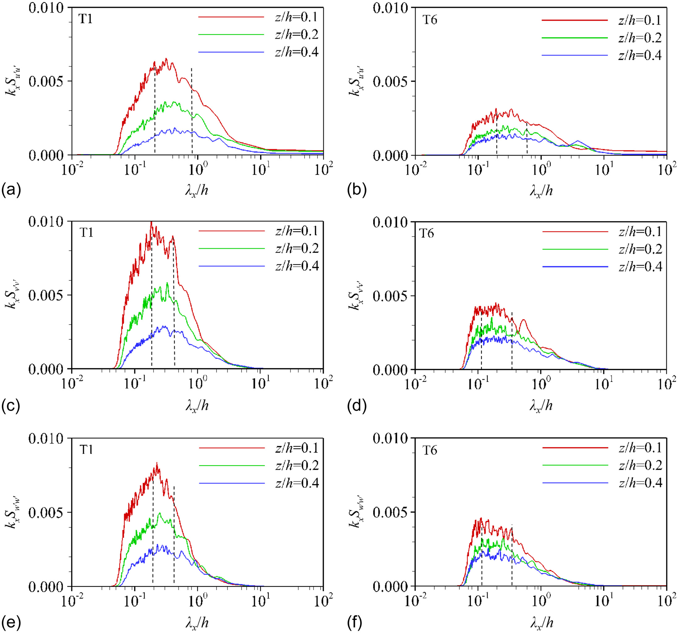
The premultiplied spectrum is a tool to clearly show the distribution of the energy in logarithmic coordinates. A fast Fourier transform is used to calculate the spectrum, the instantaneous spectrum for each instantaneous profile of velocity fluctuations is calculated, and then the averaging is done for all the spectra at each wavenumber

k_{x}

in order to decrease the confidence interval pertaining to each spectral estimate. Figs. 9(a and b), which correspond to the streamwise velocity, show that large-scale coherent structures are generated, and that coherent structures with lengths lying within

0.2 - 0.8 h

(between broken lines) for Case T1 are more prevalent. When the elevation

z / h

is larger, the small-scale region is transformed into the large-scale region and the dimensionless wavelength

λ_{x} / h

increases. This is similar to the spanwise and vertical velocity fluctuations in Figs. 9(c–f), whose fluctuations are more significant in the small-scale region. The coherent structures with lengths lying within

0.18 - 0.45 h

for Case T1 are more prevalent. This shows that the coherent structure dominant scale

λ_{x} / h

for Case T6 in each direction is smaller than that for Case T1. For Case T6, the coherent structures with lengths lying within 0.2–0.6 h for the streamwise velocity fluctuation and 0.12–0.35 h for the spanwise and vertical velocity fluctuations are more prevalent. However, because the flow depth

h

for Case T6 is more than twice that for Case T1, the actual scale is slightly larger for Case T6. In essence, as the turbulence level increases from Case T1 to Case T6, the sizes of the coherent structures near the bed are larger.

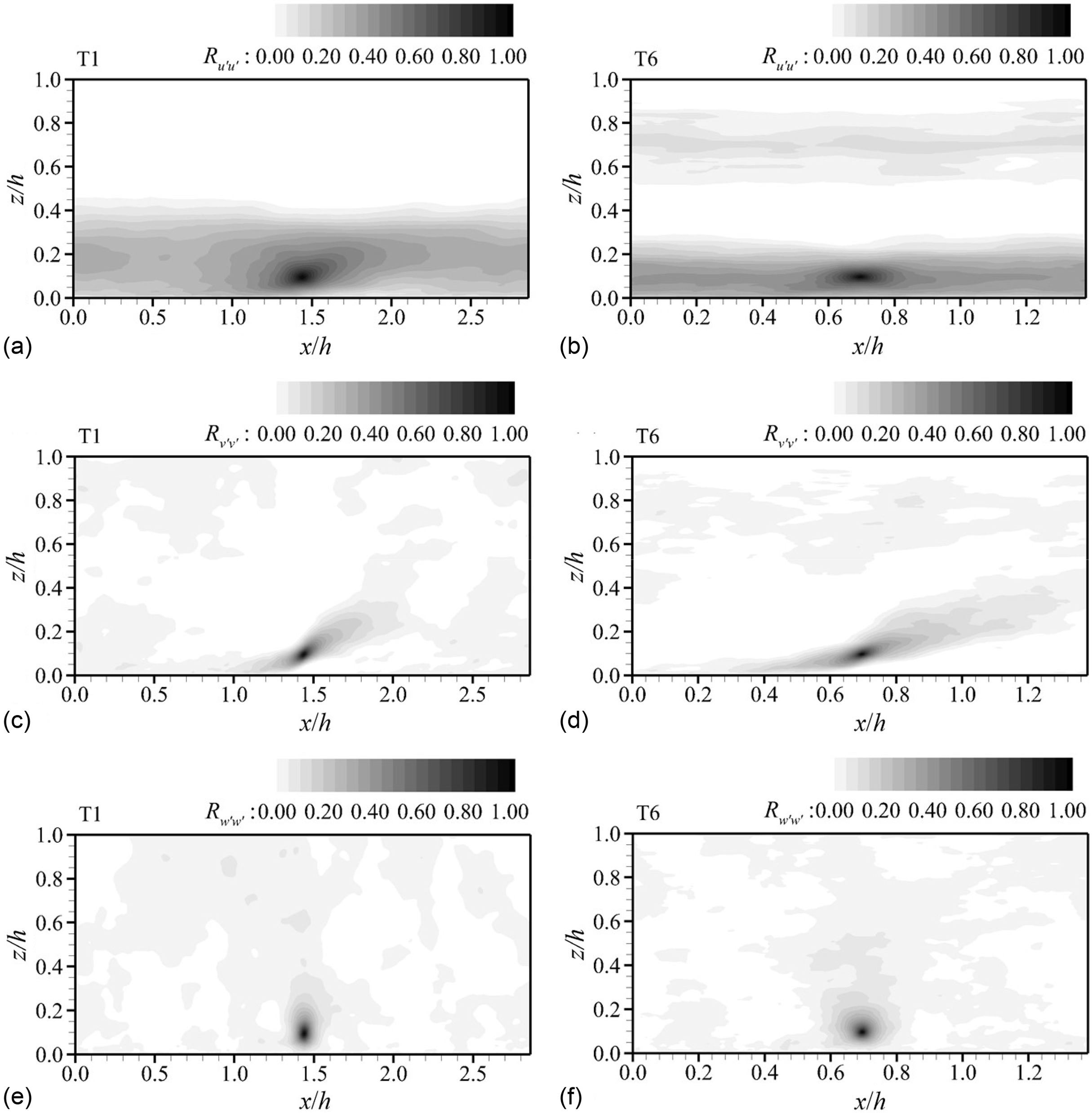
At a given

x z

-plane, the contours of the two-point correlations of the streamwise, spanwise, and vertical velocity fluctuations,

R_{u^{'} u^{'}}

,

R_{v^{'} v^{'}}

, and

R_{w^{'} w^{'}}

, respectively, for Cases T1 and T1 (no particle) are presented in Figs. 10(a–f), and those for Cases T1 and T6 are compared in Figs. 11(a–f). These kinds of plots are effectively used to quantify the length of streaky structures (Kim et al. 1987; Calmet and Magnaudet 1997; Breugem et al. 2006). The two-point correlation functions of streamwise, vertical, and spanwise velocity fluctuations, respectively, can be expressed as:

R_{u^{'} u^{'}} (x_{r}, z_{r}, Δ x, Δ z) = \frac{\sum_{0}^{t} u^{'} (x_{r}, z_{r}, t) u^{'} (x_{r} + Δ x, z_{r} + Δ z, t)}{\sqrt{\sum_{0}^{t} {[u^{'} (x_{r}, z_{r}, t)]}^{2}} \sqrt{\sum_{0}^{t} {[u^{'} (x_{r} + Δ x, z_{r} + Δ z, t)]}^{2}}}

(7)

R_{v^{'} v^{'}} (x_{r}, z_{r}, Δ x, Δ z) = \frac{\sum_{0}^{t} v^{'} (x_{r}, z_{r}, t) v^{'} (x_{r} + Δ x, z_{r} + Δ z, t)}{\sqrt{\sum_{0}^{t} {[v^{'} (x_{r}, z_{r}, t)]}^{2}} \sqrt{\sum_{0}^{t} {[v^{'} (x_{r} + Δ x, z_{r} + Δ z, t)]}^{2}}}

(8)

R_{w^{'} w^{'}} (x_{r}, z_{r}, Δ x, Δ z) = \frac{\sum_{0}^{t} w^{'} (x_{r}, z_{r}, t) w^{'} (x_{r} + Δ x, z_{r} + Δ z, t)}{\sqrt{\sum_{0}^{t} {[w^{'} (x_{r}, z_{r}, t)]}^{2}} \sqrt{\sum_{0}^{t} {[w^{'} (x_{r} + Δ x, z_{r} + Δ z, t)]}^{2}}}

(9)

where

(x_{r}, z_{r})

are the coordinates of the reference point. In Figs. 10(a–f) and 11(a–f), the reference point for each subplot was set at the midpoint of the streamwise length at a dimensionless elevation of

z / h = 0.1

. In the calculation process, a reference point was selected first, and then a long period of velocity fluctuations at each point was taken to perform the foregoing calculation to obtain the two-point correlation functions of each point relative to the reference point.

Fig. 10. Contours of the two-point correlations of the streamwise, spanwise, and vertical velocity fluctuations for Cases T1 and T1 (no particle) (the reference point located at a dimensionless elevation of $z / h = 0.1$ ): (a) $R_{u^{'} u^{'}}$ for Case T1; (b) $R_{u^{'} u^{'}}$ for Case T1 (no particle); (c) $R_{v^{'} v^{'}}$ for Case T1; (d) $R_{v^{'} v^{'}}$ for Case T1 (no particle); (e) $R_{w^{'} w^{'}}$ for Case T1; and (f) $R_{w^{'} w^{'}}$ for Case T1 (no particle).

Fig. 11. Contours of the two-point correlations of the streamwise, spanwise, and vertical velocity fluctuations for Cases T1 and T6 (the reference point located at a dimensionless elevation of $z / h = 0.1$ ): (a) $R_{u^{'} u^{'}}$ for Case T1; (b) $R_{u^{'} u^{'}}$ for Case T6; (c) $R_{v^{'} v^{'}}$ for Case T1; (d) $R_{v^{'} v^{'}}$ for Case T6; (e) $R_{w^{'} w^{'}}$ for Case T1; and (f) $R_{w^{'} w^{'}}$ for Case T6.

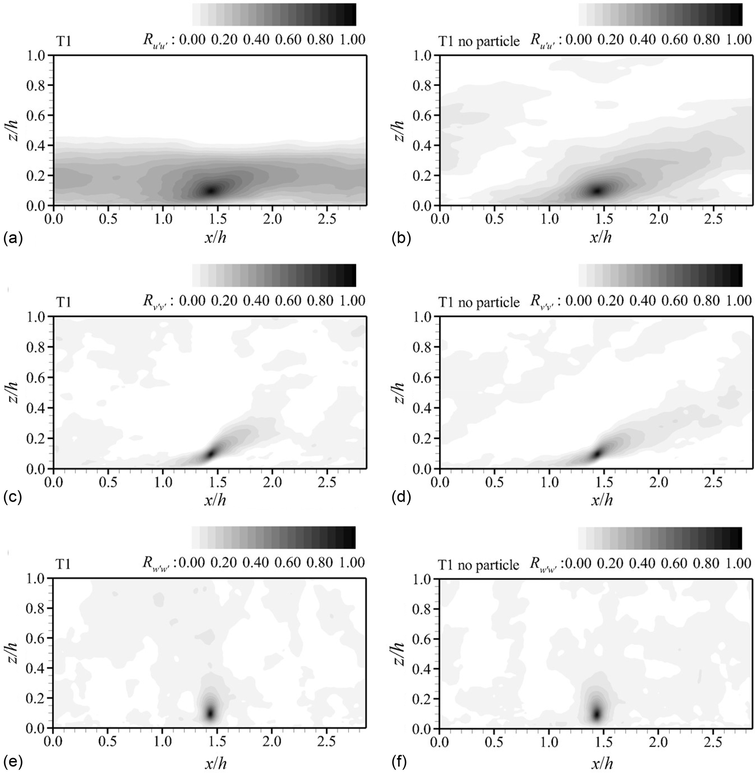
In Fig. 10(a), it is evident that the streamwise velocity fluctuation affects the whole domain length in the

x

-direction. The vertical influence range of

R_{u^{'} u^{'}}

is about

0.45 h

, which is consistent with the results of the premultiplied spectrum discussed previously, and its propagation angle approaches 15°. Variation in the propagation angle is more obvious in Case T1 (no particle), where it increases to 30° diagonally upward. Therefore, the propagation of streamwise velocity fluctuation cannot affect the full streamwise reach of the domain. However, it can affect the flow zone near the free surface. This indicates that the presence of bedload particles reduces the propagation angle of the streamwise velocity fluctuation near the bed, and promotes its propagation along the streamwise direction. The near-bed shear stress increases as well, owing to the bedload particles. It is also apparent that the contours of

R_{v^{'} v^{'}}

and

R_{w^{'} w^{'}}

are similar for Cases T1 and T1 (no particle), in that the spanwise and vertical velocity fluctuations propagate diagonally upward and vertically upward, respectively. The difference can be detected from the influence of the spanwise velocity fluctuation toward the free surface, which is larger for Case T1 (no particle) than for Case T1.

Comparing the contours between Cases T1 and T6 in Figs. 11(a–f), the propagation angles of the velocity fluctuations are quite different. For instance, the propagation angle of

R_{v^{'} v^{'}}

for Case T6 is smaller (nearly 30° diagonally upwards) than for Case T1 (nearly 45° diagonally upwards). Although the affected dimensionless length in the vertical direction seems to be smaller than Case T1, the actual scale is larger for Case T6, because the flow depth

h

for Case T6 is more than twice that for Case T1.

In order to explore the velocity fluctuations, which reflect the coherent structures and quantify their contributions to the Reynolds shear stress, quadrant analysis (Lu and Willmarth 1973) is applied here. Figs. 12(a–f) show the quadrant analysis of the probability density functions of dimensionless velocity fluctuations

u^{'} / u_{*}

and

w^{'} / u_{*}

at dimensionless elevations of

z / h = 0.1

, 0.2, and 0.4 for Cases T1 and T6, respectively. The first quadrant corresponds to the outward interaction

(u^{'} > 0, w^{'} > 0)

, the second quadrant to the ejection

(u^{'} < 0, w^{'} > 0)

, the third quadrant to the inward interaction

(u^{'} < 0, w^{'} < 0)

, and the fourth quadrant to the sweep

(u^{'} > 0, w^{'} < 0)

. The ejection transports a low momentum fluid upwards away from the bed, while the sweep transports a high momentum fluid downward toward the bed.

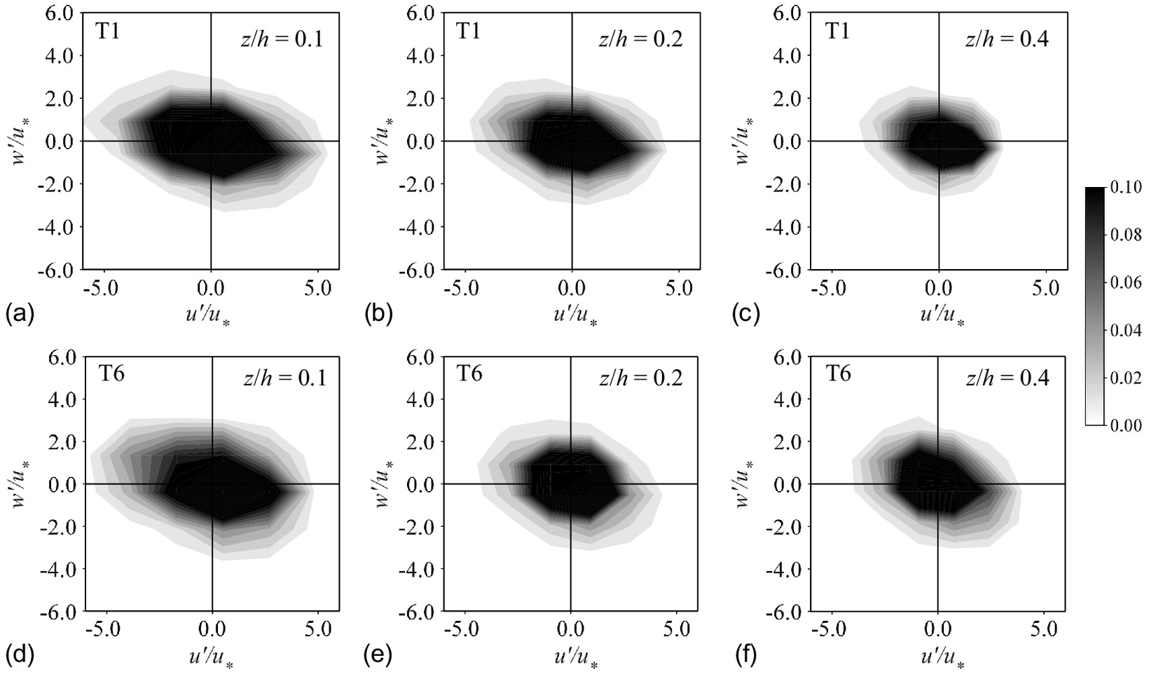
Fig. 12. Quadrant plots of the probability density functions of dimensionless velocity fluctuations $u^{'} / u_{*}$ and $w^{'} / u_{*}$ at dimensionless elevations of (a) $z / h = 0.1$ for Case T1; (b) $z / h = 0.2$ for Case T1; (c) $z / h = 0.4$ for Case T1; (d) $z / h = 0.1$ for Case T6; (e) $z / h = 0.2$ for Case T6; and (f) $z / h = 0.4$ for Case T6.

In Figs. 12(a–c), the 45° oblique oval-shaped plots reflect that the proportions of the four quadrants are not equal. Both the ejection and sweep are dominant for Case T1 at

z / h = 0.1

and the ejection phenomenon accounts for a larger proportion. As the elevation increases, the contribution from the ejection weakens while the sweep strengthens [Fig. 12(c)]. It is obvious that the region with a negative

u^{'} w^{'}

, that is, where the ejection–sweep phenomenon occurs, is more significant near the bed, where the bedload particles transport actively. The presence of bedload particles increases the bursting events in the flow and causes the mixing of high- and low-speed fluids to intensify. For Case T6 in Figs. 12(d–f), although the ejection–sweep phenomenon is dominant near the bed surface at

z / h = 0.1

, the dominance is weaker than that for Case T1 due to an increase in flow intensity. This phenomenon disappears quickly at

z / h = 0.2

, and the contributions from the four quadrants tend to be equal.

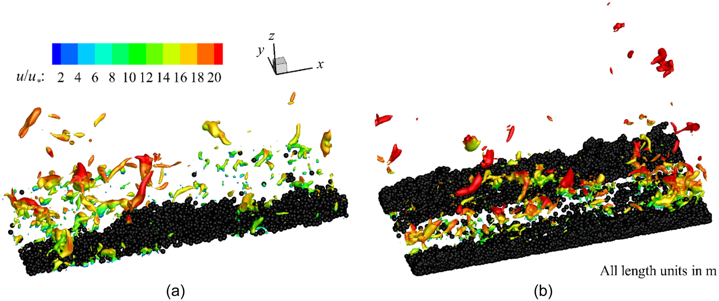
In order to represent the turbulent structures expressively, the instantaneous flow structures visualized with the isosurfaces of dimensionless pressure fluctuation

- 2 p^{'} / ρ u_{*}^{2} = 9.5

for Cases T1 and T6 are depicted in Figs. 13(a and b). They are contoured with the dimensionless instantaneous streamwise velocity

u / u_{*}

. The kolk–boil vortices in the form of the streamwise elongated structures and the hairpin vortices are evident over the trough of the bedforms.

Fig. 13. Instantaneous flow structures visualized with the isosurface of dimensionless pressure fluctuation $- 2 p^{'} / ρ u_{*}^{2} = 9.5$ (contours of the dimensionless instantaneous streamwise velocity $u / u_{*}$ ) with bed particles for (a) Case T1; and (b) Case T6.

Relationship between Vorticity and Bedload Transport Rate

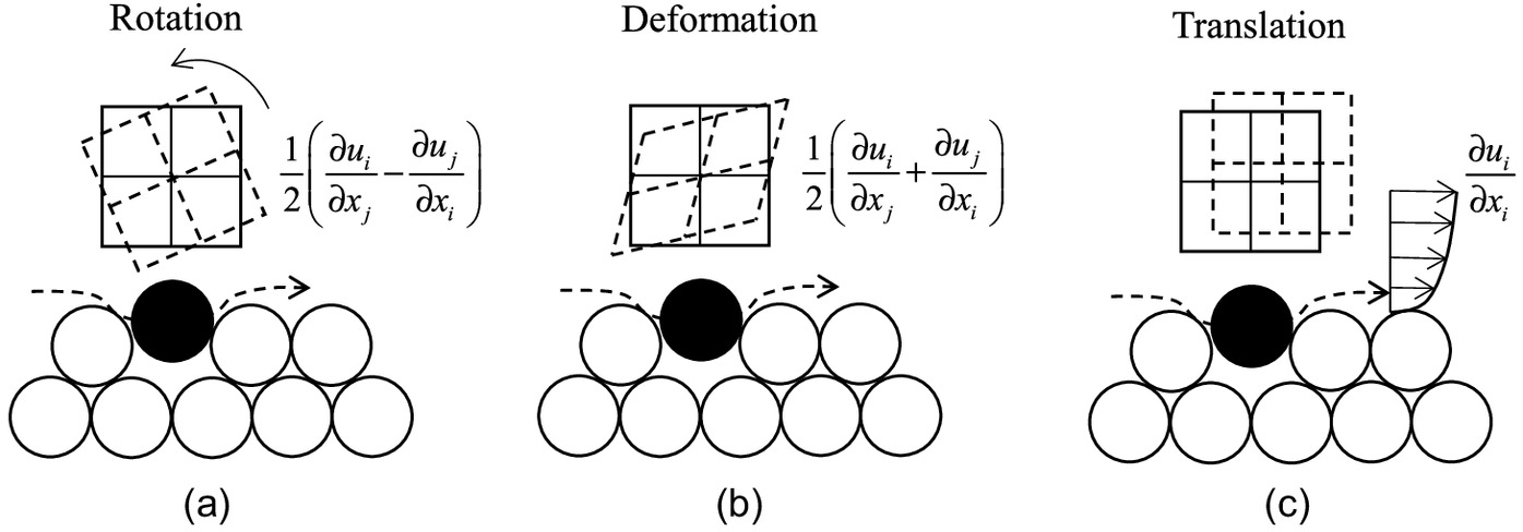
In order to examine the relationship between vorticity and bedload transport, the

Q

criterion that accounts for the strain rate and the vorticity tensors can be applied for the quantification as follows:

Q = \frac{1}{2} ({| Ω_{i j} |}^{2} - {| S_{i j} |}^{2})

(10)

where

S_{i j}

= the strain rate tensor; and

Ω_{i j}

= the vorticity tensor. They can be obtained from the following expressions:

S_{i j} = \frac{1}{2} (\frac{\partial u_{i}}{\partial x_{j}} + \frac{\partial u_{j}}{\partial x_{i}})

(11)

Ω_{i j} = \frac{1}{2} (\frac{\partial u_{i}}{\partial x_{j}} - \frac{\partial u_{j}}{\partial x_{i}})

(12)

Thus, in a three-dimensional simulation, the

Q

value can be displayed as follows:

Q = \underset{\binom{Fluid rotation term}{F 1}}{\underset{⏟}{(Ω_{12}^{2} + Ω_{13}^{2} + Ω_{23}^{2})}} - \underset{\binom{Fluid deformation term}{F 2}}{\underset{⏟}{(S_{12}^{2} + S_{13}^{2} + S_{23}^{2})}} - \underset{\binom{Fluid translation term}{F 3}}{\underset{⏟}{0.5 (S_{11}^{2} + S_{22}^{2} + S_{33}^{2})}}

(13)

The three separative terms of the fluid elements represent the intensities of three kinds of fluid vortex motions: fluid rotation, deformation, and translation, denoted by

F 1

,

F 2

, and

F 3

, respectively.

From the definition of fluid shear stress

τ_{0}

, which initiates the sediment motion, it is the function of the squared shear velocity

u_{*}

and is proportional to the velocity gradient

\partial u_{i} / \partial x_{j}

, called the shear strain rate:

τ_{0} = ρ u_{*}^{2} = ρ υ \frac{\partial u_{i}}{\partial x_{j}}

(14)

Hence, the shear strain rate,

\partial u_{i} / \partial x_{j} = u_{*}^{2} / υ

, can be derived from the bed shear stress or the shear velocity related to the strain rate and vorticity tensors, linking to the fluid rotation, deformation, and translation terms, as follows:

\frac{u_{*}^{2}}{υ} \sim (\begin{array}{c} Ω_{12} & Ω_{13} & Ω_{23} \\ S_{12} & S_{13} & S_{23} \\ S_{22} & S_{11} & S_{33} \end{array})

(15)

This implies that the shear stress that affects the bedload transportation is essentially a combination of forces caused by the rotation, deformation, and translation of a fluid vortex. Figs. 14(a–c) provide the schematic representation of the related mechanism.

Fig. 14. Schematic illustrations of the three mechanisms of a fluid vortex acting on the bedload particles: (a) rotation; (b) deformation; and (c) translation.

By collecting and averaging the samples around the bedload particles, the bedload intensity parameters

Φ

as a function of the separative terms of the fluid elements for Cases T1–T8 are presented in Figs. 15(a–c). It can been seen that the fluid deformation term

F 2

is the same as the fluid rotation term

F 1

, and that they each have a similar trend as the fluid translation term

F 3

.

Fig. 15. Bedload intensity parameter $Φ$ as a function of separative terms of fluid elements and shear strain rate for Cases T1–T8: (a) $Φ$ versus fluid rotation term $F 1$ ; (b) $Φ$ versus fluid deformation term $F 2$ ; (c) $Φ$ versus fluid translation term $F 3$ ; and (d) $Φ$ versus shear strain rate $u_{*}^{2} / υ$ .

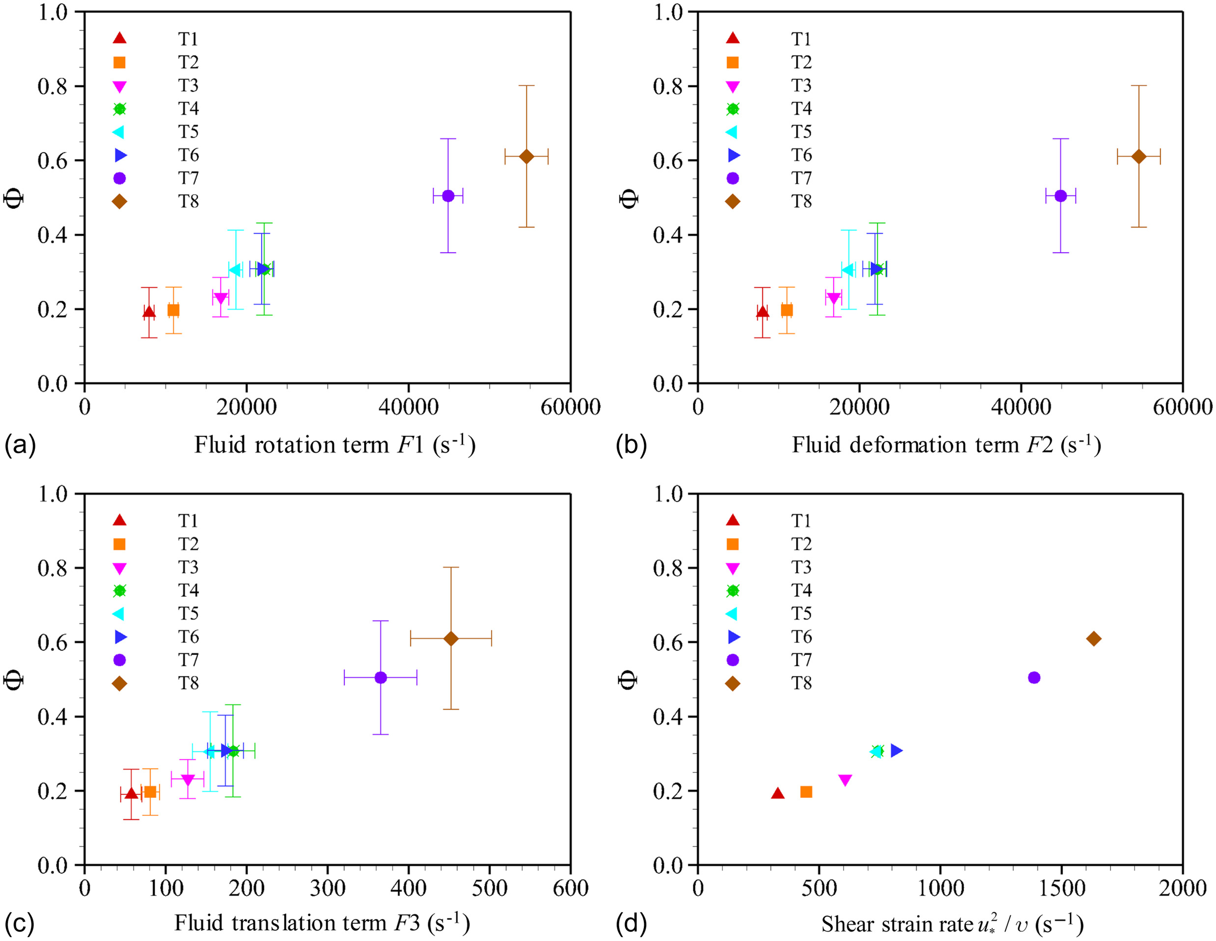
As the flow intensity increases, the fluid rotation term

F 1

, deformation term

F 2

, and translation term

F 3

increase. In turn, the bedload intensity parameter

Φ

increases as all three terms increase, and appears to satisfy a linearly increasing relationship.

In general, the bedload intensity parameter

Φ

satisfies the following relation (Dey 2014):

Φ = K {(Θ - Θ_{c})}^{m}

(16)

where

Θ

and

Θ_{c}

are the Shields parameter and critical Shields parameter for bed particle motion, respectively;

K

is a coefficient; and

m

is an exponent. The coefficient

K

has variable values and the typical values for the exponent

m

are 0.5, 1, and 1.5.

As

Θ

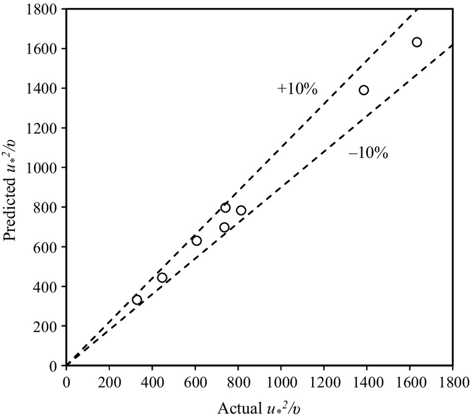
is the dimensionless form of

τ_{0}

, it relates to the shear strain rate

u_{*}^{2} / υ

as well. In Fig. 15(d), the relationship between bedload intensity parameter

Φ

and

u_{*}^{2} / υ

is represented, which also meets the relationship in Eq. (16). Therefore, as long as

u_{*}^{2} / υ

can be accurately determined, the bedload intensity parameter

Φ

can be effectively predicted. Fitting

u_{*}^{2} / υ

and the fluid rotation, deformation, and translation terms, the following expression is obtained:

\frac{u_{*}^{2}}{υ} = \max [0.011 (F 1 + F 2) + 129 \ln (F 3) - 368, 0]

(17)

The

R^{2}

of this expression was calculated as 0.996. Fig. 16 shows the comparisons between the predicted values of

u_{*}^{2} / υ

obtained from Eq. (17) and the actual values obtained from the eight Cases T1–T8. The largest deviation was observed to be about

\pm 10 %

. Therefore, it can be argued that Eq. (17) is adequate to estimate

u_{*}^{2} / υ

. In Eq. (17), an increase in fluid translation term

F 3

influences the final value of the bed friction velocity

u_{*}

more than either the fluid rotation term

F 1

or the deformation term

F 2

, both of which contribute the same. From Fig. 15 in association with Eq. (13), it is evident that the three terms

F 1

,

F 2

, and

F 3

are interrelated. Given these arguments, the three terms are seen to be equally important for the bed friction velocity. Furthermore, as long as the statistics of the law of fluid vortex motion have been obtained, the

u_{*}^{2} / υ

can be accurately predicted as to the bedload intensity parameter

Φ

, as a modification of the Meyer-Peter and Müller (1948) formula

Φ = 8 {\frac{ρ υ}{g R^{'} d_{p}} \max [0.011 (F 1 + F 2) + 129 \ln (F 3) - 368, 0] - Θ_{c}}^{1.5}

(18)

Fig. 16. Comparison between predicted and actual $u_{*}^{2} / υ$ for Cases T1–T8. Broken lines represent errors of $\pm 10 %$ .

It is pertinent to mention the usefulness of Eq. (17) in computing the bedload intensity parameter given by Eq. (18). Eq. (17) involves the fluid rotation, deformation, and translation terms in transporting the sediment particles as a bedload. No existing empirical formulas or analytical (deterministic or probabilistic) methods take them into account in computing bedload. Therefore, the present formula is considered to be comprehensive regarding the role of fluid vortex motions on bedload transport.

Conclusions

In this study, a LES was used to simulate the turbulent flow, the NS equations were applied as the governing equations for the fluid, and the Eulerian method was employed to solve the NS equations. With regard to bedload particle dynamics, the Lagrangian point-particle model was applied to track the trajectories of the particles and to determine the forces exerted by the flow on them. Particle–wall collisions were considered, and the time-saving model of particle–particle collisions was evolved. Nine cases of simulations were carried out along the lines of previous experiments for bedform regimes, namely ripples and dunes.

In this study, the sediment transport is three-dimensional. The bedload transport intensities and the dimensions of bedforms for all the cases agree well with the results obtained from the classical formulas. From an examination of the fluid motion near the accumulated bedload particles, kolk–boil vortices in the form of the streamwise elongated structures and the hairpin vortices form over the trough of the bedforms. Turbulent coherent structures in the form of high- and low-speed fluid streaks near the bed are also affected by the bedforms. The near-bed low-speed fluid streaks entrain into the mainstream domain over the stoss-side of ripples and the high-speed fluid streaks from the mainstream rush toward the bed over the leeside of ripples. The ejection and sweep events prevail near the bed, where the bedload particles transport. However, the phenomenon disappears as the flow intensity increases. The presence of bedload particles also modifies the propagation angle and the range of velocity fluctuations, especially in the streamwise direction.

To quantify the fluid vortex motion, the decomposition parts of the fluid rotation, deformation, and translation terms, which demonstrate three kinds of vortical motions, were calculated separately. It was found that they increase linearly with the bedload intensity parameter as the flow intensity parameter increases. Finally, an improved formula for bedload intensity parameters relating the fluid rotation, deformation, and translation terms was obtained. This suggests that, as long as these three terms are obtained accurately (which is a scope of future research), the bed shear stress and bedload transport rate can be effectively predicted.

Notation

The following symbols are used in this paper:

$C_{m}$: added mass coefficient;
$d_{p}$: nominal particle diameter;
$F 1$ , $F 2$ , $F 3$: fluid rotation, deformation, and translation terms, respectively;
$F_{p, i}$: total force acting on a particle in the $i$ -direction;
$F r$: flow Froude number;
$f$: frequency;
$f_{p, i}$: total force per unit volume exerted by the particles on the fluid in the $i$ -direction;
$g$: gravitational acceleration;
$h$: flow depth;
$I_{p}$: moment of inertia of a particle;
$K$: coefficient;
$k_{s}$: roughness height;
$k_{s}^{+}$: roughness Reynolds number, given by $k_{s} u_{*} / υ$ ;
$k_{x}$: wavenumber;
$m$: exponent;
$m_{p}$: total mass of a particle including added mass;
$N_{p, i}$: torque about the $i$ -axis;
$n_{p}$: number of particles in motion per unit area;
$n_{x}$ , $n_{y}$ , $n_{z}$: numbers of computational cells in the $x$ -, $y$ -, and $z$ -directions, respectively;
$p$: instantaneous pressure;
$p^{'}$: pressure fluctuation;
$Q$: criterion accounting for the strain rate and vorticity tensors;
$R$: hydraulic radius;
$R^{'}$: submerged relative density of particles, given by $(ρ_{s} - ρ) / ρ$ ;
$R e$: flow Reynolds number;
$R e_{τ}$: friction Reynolds number;
$R_{u^{'} u^{'}}$ , $R_{v^{'} v^{'}}$ , $R_{w^{'} w^{'}}$: two-point correlations of streamwise, vertical, and spanwise velocity fluctuations, respectively;
$S_{i j}$: strain-rate tensor, given by $(\partial u_{i} / \partial x_{j} + \partial u_{j} / \partial x_{i}) / 2$ ;
$S_{u^{'} u^{'}}$ , $S_{v^{'} v^{'}}$ , $S_{w^{'} w^{'}}$: spectral density functions of streamwise, spanwise, and vertical velocity fluctuations, respectively;
$t$: time;
$⟨ ū ⟩$: spatially-averaged $ū$ over the fluid surface (domain) at a vertical distance $z$ ;
$ū$: time-averaged streamwise velocity at a vertical distance $z$ ;
$u^{'}$ , $v^{'}$ , $w^{'}$: fluctuations of streamwise, spanwise, and vertical velocities with respective to their respective time-averaged values;
$u_{*}$: shear velocity;
$u_{i}$ , $u_{j}$: flow velocities in the $i$ - and $j$ -directions, respectively;
$u_{p}$: streamwise particle velocity;
$u_{p, i}$: particle velocity in the $i$ -direction;
$u_{0}$: area-averaged flow velocity;
$V_{p}$: volume of particles;
$x$ , $y$ , $z$: streamwise, spanwise, and vertical distances, respectively;
$x_{i}$ , $x_{j}$: spatial variables in the $i$ - and $j$ -directions, respectively;
$x_{r}$ , $z_{r}$: coordinates of the reference point;
$z^{+}$: dimensionless vertical distance;
$Δ x$ , $Δ y$ , $Δ z$: grid spacings in the $x$ -, $y$ -, and $z$ -directions, respectively;
$Δ x^{+}$ , $Δ y^{+}$ , $Δ z^{+}$: dimensionless grid spacings in the $x$ -, $y$ -, and $z$ -direction, respectively;
$Θ$: Shields parameter, given by $u_{*}^{2} / g R^{'} d_{p}$ ;
$Θ_{c}$: critical Shields parameter for bed particle motion;
$κ$: von Kármán constant;
$λ_{x}$: wavelength;
$ρ$: fluid mass density;
$ρ_{s}$: particle mass density;
$τ_{0}$: bed shear stress induced by the flow;
$τ_{c}$: threshold bed shear stress for the initiation of sediment particle motion;
$τ_{i j}$: sub-grid stress tensor, given by $2 υ_{t} S_{i j}$ ;
$υ$: fluid kinematic viscosity;
$υ_{t}$: sub-grid stress viscosity;
$Φ$: bedload intensity parameter;
$Ω_{i j}$: vorticity tensor; and
$ω_{p, i}$: particle angular velocity about the $i$ -axis.

Data Availability Statement

All data that support the findings of this study can be downloaded from the Zenodo website (https://doi.org/10.5281/zenodo.6367481). The code package is available on the GitHub website https://github.com/OuroPablo/Hydro3D.

Acknowledgments

This investigation was supported by the National Natural Science Foundation of China (Nos. 12172196 and U2040214), National Key Research and Development Project (2022YFC3201800), and the 111 Project (B18031).

References

Baas, J. H. 1993. Dimensional analysis of current ripples in recent and ancient depositional environments (Geologica ultraiectina). Utrecht, Netherlands: Faculteit Aardwetenschappen Der Rijksuniversi.

Google Scholar

Bagherimiyab, F., and U. Lemmin. 2012. “Fine sediment dynamics in unsteady open-channel flow studied with acoustic and optical systems.” Continental Shelf Res. 46 (Sep): 2–15. https://doi.org/10.1016/j.csr.2012.04.014.

Google Scholar

Bai, J., H. Fang, and T. Stoesser. 2013. “Transport and deposition of fine sediment in open channels with different aspect ratios.” Earth Surf. Processes Landforms 38 (6): 591–600. https://doi.org/10.1002/esp.3304.

Google Scholar

Balachandar, S. 2009. “A scaling analysis for point-particle approaches to turbulent multiphase flows.” Int. J. Multiphase Flow 35 (9): 801–810. https://doi.org/10.1016/j.ijmultiphaseflow.2009.02.013.

Google Scholar

Bartholdy, J., B. W. Flemming, V. B. Ernstsen, C. Winter, and A. Bartholom ä. 2010. “Hydraulic roughness over simple subaqueous dunes.” Geo-Mar. Lett. 30 (1): 63–76. https://doi.org/10.1007/s00367-009-0153-7.

Google Scholar

Bradley, R. W., and J. G. Venditti. 2017. “Reevaluating dune scaling relations.” Earth Sci. Rev. 165 (Feb): 356–376. https://doi.org/10.1016/j.earscirev.2016.11.004.

Google Scholar

Breugem, W. P., B. J. Boersma, and R. E. Uittenbogaard. 2006. “The influence of wall permeability on turbulent channel flow.” J. Fluid Mech. 562 (Sep): 35–72. https://doi.org/10.1017/S0022112006000887.

Google Scholar

Bui, M. D., and P. Rutschmann. 2010. “Numerical modelling of non-equilibrium graded sediment transport in a curved open channel.” Comput. Geosci. 36 (6): 792–800. https://doi.org/10.1016/j.cageo.2009.12.003.

Google Scholar

Bui, V. H., M. D. Bui, and P. Rutschmann. 2019. “Advanced numerical modeling of sediment transport in gravel-bed rivers.” Water 11 (3): 550. https://doi.org/10.3390/w11030550.

Google Scholar

Calmet, I., and J. Magnaudet. 1997. “Large-eddy simulation of high-Schmidt number mass transfer in a turbulent channel flow.” Phys. Fluids 9 (2): 438–455. https://doi.org/10.1063/1.869138.

Google Scholar

Cao, Z. 1997. “Turbulent bursting-based sediment entrainment function.” J. Hydraul. Eng. 123 (3): 233–236. https://doi.org/10.1061/(ASCE)0733-9429(1997)123:3(233).

Google Scholar

Cevheri, M., R. McSherry, and T. Stoesser. 2016. “A local mesh refinement approach for large-eddy simulations of turbulent flows.” Int. J. Numer. Methods Fluids 82 (5): 261–285. https://doi.org/10.1002/fld.4217.

Google Scholar

Chabert, J., and T. L. Chauvin. 1963. “Formation des dunes et de rides dans les modeles fluviaux.” Bull. Du Centre de Recherches et d’Essais de Chatou 4 (Jun): 31–52.

Google Scholar

Clifford, N. J., J. McClatchey, and J. R. French. 1991. “Measurements of turbulence in the benthic boundary layer over a gravel bed and comparison between acoustic measurements and predictions of the bedload transport of marine gravels.” Sedimentology 38 (1): 161–166. https://doi.org/10.1111/j.1365-3091.1991.tb01863.x.

Google Scholar

Dey, S. 2014. Fluvial hydrodynamics: Hydrodynamic and sediment transport phenomena. Berlin: Springer.

Crossref

Google Scholar

Dey, S., R. Das, R. Gaudio, and S. K. Bose. 2012. “Turbulence in mobile-bed streams.” Acta Geophys. 60 (6): 1547–1588. https://doi.org/10.2478/s11600-012-0055-3.

Google Scholar

Dey, S., S. Sarkar, and L. Solari. 2011. “Near-bed turbulence characteristics at the entrainment threshold of sediment beds.” J. Hydraul. Eng. 137 (9): 945–958. https://doi.org/10.1061/(ASCE)HY.1943-7900.0000396.

Google Scholar

Diplas, P., C. L. Dancey, A. O. Celik, M. Valyrakis, K. Greer, and T. Akar. 2008. “The role of impulse on the initiation of particle movement under turbulent flow conditions.” Science 322 (5902): 717–720. https://doi.org/10.1126/science.1158954.

Google Scholar

Drake, T. G., R. L. Shreve, W. E. Dietrich, P. J. Whiting, and L. B. Leopold. 1988. “Bedload transport of fine gravel observed by motion picture photography.” J. Fluid Mech. 192 (Jul): 193–217. https://doi.org/10.1017/S0022112088001831.

Google Scholar

Fang, H. W., H. J. Lai, W. Cheng, L. Huang, and G. J. He. 2017. “Modeling sediment transport with an integrated view of the biofilm effects.” Water Resour. Res. 53 (9): 7536–7557. https://doi.org/10.1002/2017WR020628.

Google Scholar

Heathershaw, A. D., and P. D. Thorne. 1985. “Sea-bed noises reveal role of turbulent bursting phenomenon in sediment transport by tidal currents.” Nature 316 (6026): 339–342. https://doi.org/10.1038/316339a0.

Google Scholar

Hill, H. M., A. J. Robinson, and V. S. Srinivassa. 1971. “On the occurrence of bed-forms in alluvial channels.” In Proc., 14th Congress, 91–100. Paris: International Association for Hydro-Environment Engineering and Research.

Google Scholar

Huang, L., H. Fang, and D. Reible. 2015. “Mathematical model for interactions and transport of phosphorus and sediment in the Three Gorges reservoir.” Water Res. 85 (Nov): 393–403. https://doi.org/10.1016/j.watres.2015.08.049.

Google Scholar

Jackson, R. G. 1976. “Sedimentological and fluid-dynamic implications of the turbulent bursting phenomenon in geophysical flows.” J. Fluid Mech. 77 (3): 531–560. https://doi.org/10.1017/S0022112076002243.

Google Scholar

Kaftori, D., G. Hetsroni, and S. Banerjee. 1995. “Particle behavior in the turbulent boundary layer. I. Motion, deposition, and entrainment.” Phys. Fluids 7 (5): 1095–1106. https://doi.org/10.1063/1.868551.

Google Scholar

Khosronejad, A., and F. Sotiropoulos. 2014. “Numerical simulation of sand waves in a turbulent open channel flow.” J. Fluid Mech. 753 (Aug): 150–216. https://doi.org/10.1017/jfm.2014.335.

Google Scholar

Kim, J., P. Moin, and R. Moser. 1987. “Turbulence statistics in fully developed channel flow at low Reynolds number.” J. Fluid Mech. 177 (Apr): 133–166. https://doi.org/10.1017/S0022112087000892.

Google Scholar

Kline, S. J., W. C. Reynolds, F. A. Schraub, and P. W. Runstadler. 1967. “The structure of turbulent boundary layers.” J. Fluid Mech. 30 (4): 741–773. https://doi.org/10.1017/S0022112067001740.

Google Scholar

Liu, D. T., X. F. Liu, and X. D. Fu. 2019. “LES-DEM simulations of sediment saltation in a rough-wall turbulent boundary layer.” J. Hydraul. Res. 57 (6): 786–797. https://doi.org/10.1080/00221686.2018.1509384.

Google Scholar

Liu, Y., T. Stoesser, H. W. Fang, A. Papanicolaou, and A. G. Tsakiris. 2017. “Turbulent flow over an array of boulders placed on a rough, permeable bed.” Comput. Fluids 158 (Nov): 120–132. https://doi.org/10.1016/j.compfluid.2017.05.023.

Google Scholar

Lu, S. S., and W. W. Willmarth. 1973. “Measurements of the structure of the Reynolds stress in a turbulent boundary layer.” J. Fluid Mech. 60 (3): 481–511. https://doi.org/10.1017/S0022112073000315.

Google Scholar

Mantz, P. A. 1992. “Cohesionless fine-sediment bed forms in shallow flows.” J. Hydraul. Eng. 118 (5): 743–764. https://doi.org/10.1061/(ASCE)0733-9429(1992)118:5(743).

Google Scholar

Meyer-Peter, E., and R. Müller. 1948. “Formulas for bed-load transport.” In Proc., 2nd Meeting, 39–64. Stockholm, Sweden: IAHR.

Google Scholar

Nicoud, F., and F. Ducros. 1999. “Subgrid-scale stress modelling based on the square of the velocity gradient tensor.” Flow Turbul. Combust. 62 (3): 183–200. https://doi.org/10.1023/A:1009995426001.

Google Scholar

Nikora, V. 2005. “Flow turbulence over mobile gravel-bed: Spectral scaling and coherent structures.” Acta Geophys. Pol. 53 (4): 539–552.

Google Scholar

Nikora, V. I., T. Stoesser, S. M. Cameron, M. Stewart, K. Papadopoulos, P. Ouro, R. McSherry, A. Zampiron, I. Marusic, and R. A. Falconer. 2019. “Friction factor decomposition for rough-wall flows: Theoretical background and application to open-channel flows.” J. Fluid Mech. 872 (Aug): 626–664. https://doi.org/10.1017/jfm.2019.344.

Google Scholar

Niño, Y., and M. García. 1998. “Experiments on saltation of sand in water.” J. Hydraul. Eng. 124 (10): 1014–1025. https://doi.org/10.1061/(ASCE)0733-9429(1998)124:10(1014).

Google Scholar

Papanicolaou, A. N., P. Diplas, C. L. Dancey, and M. Balakrishnan. 2001. “Surface roughness effects in near-bed turbulence: Implications to sediment entrainment.” J. Eng. Mech. 127 (3): 211–218. https://doi.org/10.1061/(ASCE)0733-9399(2001)127:3(211).

Google Scholar

Papanicolaou, A. N., P. Diplas, N. Evaggelopoulos, and S. Fotopoulos. 2002. “Stochastic incipient motion criterion for spheres under various bed packing conditions.” J. Hydraul. Eng. 128 (4): 369–380. https://doi.org/10.1061/(ASCE)0733-9429(2002)128:4(369).

Google Scholar

Pitlick, J., and M. M. Van Steeter. 1998. “Geomorphology and endangered fish habitats of the upper Colorado river: 2. Linking sediment transport to habitat maintenance.” Water Resour. Res. 34 (2): 303–316. https://doi.org/10.1029/97WR02684.

Google Scholar

Pu, J. H., K. Hussain, S.-D. Shao, and Y.-F. Huang. 2014. “Shallow sediment transport flow computation using time-varying sediment adaptation length.” Int. J. Sediment Res. 29 (2): 171–183. https://doi.org/10.1016/S1001-6279(14)60033-0.

Google Scholar

Pu, J. H., and S. Y. Lim. 2014. “Efficient numerical computation and experimental study of temporally long equilibrium scour development around abutment.” Environ. Fluid Mech. 14 (1): 69–86. https://doi.org/10.1007/s10652-013-9286-3.

Google Scholar

Rahman, S., and D. R. Webster. 2005. “The effect of bed roughness on scalar fluctuations in turbulent boundary layers.” Exp. Fluids 38 (3): 372–384. https://doi.org/10.1007/s00348-004-0919-7.

Google Scholar

Robert, A., and W. Uhlman. 2001. “An experimental study on the ripple–dune transition.” Earth Surf. Processes Landforms 26 (6): 615–629. https://doi.org/10.1002/esp.211.

Google Scholar

Rodi, W., G. Constantinescu, and T. Stoesser. 2013. Large-eddy simulation in hydraulics. London: CRC Press.

Crossref

Google Scholar

Schindler, R. J., and A. Robert. 2005. “Flow and turbulence structure across the ripple–dune transition: An experiment under mobile bed conditions.” Sedimentology 52 (3): 627–649. https://doi.org/10.1111/j.1365-3091.2005.00706.x.

Google Scholar

Schlichting, H. 1968. Boundary-layer theory. New York: McGraw-Hill.

Google Scholar

Schmeeckle, M. W., and J. M. Nelson. 2003. “Direct numerical simulation of bedload transport using a local, dynamic boundary condition.” Sedimentology 50 (2): 279–301. https://doi.org/10.1046/j.1365-3091.2003.00555.x.

Google Scholar

Soulsby, R. L., and R. J. Whitehouse. 2005. “Prediction of ripple properties in shelf seas.” In Technical report. Wallingford, UK: H. R. Wallingford.

Google Scholar

Stoesser, T. 2010. “Physically realistic roughness closure scheme to simulate turbulent channel flow over rough beds within the framework of LES.” J. Hydraul. Eng. 136 (10): 812–819. https://doi.org/10.1061/(ASCE)HY.1943-7900.0000236.

Google Scholar

Tjerry, S., and J. Fredsøe. 2005. “Calculation of dune morphology.” J. Geophys. Res. Earth Surf. 110 (4): F04013. https://doi.org/10.1029/2004JF000171.

Google Scholar

van Rijn, L. C. 1982. “Equivalent roughness of alluvial bed.” J. Hydraul. Div. 108 (10): 1215–1218. https://doi.org/10.1061/JYCEAJ.0005917.

Google Scholar

van Rijn, L. C. 1984. “Sediment transport, Part I: Bed load transport.” J. Hydraul. Eng. 110 (10): 1431–1456. https://doi.org/10.1061/(ASCE)0733-9429(1984)110:10(1431).

Google Scholar

Wilcock, P. R. 1998. “Two-fraction model of initial sediment motion in gravel-bed rivers.” Science 280 (5362): 410–412. https://doi.org/10.1126/science.280.5362.410.

Google Scholar

Zhang, R. J. 1961. River dynamics. [In Chinese.] Beijing: Industry Press.

Google Scholar

Zhao, C. W. 2021. “Mechanism of collision model for bedload transport.” Int. J. Sediment Res. 36 (5): 577–581. https://doi.org/10.1016/j.ijsrc.2021.03.001.

Google Scholar

Zhao, C. W., H. W. Fang, Y. Liu, S. Dey, and G. J. He. 2020. “Impact of particle shape on saltating mode of bedload transport sheared by turbulent flow.” J. Hydraul. Eng. 146 (5): 04020034. https://doi.org/10.1061/(ASCE)HY.1943-7900.0001735.

Google Scholar

Zhao, C. W., P. Ouro, T. Stoesser, S. Dey, and H. Fang. 2022. “Response of flow and saltating particle characteristics to bed roughness and particle spatial density.” Water Resour. Res. 58 (3): e2021WR030847. https://doi.org/10.1029/2021WR030847.

Google Scholar

Information & Authors

Information

Published In

Journal of Hydraulic Engineering

Volume 150 • Issue 1 • January 2024

Copyright

This work is made available under the terms of the Creative Commons Attribution 4.0 International license, https://creativecommons.org/licenses/by/4.0/.

History

Received: Dec 21, 2022

Accepted: Sep 14, 2023

Published online: Nov 10, 2023

Published in print: Jan 1, 2024

Discussion open until: Apr 10, 2024

Authors

Affiliations

Chenwei Zhao [email protected]

Doctoral Research Fellow, School of Future Technologies, Xuteli School, Beijing Institute of Technology, Beijing 100081, China. Email: [email protected]

View all articles by this author

Hongwei Fang, M.ASCE https://orcid.org/0000-0002-5621-6279 [email protected]

Professor, Dept. of Hydraulic Engineering, State Key Laboratory of Hydro-Science and Engineering, Tsinghua Univ., Beijing 100084, China (corresponding author). ORCID: https://orcid.org/0000-0002-5621-6279. Email: [email protected]

View all articles by this author

Pablo Ouro [email protected]

Dame Kathleen Ollerenshaw Fellow, Dept. of Mechanical, Aerospace and Civil Engineering, Univ. of Manchester, Manchester M13 9PL, UK. Email: [email protected]

View all articles by this author

Thorsten Stoesser, A.M.ASCE https://orcid.org/0000-0001-8874-9793 [email protected]

Professor, Engineering Fluid Dynamics Research Centre, School of Civil, Environmental and Geomatic Engineering, Univ. College London, Gower St., London WC1E 6BT, UK. ORCID: https://orcid.org/0000-0001-8874-9793. Email: [email protected]

View all articles by this author

Subhasish Dey, M.ASCE [email protected]

Distinguished Professor, Dept. of Civil and Infrastructure Engineering, Indian Institute of Technology Jodhpur, Jodhpur, Rajasthan 342030, India; Visiting Professor, Dept. of Hydraulic Engineering, State Key Laboratory of Hydro-Science and Engineering, Tsinghua Univ., Beijing 100084, China. Email: [email protected]

View all articles by this author

Metrics & Citations

Metrics

Citations

Download citation

If you have the appropriate software installed, you can download article citation data to the citation manager of your choice. Simply select your manager software from the list below and click Download.

Response of Bedload and Bedforms to Near-Bed Flow Structures

Abstract

Introduction

Numerical Framework

Numerical Setup and Boundary Conditions

Grid Resolution and Validation

Grid Resolution

Validation

Result and Discussions

Three-Dimensional Bedload Transport and Bedforms

Response of Flow Characteristics to Bedload Transport

Relationship between Vorticity and Bedload Transport Rate

Conclusions

Notation

Data Availability Statement

Acknowledgments

References

Information & Authors

Information

Published In

Copyright

History

ASCE Technical Topics:

Authors

Affiliations

Metrics & Citations

Metrics

Citations

Download citation

View Options

Media

Figures

Other

Tables

PREVIOUS ARTICLE

NEXT ARTICLE

Verify Phone

Congrats!

Abstract

Introduction

Numerical Framework

Numerical Setup and Boundary Conditions

Grid Resolution and Validation

Grid Resolution

Validation

Result and Discussions

Three-Dimensional Bedload Transport and Bedforms

Response of Flow Characteristics to Bedload Transport

Relationship between Vorticity and Bedload Transport Rate

Conclusions

Notation

Data Availability Statement

Acknowledgments

References

Information

Published In

Copyright

History

ASCE Technical Topics:

Authors

Affiliations

Metrics

Citations

Download citation

Figures

Other

Share

Copy the content Link

Share with email

Share

Request Username

Create a new account

Change Password

Password Changed Successfully

Verify Phone

Congrats!