Small-Scale Modeling of Flexible Barriers. II: Interactions with Large Wood

Piton, Guillaume; Ceron-Mayo, Ana Rocio; Lambert, Stéphane

doi:10.1061/JHEND8.HYENG-13071

Open access

Technical Papers

Dec 27, 2022

Small-Scale Modeling of Flexible Barriers. II: Interactions with Large Wood

Authors: Guillaume Piton, Ph.D. https://orcid.org/0000-0002-0124-0909 [email protected], Ana Rocio Ceron-Mayo, and Stéphane Lambert, Ph.D. https://orcid.org/0000-0003-2221-0589 [email protected]Author Affiliations

Publication: Journal of Hydraulic Engineering

Volume 149, Issue 3

https://doi.org/10.1061/JHEND8.HYENG-13071

PDF

Abstract

During strong floods, rivers often carry significant amounts of sediment and pieces of large wood (LW). When bridges and hydraulic structures are unable to allow LW to pass through, it becomes necessary to trap LW through specific wood retention structures (e.g., flexible barriers). This paper presents a comprehensive analysis of the interactions between LW and flexible barriers using small scale models. A dimensionless criterion is first proposed to compute blockage probability of single logs. It is based on experiments varying log size and shape, channel slope (2%, 4%, and 6%), water discharge, and barrier bottom clearance. Based on runs using six mixtures of hundreds of logs, an equation is secondly provided to compute flow depth at a barrier accounting for the head losses related to large numbers of logs. Conditions leading to the release of LW when the barrier is severely overwhelmed are also studied. The deformation measured on the barrier proves to be lower with LW-laden flows than under full hydrostatic loading of a barrier obstructed by a plastic sheet. Overall, we demonstrate that flexible barriers are very relevant structures to trap LW. A companion paper shows how to design and manufacture a small scale flexible barrier in mechanical similitude with the prototype scale.

Introduction

During flood events, rivers experience solid transport: sediment, fine organic matter, and large wood (LW). Braudrick et al. (1997) defined LW as logs thicker than 0.1 m and longer than 1 m. In mountain and piedmont rivers, during high flows, the steep channel gradients provide energy to the system. In this context, solid transport, especially of coarse elements (LW, gravel, and cobbles), can reach impressive volumes (Rickenmann et al. 2015; Ruiz-Villanueva et al. 2019). When reaching an urbanized area, LW tends to obstruct bridges and other hydraulic structures, and sediment to fill channel bed, both aggravating flood hazards (Badoux et al. 2014; Ruiz-Villanueva et al. 2014; Mazzorana et al. 2018; De Cicco et al. 2018; Friedrich et al. 2022). Relevant strategies to prevent LW stopping and sediment deposition in critical areas is usually (1) to adapt the bottleneck sections, e.g., by removing piers of bridges or of dam spillways and by increasing their section (Schmocker and Hager 2011; Gschnitzer et al. 2017; Bénet et al. 2021), and/or (2) to trap the solid transport at dedicated structures, such as the debris basins, open check dams, racks, or flexible barriers (Comiti et al. 2016; Piton and Recking 2016a, b; Mazzorana et al. 2018; Wohl et al. 2019; Bénet et al. 2021, 2022).

Several recent works have focused on the effects of LW on flow levels at rigid structures as dam reservoir spillways (Furlan et al. 2019, 2020, 2021; Vaughn et al. 2021; Bénet et al. 2021, 2022), slit and slot dams (Piton et al. 2020), as well as, at racks made of piles (Shibuya et al. 2010; Schmocker and Hager 2013; Horiguchi et al. 2015; Schalko et al. 2018, 2019a; Schalko 2020). Schalko et al. (2018) notably performed a thorough analysis of the head losses related to LW accumulations. To cover a wide range of porosity, size, and number of logs and amount of fine material as branches or leaves, they prepared the accumulations manually rather than to let the flow naturally building them. In their later works, natural accumulations were studied over fixed and mobile beds and still against rigid racks.

Flexible barriers made of steel nets are interesting alternative to these rigid structures. They are lighter, more discreet in the landscape, and faster and relatively easier to build. The possible use of flexible barriers in water courses has attracted a lot of interest lately, especially in a context of debris flows and regarding structural design questions as impact force and loading cases (e.g., among other Wendeler 2008; Brighenti et al. 2013; Ashwood and Hungr 2016; Leonardi et al. 2016; Ng et al. 2016; Albaba et al. 2017; Wendeler et al. 2018). Meanwhile, only a few papers have focused on functional design (see the State-of-the-Art section below). Interaction of flexible barriers with LW was, to the best of our knowledge, only studied by Rimböck and Strobl (2002) and Rimböck (2004) using both small scale and full scale physical models. We synthesize their recommendation in the State-of-the-Art section below. In essence, their pioneering work provided a first set of relevant criteria regarding (1) the kind of stream in which such flexible barriers could be used to trap LW, (2) the trapping mechanisms and phases of filling, and (3) how to compute the water depth, noted hereafter

h

, at a filled barrier. Meanwhile, no precise criterion was given on how exactly emerge the trapping of LW. Another question is related to high magnitude events: no previous work has described how LW stays (or not) in barriers when the flows pass over the top cable.

The present paper aims at repeating and extending their work on the trapping process, as well as to better describe these two complementary phases of the trapping initiation and barrier functional overloading, i.e., structure experiencing discharge much higher than the design event. These three phases of functions are sketched in Fig. 1. (1) The bottom clearance should be defined to start trapping material for relatively routine events, i.e., events not triggering damage. (2) The barrier capacity, strongly controlled by its height, is defined according to design events, i.e., the events for which trapping of solid transport is necessary. (3) A checking of the barrier functioning when submitted to safety-check events, i.e. events reasonably higher than the design events should be performed to verify if dramatic aggravation might emerge during such functional or structural overloading. Consistent with the terminology used for dams (Royet et al. 2010), we call “danger events”, the events for which the structural stability or capacity to achieve its function—here, the trapping of LW—is no longer guaranteed. The whole range of events should be studied by designers.

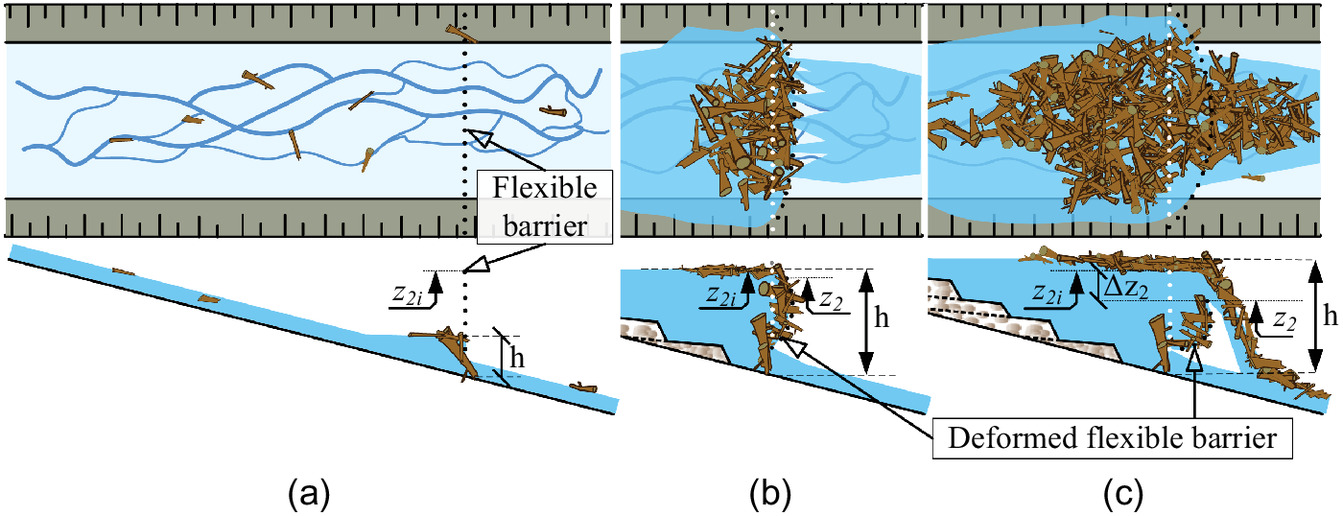
Fig. 1. Sketches of a top view and a side view of the three main phases of a flexible barrier functioning: (a) trapping initiation for high routine events; (b) trapping with increased flow level and associated backwater effect during design events; and (c) release of LW by overtopping during danger events.

Piton et al. (2019, 2020) and Horiguchi et al. (2021), for instance, demonstrated that rigid structures trapping LW might release sudden and massive amounts of LW when overtopped by a sufficiently high depth. It was unclear if such a process might appear on flexible barriers as well. It was questionable that this failure mode observed on rigid barriers would be the same on flexible barriers for two reasons: (1) flexible barriers can obviously deform. The overtopping process is thus possibly more complicated than on rigid barriers because the level of the structure crest, noted as

z_{2}

, tends to decrease under loading [compare Figs. 1(a–c)], thus increasing the overflowing depth

h - z_{2}

that drives the LW overtopping process (Piton et al. 2020). Meanwhile, (2) flexible barriers are extremely porous, which decreases flow levels, increases the flow velocity, stabilizes the LW trapped against the structure (stronger drag forces push the LW against the structure), and LW tends to entangle in the mesh and cables and cannot slide against the structure as against a steel pile or a concrete wall.

To study these processes with small scale modeling, the stiffness and associated deformability of the barrier should therefore be consistent with the prototype scale (Wendeler 2008). This challenge is addressed in the companion paper of Lambert et al. (2022). In essence, the flexible barrier elements (cables and net) were manufactured with a 3D printer using not only a geometry respecting the geometrical similitude, but also material defined to be in mechanical similitude to achieve a relevant barrier deformation. The mechanical behavior of the small scale barrier was validated with elementary tests. Then, using this consistently deformable structure, a comprehensive small scale modeling campaign was conducted to cover the three regimes of functioning (Fig. 1): trapping initiation, full trapping, and end of trapping. This paper presents the results of this campaign. Tests involving mixtures of LW were performed measuring flow depth and trapping efficacy until eventual release occurred by barrier overtopping. Other tests with single logs were performed to study trapping initiation by quantifying their blockage probability for varied flow conditions and bottom clearance.

The paper is organized as follows: a State-of-the-Art section first recalls the main lessons learned from previous works. Material and method are presented second. Third, results are provided regarding the trapping initiation and bottom clearance, the head losses associated with LW, the release conditions, as well as the deformation measured on the barrier when loaded with LW. These results are discussed and exemplified by a case study. The conclusions ultimately close the paper.

State-of-the-Art

For the use of flexible barriers as debris-flow trapping structures, see Wendeler (2008), Volkwein et al. (2011), Volkwein (2014), and Wendeler (2016).

To the best of our knowledge, only Rimböck and Strobl (2002) and Rimböck (2004) studied interactions of flexible barriers with LW [see also recommendations by Lange and Bezzola (2006, pp. 76–81)]. Regarding structural design, Rimböck and Strobl (2002) demonstrated that the dynamic impact of single logs only occurred at the onset of the trapping, when upstream flow velocity remained high along and backwater effects associated with LW trapping were low, thus not slowing down the flows. Consequently, dynamic impact forces were much lower than the pseudo-static force of the barrier obstructed by logs and filled up to the crest. Regarding functional design, Rimböck (2004) provides many relevant recommendations. He recalled that typical mesh apertures, e.g., in the range 0.3–0.5 m, are much smaller than LW, ensuring their trapping. Smaller openings tend to trap small organic matter (leaves and branches) and should thus be avoided. He also stressed that a bottom clearance below the net is necessary to prevent fast clogging even during low flows that would greatly increase maintenance efforts. No clear criterion was however provided, except that the trapping initiation should be sought for flows approaching discharges triggering first damage to elements at risk. Rimböck (2004) also recommends to install flexible barriers in reasonably wide streams (channel width

b_{C} < 15 m

), and relatively straight reaches to prevent uneven LW accumulation and barrier loading (radius of curve

> 10 b_{C}

, barrier located at least

5 b_{C}

downstream of the upstream curves). He also advised not to use flexible barriers in channels with unit discharge

Q / b_{B} > 5 m^{3} / s \cdot m

, with channel unit LW volume

V_{L W} / b_{C} > 20 m^{3} / m

, with channel unit sediment volume

V_{s e d} / b_{C} > 100 m^{3} / m

, with

Q

the water discharge (

m^{3} / s

),

V_{L W}

the solid volume of LW (excluding void) (

m^{3}

),

V_{s e d}

the sediment volume (

m^{3}

),

b_{C}

the channel width (m), and

b_{B}

the barrier width (possibly narrower than the channel) (m). Finally, Rimböck (2004) also advised not to use flexible barriers to trap LW in channels steeper than

\approx 5 %

to ensure that the upstream deposition area has sufficient room to buffer LW and sediment deposition. In steep streams potentially supplying large amounts of sediment, the design of the flexible barrier must absolutely account for both LW, bedload transport, and debris flows. Sediment deposition notably interferes with the trapping of the LW [see additional comments on interactions between sediment deposition and LW accumulation in Rimböck (2004)].

The barrier location should be reasonably easy to access to facilitate surveys and maintenance. It should also not be too far from the protected assets, otherwise LW and sediment might be recruited along the intermediate channel reach. The channel bed should additionally be protected against scouring on the bank on a length of twice the barrier height both upstream and downstream, but also below the barrier to prevent deep scouring and uncontrolled erosion below the structure. This latter recommendation is consistent with the recent works of Schalko et al. (2019b) who observed deep scouring at racks trapping LW: the accumulation of logs tend to float and to redirect flows toward the channel bed, which might result in structure scouring if the bed is mobile.

Rimböck (2004) finally provides an equation to estimate

h

, the flow depth at the barrier. The barrier height

z_{2}

should be higher than

h

z_{2} > h = 4.44 {(\frac{V_{L W}}{b_{C}})}^{c} F M^{0.17} (1 - \frac{35 - K}{105}) \sqrt{\frac{Q}{3 b_{B}}}

(1)

where

F M

is the fine organic matter content,

K

is the Strickler coefficient of the upstream channel bed (

m^{- 1 / 6}

) (see Yen 1992 for the units) and,

c

is a coefficient depending on the channel gradient

S

(

c = 0.20

for

S = 1.0 %

;

c = 0.25

for

S = 3.0 %

, and

c = 0.26

for

S = 5.0 %

).

A careful analysis of Eq. (1) shows that it is not dimensionally homogeneous. The equation is supposed to compute a length (m), while the term on the righthand side has a dimension of (

m^{2 c + 1} s^{- 0.5}

), i.e.

(m^{1.4} s^{- 0.5}) - (m^{1.52} s^{- 0.5})

depending on

c (S)

. The results provided by Eq. (1) are thus scale dependent. Eq. (1) provides good estimates of the measured

h

performed at small scale by Ceron Mayo (2020, p. 27, which were preliminary experiments to this paper). Its application to the same conditions at the prototype scale resulted in overestimations of

h

by a factor of about 2 for the application case performed by Ceron Mayo (2020, p. 39). This bias is on the safe side, because it results in a conservative design of an excessively high barrier, but an update of the approach would be interesting to remove this scale effect. This was one of the objectives of the present paper.

Material and Methods

Flume and Sensors

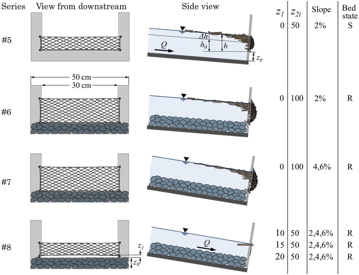
Several series of experiments were performed as described at the end of the “Material and Methods” section. The experimental set up is further described in Ceron Mayo (2020) who performed four preliminary series to the four series presented in this paper. The target scale reduction, for which was defined the barrier similitude regarding both geometrical- and stiffness-scale is

λ = 40

(Lambert et al. 2022). The experiments were conducted in a 6-m long, tilting flume with glass walls having a width

b_{C} = 0.4 m

(i.e., 16 m at prototype scale). Three flume slopes were used:

S = 2 %

, 4%, and 6%. The flume bottom was smooth during experimental series #1–#5 and covered with gravel of diameter 15–20 mm during experimental series #6–#8 (corresponding to a grain diameter of 600 to 800 mm at prototype scale, i.e., a stream bed heavily paved). At the flume outlet, a 10-mm thick transparent plexiglass plate supported the flexible barriers. It was open over a width

b_{B} = 0.3 m

. Flow discharge was varied in the full range of the pump capacity, namely

0.5 - 8 L / s

. It was measured by an electromagnetic flow meter. This range corresponds to

5 - 80 m^{3} / s

at prototype scale, i.e., low to quite high discharges. It expends slightly the range of use suggested by Rimböck (2004) until

Q / b_{B} \approx 6.7 m^{3} / s \cdot m

. The water was injected at the head of the flume through an orifice having the same width as the flume. No sediment feeding device was installed, the experiments thus figure a stream with floods involving mostly water and LW and with marginal sediment transport, consistent with the heavy armoring state of the bed. An ultrasonic probe measured water depth

h

above the bottom of the barrier section. It was located 0.2 m upstream of the barrier, i.e., as close as possible but sufficiently far to avoid noise and influence in the measurement related to the barrier height. Logs sometime were located below the sensor. They never protrude far above the water surface, but it decreases the measurement accuracy which is assumed to be

\pm 2 mm

. Three cable extension transducers were installed horizontally along the top, middle, and bottom of the flexible barriers to measure the barrier elongation. All sensor measurements were recorded on a computer at a 10 Hz frequency. A camera took pictures of the barrier and upstream flume from the ceiling of the laboratory every 10 s. LW mixtures used were weighted before to be supplied in the flume. Logs passing above the barrier were weighted too.

Barrier Tested

The nets had a width of 320 mm (i.e., 12.8 m, respectively at prototype scale). Their height was 50 mm or 100 mm depending of the experimental series (i.e., 2 or 4 m at prototype scale). Two vertical and two horizontal cables, fixed on the Plexiglas support, were used to support the net. The net and cable were manufactured with a 3D printer. Their mechanical strength was defined in similitude with a prototype scale structure (see companion paper by Lambert et al. 2022). The flexible barriers could thus deform in accordance with their loading and their top level tended to decrease realistically.

Large Wood Mixtures and Experimental Protocols

Trapping Initiation: Single Logs Used to Assess the Blockage Probability

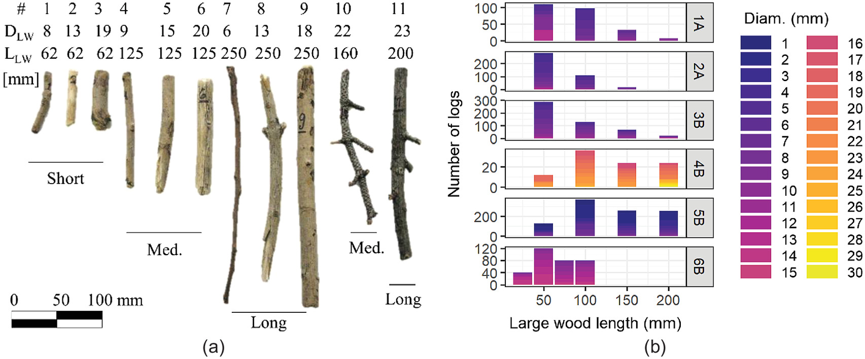
To model trapping initiation, tests were performed with single logs and varying flow discharge, flume slope, and barrier bottom clearance: 10 mm, 15 mm, and 20 mm (i.e., 0.4 m, 0.6 m, and 0.8 m at prototype scale). Eleven different logs were used with varying length, diameter, and presence or absence of branches [Fig. 2(a)]. At prototype scale, these logs have diameter

D_{L W} = 0.24 - 0.76 m

(0.88 m and 0.92 m for the logs with the branches) and length

L_{L W} = 2.5 - 10 m

.

Fig. 2. (a) Pictures of the 11 logs used to assess the trapping initiation; and (b) number of logs of varied length and diameter comprised in each LW mixture used to study head losses and release conditions.

In line with the comprehensive analysis of Furlan et al. (2019, 2020, 2021) who studied the initiation of log trapping at reservoir dam spillways, we aimed at estimating the probability of each log to be trapped when transported alone. Following the recommendation from Furlan et al. (2020), each log was introduced

n_{s u p p l i e d} = 30

times in the flume for each discharge, slope, and bottom clearance. The number of times it was trapped

n_{s t o p p e d}

was recorded and the blockage probability was estimated by

P_{b l o c k a g e} = \frac{n_{s t o p p e d}}{n_{s u p p l i e d}}

(2)

The density of the logs used was not measured but they came from the same Sorbus aucuparia than the one used by Piton et al. (2020) who measured an average LW density of

ρ_{L W} = 0.77

(range of variation: 0.745–0.83). However, contrarily to Furlan et al. (2021), the effect on the blocking probability of the natural field variability of wood density was not studied. We believe that the process of trapping is primarily controlled by the log length, diameter, shape, and the flow discharge, channel slope and barrier bottom clearance, all parameters being studied here; but it is true that further investigation could verify possible effects of other factors as, e.g., wood density, barrier location (e.g. downstream of curves) or channel grain size and morphology.

Filling and Releases: Mixtures of Large Wood

Six LW mixtures were prepared to assess the filling and possible releases [Fig. 2(b) and Table 1]. Mixtures varied in terms of mean log lenght (

L_{L W}

) and maximum log length (

L_{m a x}

), mean log diameter (

D_{L W}

) and maximum log diameter (

D_{m a x}

), total solid LW volume (

V_{L W}

), i.e., excluding void and presence or absence of fine material (

F M

: pine needle figuring small branches). The LW accumulation volume, as well as its content in organic fine material, play a key role in the specific energy head required for the flow to seep through the accumulation, as demonstrated by Schalko et al. (2018, 2019a). Indeed, according to Schalko et al. (2018, 2019a), as the LW accumulation volume and its content in organic fine material increase, the flow is diverted more often through the accumulation body due to the porosity decrease and a more complex flow path, leading to an increase in energy head losses and thus resulting backwater rise

Δ h = h - h_{0}

with

h_{0}

the flow level without LW. According to Schalko et al. (2018), the organic fine material (FM) ranges from 0.03 to 0.15 (for leaves and small wood with a trunk

diameter \leq 0.01 m

) of the LW weight. To account for two extreme cases, within the present work, a slightly higher content of 0.20 was used (in the three mixtures labeled “B”) or no

F M

at all (in the three mixtures labeled “A”). At prototype scale, the LW mixtures have

L_{L W} = 2.6 - 5.2 m

,

L_{m a x} = 4 - 8 m

,

D_{L W} = 0.15 - 0.8 m

,

D_{m a x} = 0.4 - 1.2 m

, and

V_{L W} = 60 - 281 m^{3}

. Such values are representative of high but not extreme LW supply in small mountain streams (e.g., Horiguchi et al. 2015; Ravazzolo et al. 2017; Steeb et al. 2017; Rickli et al. 2018; Ruiz-Villanueva et al. 2019).

Table 1. Main features of the LW mixtures

Code	Units	1A	2A	3B	4B	5A	6B
FM	Yes/No	No	No	Yes	Yes	No	Yes
$L_{L W}$	mm	87	67	82	131	131	66
$D_{L W}$	mm	7.8	6.2	7.4	20.7	3.7	11.8
$L_{m a x}$	mm	200	150	200	200	200	100
$D_{m a x}$	mm	13	13	13	30	10	15
$V_{L W}$	$10^{- 3} m^{3}$	1.036	0.936	2.037	4.39	1.947	2.291

Each run started with a discharge of

1 l / s

and ended until reaching the maximum pump discharge

\approx 8 l / s

or overtopping of the LW, whichever occurred first. The water discharge was increased step by step, by step of usually

1 l / s

. Once the flow level was stable, i.e. approximately 1–3 min after the transitional period related to the change from one discharge stage to another, flow levels were computed as the average value over the next 1–3 min of stable level. Then, discharge was increased to the next step. The level of the upper cable of the barrier was measured with a point gauge but only for series #5 where releases of LW were observed above the barrier. For each slope and flume condition, a first run was performed without wood to know the pure water stage-discharge relationship, and thus later define the LW-related effect on water depth.

LW transport is extremely random in the field (Ruiz-Villanueva et al. 2016; Comiti et al. 2016). Several supply methods were used to address a large range of cases, from sudden massive supply of LW transported almost in an hyper-congested regime (sensu. Ruiz-Villanueva et al. 2019), until logs transported nearly individually. Supply noted “1:1” consisted in feeding the whole mixture in the flume at the first discharge step. One third of the mixture was injected at the three first discharge steps for supply noted “1:3”. Similarly one sixth or one seventh of the mixture was supplied during the first six or seven steps for supplies noted “1:6” or “1:7”, respectively. Since steps were

1 l / s

and the maximum discharge was about

8 l / s

, the latter supply regimes are equivalent to a progressive supply of LW along all the flow rising. We did not address the recession limb of hydrographs in this study.

To also account for the randomness in the accumulation and arrangement of logs, three repetitions were performed for any given couple of mixture and supply mode that was tested. Each run is thus labeled by its mixture code, supply mode, and repetition index (a, b, and c), e.g., “3B(1:7)b” refers to the run with mixture 3B, supply mode 1:7, and second repetition.

Series of Experiments

The experiments presented in this paper were performed after preliminary tests performed by the second author during her Master Thesis and labeled series #1–#4 (Ceron Mayo 2020). Based on these first sequences of four tests series, slight adjustments were brought to the experimental set up before the second sequence. Experiment series #5–#8 were also performed by the second author (see Fig. 3): (1) for series #5, a low net height (

z_{2} = 50 mm

) was used to observe overtopping and releases in the range of discharge that could be tested, and (2) the flume bottom was filled with sediment to figure a natural channel bed rather than the initial smooth bed for series #6–#8. The data gathered during series #1–#4 are available in the appendix of (Ceron Mayo 2020) but are not used in the present study. Table 2 synthesizes the scientific questions studied in each series and eventually mentions the associated adaptation made to the experimental set up. The effect of varying the mixture of LW was mostly studied in series #5 and #6, as well as the effect of the supply mode in the first, thus the higher numbers of measurements in these two series. In series #7, the slope was increased. Overall, 741 data points of discharge, flow depth, and eventual associated LW overtopping weight, were measured during series #5–#7. Blockage probability was assessed during series #8 for 498 different conditions corresponding to

\approx 15,000

observations of a single log being trapped or passing the barrier.

Fig. 3. Sketch of the experimental series and main varying parameters (Bed State: S = smooth; and R = rough). Series #1–#4 were preliminary tests available in Ceron Mayo (2020).

Table 2. Main features of the experimental series

No.	$z_{2}$	N	Object	Adaptation, objective, and main results
5	50	288	HL & R	Widening of the net after the preliminary results of series #1–#4, use of a lower net with height $z_{2} = 50 mm$ to promote overtopping. Many releases.
6	100	286	HL & R	Adding of a rough bed, repetition of tests similar to series #1 with high net to measure backwater rise. No overtopping occurred.
7	100	167	HL & R	High net and test of effect of steeper slope $S = 4 %$ and 6%. No overtopping occurred.
8	50	498	Init.	Set bottom clearances. Tests of trapping initiation with single logs.

Note: $z_{2}$ = flexible barrier height; Object: HL & R = head loss and release test; Init. = analysis of the trapping initiation; and N = number of measurement.

Results

Initiation of the Trapping: The Bottom Clearance

Although these tests were performed within the last experimental series (#8), it seems more logical to present them first as a way to study the beginning of the trapping process. The study of the bottom clearance intended to study the blockage probability

P_{b l o c k a g e}

of single logs. Although

P_{b l o c k a g e}

varies in the range 0 to 1, similar to the trapping efficacy ratio computed as the ratio of trapped volume to the supplied volume (D’Agostino et al. 2000; Shibuya et al. 2010; Horiguchi et al. 2015), both ratios cannot directly be compared. The latter is based on the behavior of groups of logs and encapsulates the progressive capture of key pieces and the subsequent increase of the LW stopping. Conversely, blockage probability

P_{b l o c k a g e}

focuses only on single logs and intends to highlight how the blockade exactly starts, whatever happens later. As such, while high trapping efficacy must be sought (close to one ultimately), it seems sufficient in many cases to seek lower

P_{b l o c k a g e}

. For instance, if

P_{b l o c k a g e} \approx 1 / 3

, it means that, on average, trapping will start as soon as three logs pass. If the trapped piece is a large one, it will then likely partially obstruct the structure and trapping efficacy will increase a great deal for the next supplied LW.

During the 498 measurements of

P_{b l o c k a g e}

, logs were not transported on the rough bed for discharges lower than

Q = 2 - 3 l/ s

. Also,

P_{b l o c k a g e}

was systematically null for flow depths lower than the bottom cable (

h < z_{1}

). Increases in

P_{b l o c k a g e}

appeared with increased log length, log diameter, presence of branches, water discharge, and decreasing bottom clearance.

In order to propose a dimensionless criterion for the bottom clearance

z_{1}

, the ratio of submerged net height (

h - z_{1}

) to log diameter (

D_{L W}

) was first tested (

D_{L W}

accounts for the branches, e.g., logs #10 & #11)

z_{1}^{*} = \frac{h - z_{1}}{D_{L W}}

(3)

Fig. 4(a) shows that

P_{b l o c k a g e}

increases with

z_{1}^{*}

and log length. This increase however appears to be slope-dependent since high blockage probability (e.g.,

P_{b l o c k a g e} ⪆ 0.75

) seems to appear, for instance for long logs [Fig. 4(a), top row], for

z_{1}^{*} \approx 1

at

S = 2 %

, for

z_{1}^{*} \approx 0.3

at

S = 4 %

, and for

z_{1}^{*} \approx 0

at

S = 6 %

. Replacing the measured flow depth (which is not always easy to estimate) by the critical flow depth

h_{c} = {(Q / \sqrt{g b_{B}^{2}})}^{2 / 3}

enables one to get rid of most of the slope dependency [Fig. 4(b)]

z_{1}^{*} = \frac{h_{c} - z_{1}}{D_{L W}} = \frac{{(\frac{Q}{\sqrt{g b_{B}^{2}}})}^{2 / 3} - z_{1}}{D_{L W}}

(4)

Fig. 4. Blockage probability against (a) $z_{1}^{*} = [(h - z_{1}) / (D_{L W})]$ ; and (b) $z_{1}^{*} = [(h_{c} - z_{1}) / (D_{L W})]$ , for varied slopes (columns) and log length (rows). Continuous lines show mean trends. Evidence of increasing of $P_{b l o c k a g e}$ with $z_{1}^{*}$ but also with the slope and log length, as well as with the ratio of log diameter to bottom clearance $D_{L W} / z_{1}$ represented by the dot size.

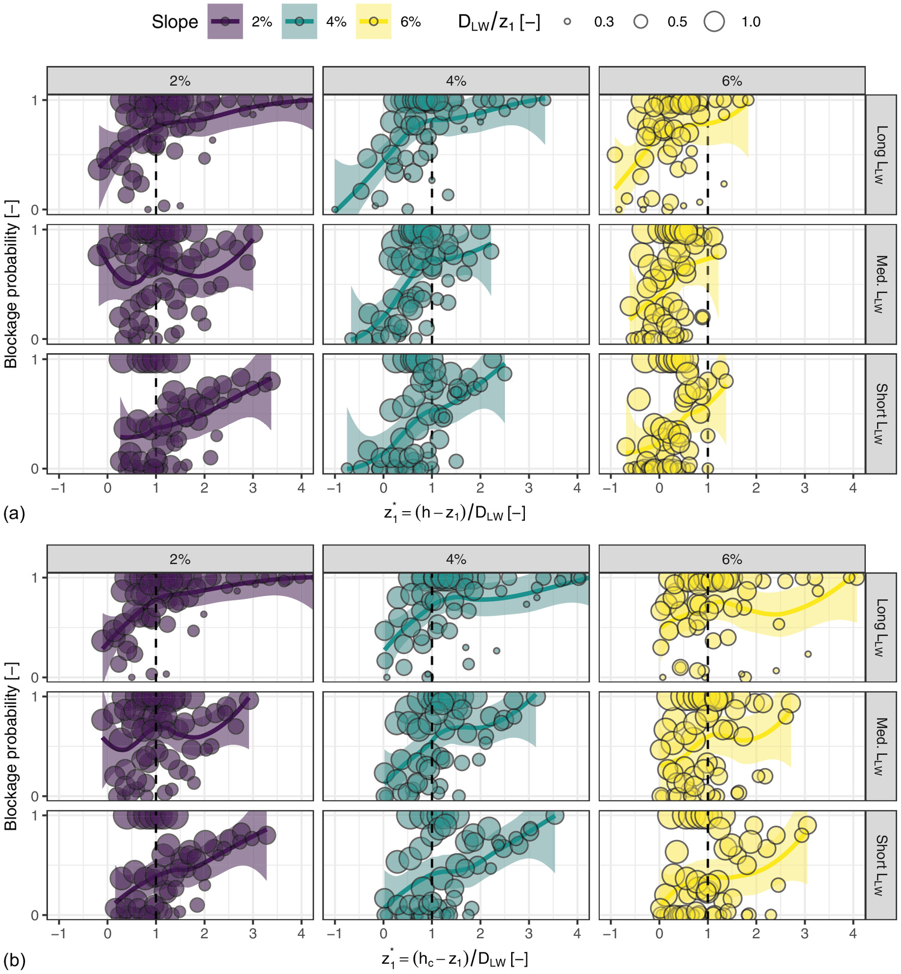
It is worth stressing that in using Eq. (4),

z_{1}^{*}

is no longer an actual submerged depth but rather aggregates the three main parameters driving the blockage: the barrier bottom clearance, the log diameter, and the flow unit discharge.

All data, irrespective of the slope, are gathered in Fig. 5 using Eq. (4) to compute

z_{1}^{*}

. Each row refers to a range of log length. Fig. 5(a) demonstrates the overlapping of the mean trends for the three slopes tested. The criterion is thus nearly slope-independent in the 2%–6% range. Fig. 5(b) shows that not only the dimensionless submerged depth

z_{1}^{*}

matters, but also the ratio of the log diameter to the bottom clearance

D_{L W} / z_{1}

. Mean trends are plotted as lines in both Figs. 5(b and c) for two sub-samples. For thick logs (

D_{L W} / z_{1} > 1

),

P_{b l o c k a g e}

is

\approx 50 %

when

z_{1}^{*}

is close to 0 and exceeds 75% for

z_{1}^{*} > 1

, being even equal to one for long logs. Meanwhile, for thinner logs (

D_{L W} / z_{1} < 1

),

P_{b l o c k a g e} \approx 50 %

, 25%, and 5% for

z_{1}^{*} = 1

and long, medium, and short logs, respectively.

P_{b l o c k a g e}

becomes very high (

> 75 %

) only for

z_{1}^{*} > 3

for these logs of smaller diameter. This demonstrates that thick and/or long logs are intuitively much easier to trap, but also that logs might pass a flexible barrier even if the latter is submerged on more than the log diameter. Drag forces simply suck the log below the structure that may in addition deform upward.

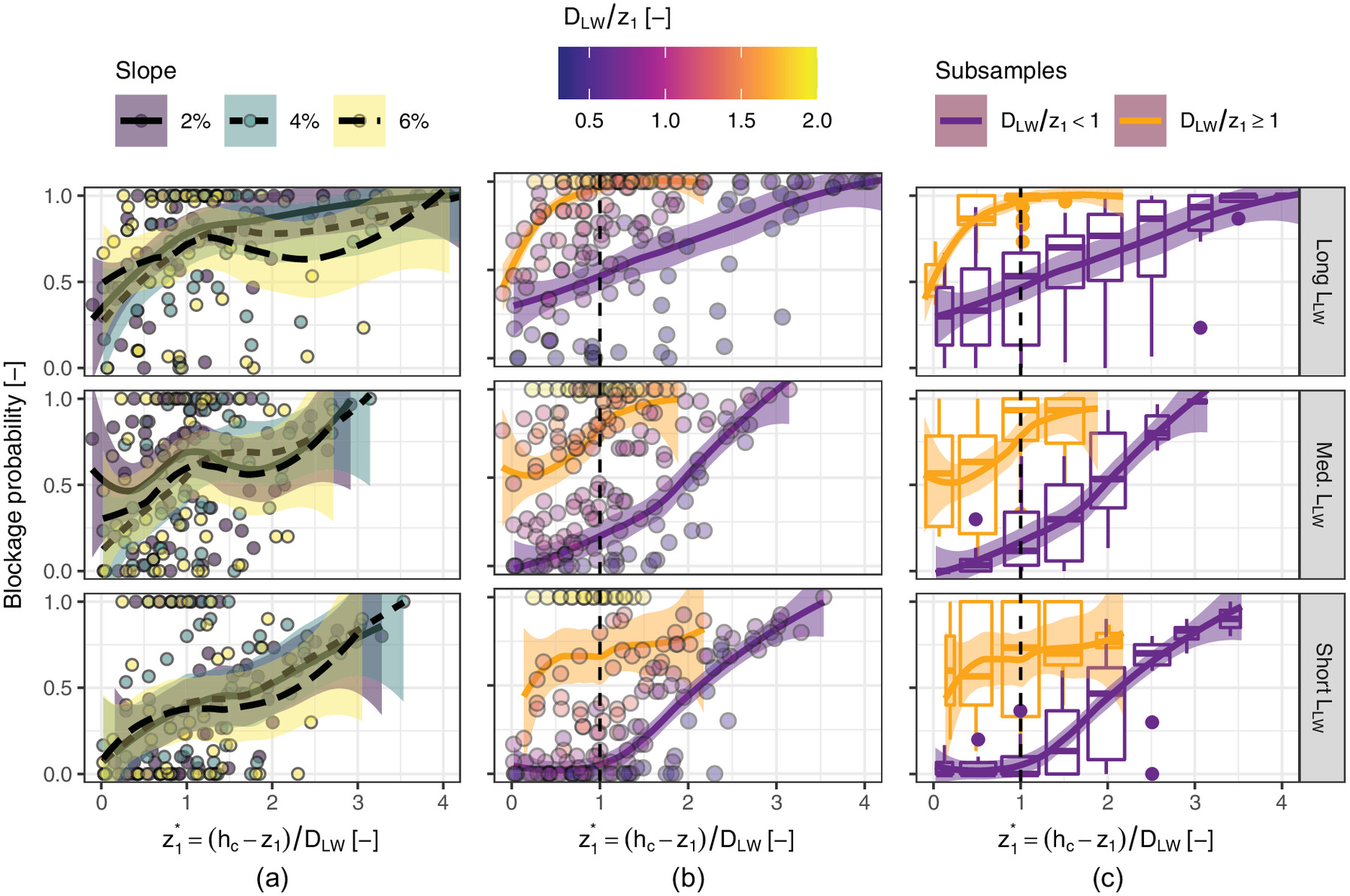
Fig. 5. Synthesis of blockage probability $P_{b l o c k a g e}$ of *single logs*: (a) overlapping mean trends (lines and associated ribbons) for varied slope, evidence of the disappearance of the slope dependency; (b) evidence of increasing $P_{b l o c k a g e}$ with $D_{L W} / z_{1}$ ; and (c) mean trends for the two sub-samples of thick logs and fine logs.

The diameter of LW pieces varies according to the type and age of riparian forests. We recommend using the criteria of Fig. 5 in an inverse approach: for a given target water discharge at which LW trapping would be necessary (or not), the user will find how much is the

P_{b l o c k a g e}

for small and high values of

D_{L W}

based on the mean trends of Fig. 5(c). A few iterations varying

z_{1}

enables to define an appropriate bottom clearance preventing excessively high trapping probability that would trigger high maintenance costs, while having a non-null trapping probability for flows for which trapping is necessary.

As a design criteria, we suggest to select

z_{1}

considering the discharge of floods potentially carrying a significant amount of LW. The bottom clearance can be selected such that

z_{1}^{*} \approx 1

on rivers where the passage of some medium and short logs, as well as a handful of long one, is acceptable. This can be relaxed to

z_{1}^{*} \approx 0

if the site can accommodate some long elements. Conversely, on extremely sensitive sites,

z_{1}^{*} \approx 3

is rather recommended, but such a drastic value may lead to very small bottom clearance and much heavier maintenance effort. See also the Case study section at the end of the paper for a complementary use of this criteria.

Main Phases of Trapping

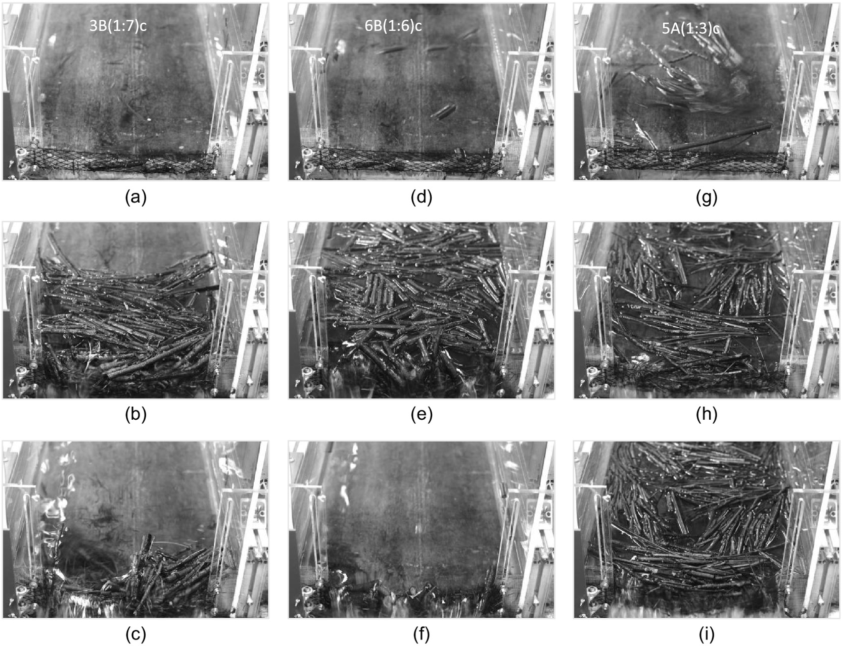
The following sections are based on experiments aiming to study the trapping and eventual release processes. Three main phases of accumulation were eventually observed [yet described in Lange and Bezzola (2006) and Wendeler (2008, p. 54)]: (1) trapping initiation with a few logs hitting the barrier and adopting a transverse position [Figs. 6(a, d, and g)]. A few elements might protrude under or through the net. As soon as a few logs are trapped, the subsequent single logs reaching the barrier are almost certainly trapped. (2) Accumulation phase where blockage probability is one. Logs accumulate against the barrier and progressively load it. As soon as a few logs are trapped, they obstruct the flow section and trigger a backwater effect. Flow velocities decrease drastically upstream and logs form a “floating carpet” [Figs. 6(b, e, h, and i)]. For high slope and discharge, a few elements may be sucked below the free surface and rather build a multi-layered, denser LW accumulation. (3) A release phase was observed on only a few cases [e.g., Figs. 6(c and f)]. We define a “release” by the sudden and uncontrolled transfer of many logs downstream of the barrier [criterion:

cumulated mass > 10 %

of the whole mixture for a single flow discharge, as in Piton et al. (2020)]. Flow conditions enabling releases were systematically related to high overflowing (

h > z_{2}

), similar to dam spillways (Furlan et al. 2021; Bénet et al. 2021; Vaughn et al. 2021) or open check dams (Piton et al. 2020). Consequently, all overtopping were observed on the small net (series #5) and none on the 100-mm high nets.

Fig. 6. Phases of trapping of a low flexible barrier ( $z_{2} = 50 mm$ , Series #5). Run 3B(1:7)b (i.e., mixture 3B, supply mode 1:7, second repetition): (a) initiation; (b) filled structure and a few seconds later; and (c) state after release; Run 6B(1:6)c: (d) initiation; (e) filled structure and a few seconds later; and (f) state after release; and Run 5A(1:3)b: (g) initiation; (h) half-filled structure; and (i) filled structure (no release despite significant overflowing).

Backwater Rise Related to Large Wood

The equivalent upstream Froude number

F r_{0}

was computed with the channel width

b_{C}

and water depth without LW

h_{0}

, and assuming a uniform flow, it would be equivalent to the depth out of the backwater area.

F r_{0} = Q / \sqrt{g b_{C}^{2} h_{0}^{3}}

varies in the range

0.5 - 0.65

for

S = 2 %

,

F r_{0} \approx 1.1

for

S = 4 %

and

F r_{0} \approx 1.4

for

S = 6 %

. Upstream flow conditions are thus typical of steep, coarse gravel-bed channels. Since the flume bottom is fixed at the barrier by the Plexiglas sheet, it cannot be scoured (see sketches on Fig. 3). Our configuration is thus similar to a flexible barrier installed on a bed sill. The flexible barrier being located at the flume outlet, it was not influenced by the downstream flow level, a reasonable hypothesis regarding the relatively high

F r_{0}

and the weir presence. It can be seen that when looking at cross-shaped dots on Figs. 7 and 8, the flow depth at the barrier, without LW, can be approximated by a weir equation (i.e.,

Q \propto b_{B} H_{0}^{1.5}

), providing that one uses the specific energy head

H

rather than the depth

h

in the equation, e.g., in a rectangular channel

H_{0} = h_{0} + \frac{Q^{2}}{2 g b_{C}^{2} h_{0}^{2}} = h_{0} (1 + F r_{0}^{2} / 2)

Q = μ b_{B} \sqrt{2 g H_{0}^{3}} \approx μ b_{B} \sqrt{2 g h_{0}^{3} {(1 + \frac{F r_{0}^{2}}{2})}^{3}}

(5)

with

μ

as the weir coefficient, calibrated at 0.45 in our case (see the agreement between black lines and cross-shaped dots in Figs. 7 and 8). Note that the upstream specific energy head is computed using the channel flow velocity, i.e., over the whole channel width

b_{C}

, rather than with the weir width

b_{B}

. Accounting for the inertia term

Q^{2} / (2 g b_{C}^{2} h_{0}^{2})

is necessary when the approximation

h \approx H

falls in defect, e.g., if

F r > 0.3

in a rectangular channel and accepting a 5% error on

H

:

H = h + [Q^{2} / (2 g h^{2} b_{C}^{2})] = h {1 + [Q^{2} / (2 g h^{3} b_{C}^{2})]} = h [1 + (F r^{2} / 2)] > 1.05 h

. Note that the effect of the flexible barrier can be neglected when no clog it, because it is extremely porous (void ratio

\approx 80 %

). When logs begin to be trapped, they obstruct the channel section and increase the upstream flow depth. A gradually varied free surface profile then emerges: an M1-profile for the subcritical flows observed with

S = 2 %

and an S1-profile for the supercritical flows observed with

S = 4 %

and

S = 6 %

(sensu Te Chow 1959, p. 226), the transition between the supercritical and the subcritical flows occurring within a undular jump.

Fig. 7. Flow depth $h$ against water discharge $Q$ . Dot color refers to the LW mixture used (Fig. 2). Dot size is correlated with the relative mass of LW released during the measurement step. The black lines are computed using Eq. (5). The light gray lines show the level of the top cable as it varies if it was measured: (a) Series #5 with a small net, smooth bed; (b) Series #6 (high net, rough bed); and (c) Series #7 (high net, rough bed, steeper slope).

Fig. 8. (a) Relative energy head loss $β = (Δ H / H_{0})$ against water discharge $Q$ . Colored lines shows mean trends for each slope. Side boxplots are computed on the sub-sample related to each slope tested. Evidence of an enveloppe value of 1.75. (b) Flow depth $h$ against water discharge $Q$ : measurements and predictions of Eq. (7) with varying reduction rate coefficient.

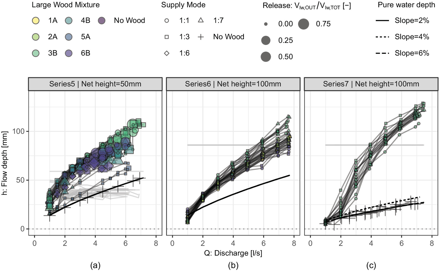
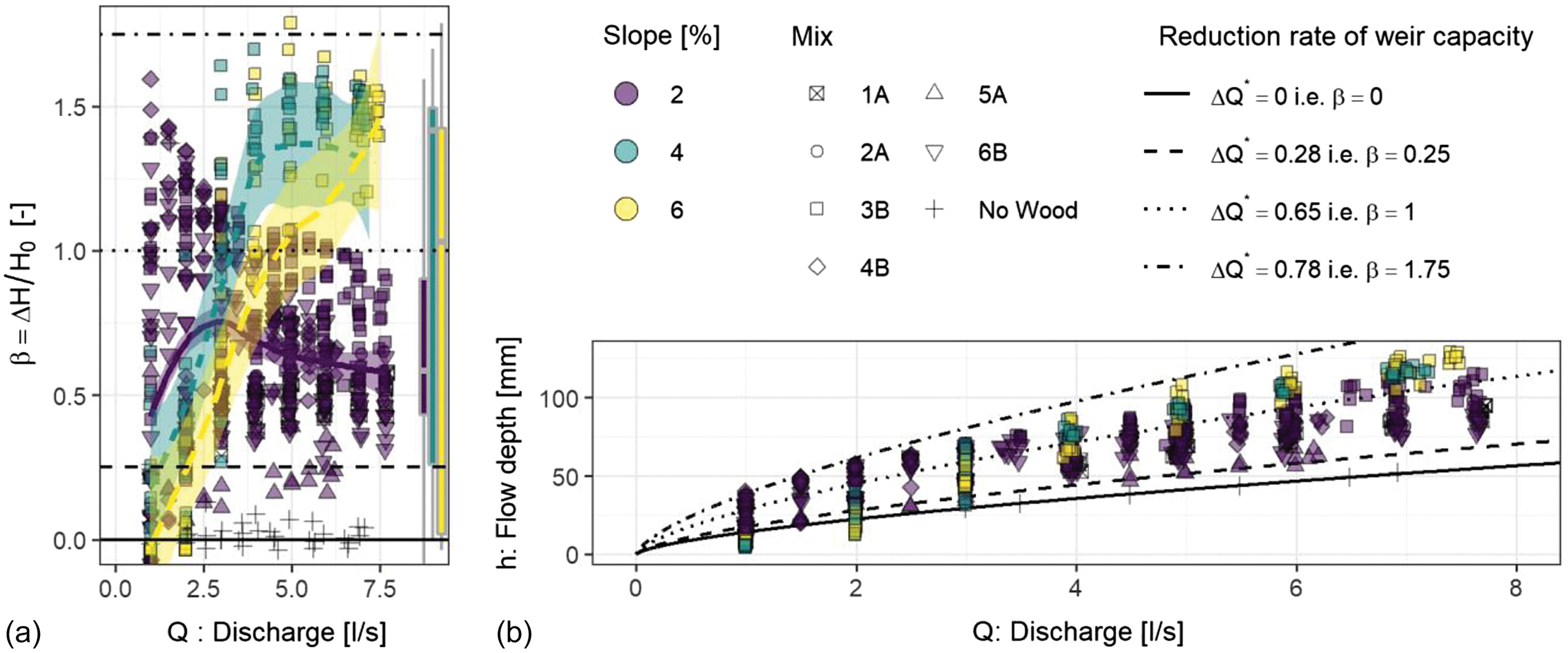
Fig. 7 shows flow depth

h

against water discharge

Q

with and without LW. Increase of

h

with

Q

is obvious, as well as the LW-related backwater rise represented by the deviation of the measurement dots to the black lines representing the pure water depth computed with Eq. (5). The last series of experiments, performed with a rough bed and without artificial obstruction, are more plausible to compare with field sites [Figs. 7(b and c)]. Series #5 was performed to focus on the release phase. Its smooth bed is less directly comparable with field sites [Fig. 7(a)]. Depths measured during series #7 are higher because of the increased flow specific energy on the steeper slopes (

S = 4 %

and 6%), as compared to the condition of series #6 performed with

S = 2 %

[compare Figs. 7(b and c)].

In this paper, the effect of LW on water depth, i.e., the rise of the free surface level necessary for the flow to gain sufficient energy to seep through the LW accumulation, thus losing this energy gain, is called “LW-related backwater rise” or “LW-related head loss”. Since the approaching flow conditions have relatively high Froude numbers and thus non-negligible inertial terms, the LW-related head losses are analyzed with the energy head loss

Δ H = H - H_{0}

, rather than just using the depths

h

and

h_{0}

and the associated backwater rise

Δ h = h - h_{0}

used in other works (e.g., Schmocker and Hager 2013; Schalko et al. 2018). Meanwhile, flow conditions at the barrier are systematically subcritical with

F r < 0.3

once clogged and the specific energy head could be approximated by the depth

H \approx h

(it means that

Q^{2} / 2 g b_{C}^{2} h^{2} ≪ h

, the left term being small not because the discharge

Q

is small but because the water depth is high). Data analysis showed that the LW-related relative energy head losses

Δ H / H_{0}

varied in the range 0–1.75 [Fig. 8(a)]. Many small values of

Δ H / H_{0}

are observed for low discharge, i.e., for flow conditions where either, not the whole LW volume, was supplied (supply modes 1:3, 1:6 and 1:7), or some supplied pieces did not reach the barrier and were still stuck on the rough bed (for

Q < 3 l / s

). Relative energy head loss thus tends to increase with

Q

during the first phase of barrier clogging but then decreases. The actual depth

h

increases continuously (Fig. 7), these decreases observed for the three slope trends are thus related to a relatively higher increase of the approaching specific energy head

H_{0}

as compared to the increase of

h

at the barrier. The difference in trends between measurements on

S = 2 %

and the similar patterns of

S = 4 %

and 6% is likely due to denser LW accumulations built by the supercritical flows of the steeper slope. On the gentler slope, LW accumulations were subjected to lower velocities and drag forces, and were thus slightly less dense.

When obstructed with LW, the flexible barrier triggers a significant energy head loss. Interestingly, the general behavior was still similar to a weir equation, i.e.,

Q \propto b_{B} h^{1.5}

, though the equivalent weir coefficient was much lower than without LW. Two ways can be used to account for the LW-related energy head loss when computing flow depth

h

at the flexible barrier: (1) by assuming a relative energy head loss

β = (Δ H / H_{0})

[Eq. (6)] as proposed in (Piton et al. 2020), or (2) by assuming a reduction ratio of the discharge

Δ Q^{*}

[Eq. (7)] in the line of the approach proposed by Bénet et al. (2021, 2022) for reservoir dam spillways

Q = μ b_{B} \sqrt{2 g {(\frac{h}{1 + β})}^{3}}

(6)

Q = (1 - Δ Q^{*}) μ b_{B} \sqrt{2 g h^{3}}

(7)

The first formulation enables to directly reads the relative increase in water depth as compared with flow without wood, e.g., if

β = 0.2

, it means that flow level increases by 20% in presence of LW. The second formulation gives a sense of the flow capacity reduction at known flow depth. Table 3 provides a selection of values of both parameters computed using

Δ Q^{*} = 1 - {[1 + (Δ H / H_{0})]}^{- 3 / 2}

. Fig. 8(b) shows both the measured depths and the prediction of Eq. (7) for varying discharge. It shows that using

Δ Q^{*} = 0.78

(computed with

β = (Δ H / H_{0}) = 1.75

) provides an envelope curve of all our measurements. In essence, a heavily clogged flexible barrier has a similar behavior than a weir discharging only

22 % = 1 - Δ Q^{*} = 1 - 0.78

of its full capacity. A barrier having an average clogging state might convey twice this discharge (

Δ Q^{*} \approx 0.65

) depending on random processes related both to supply, i.e., low or high recruitment and transfer of LW to the barrier, supply of fine material or only of large pieces; and accumulation too, e.g., variably dense, evenly distributed (or not). When using Eq. (7) with

Δ Q^{*} = 0.65

, i.e., the mean value on our sample, the ratio between the observed depth and the predicted depth varied in the range 0.2–1.7, half of the values being in the range 0.9–1.3.

Table 3. Relative energy head loss and associated discharge reduction coefficient

$β = \frac{Δ H}{H_{0}}$	$Δ Q^{*}$	Value used for	Source
0	0	Pure water conditions	—
0.25	0.28	Lower envelope of flexible barrier	This paper
0.5	0.46	Upper range on dam spillways	Hartlieb (2017)
0.6	0.51	Upper range for slit and slot dams	Piton et al. (2020)
1.0	0.65	Average behavior of flexible barrier	This paper
1.1	0.67	Upper range for racks	Piton et al. (2020)
1.5	0.75	Upper range for racks	Schalko et al. (2019a)
1.75	0.78	Upper envelope curve of flexible barrier	This paper

It could be possible to propose more sophisticated equations including the volume of LW, its fine matter content, and the size of the logs, e.g., mean or maximum length or diameters, as proposed by others (Schalko et al. 2018, 2019a). Such parameters, accurately known in small scale experiments, are however unknown and strongly variable in the field:

V_{L W}

for instance varies over two orders of magnitude for catchments of similar sizes or other features (e.g., FOEN 2019, pp. 27–28). We thus chose to provide a simple approach to compute an average case (

Δ Q^{*} = 0.65

, computed with

(Δ H / H_{0}) = 1.0

), a high obstruction case (

Δ Q^{*} = 0.78

), and a low obstruction case (

Δ Q^{*} = 0.28

) as shown in Fig. 8(a) and Table 3. We trust the users to define the “what if” scenarios they want to address and to chose the associated dimensionless numbers.

Release Condition of Large Wood Overtopping

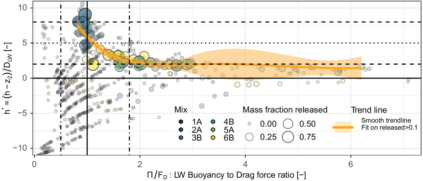
Similar to previous works, release conditions were first analyzed in the light of the dimensionless overflowing depth

h^{*}

h^{*} = \frac{h - z_{2}}{D_{L W}}

(8)

The release of LW over dam spillways occurs for

h^{*} > 1.5 - 2

(Pfister et al. 2013; Furlan et al. 2021; Bénet et al. 2021; Vaughn et al. 2021). Upstream of such structures, LW accumulates as extended floating carpets made of a single layer of LW. Conversely, LW tends to get stuck at open check dams as denser, multi-layered accumulations thanks to the higher approaching velocities allowed by the higher structure porosity. Piton et al. (2020) and Horiguchi et al. (2021) demonstrated that these thicker accumulations are more stable than on closed structures and their releases occur for

h^{*} > 3 - 8

(also because some logs get entangled in the openings and form sort of random anchors, increasing the structure’s retention capacity).

Flexible barriers are even more porous than open check dams. Consistently, natural releases of LW were difficult to obtain during the experiments. The size of dots on Fig. 7 varies with the volume of LW released. Significant releases, i.e.,

> 10 %

of the mixture volume, only occurred during series #5 (net height of 50 mm). The releases occurred in a range of

h^{*} > 3 - 8

, similar to open check dams. It is worth noting that specifically low flexible barriers were manufactured to observe the LW release: the 50-mm high barrier would be a small scale model of a 2-m high barrier at scale 1:40.

To get a more precise picture of the effect of the approaching flow conditions building dense accumulation or, on the contrary, lousy floating carpet, the dimensionless ratio of buoyancy to drag force introduced by Piton et al. (2020) on rigid barriers was also computed

Π / F_{D} \approx \frac{π}{2 C_{D}} \frac{ρ - ρ_{L W}}{ρ} \frac{g D_{L W} b_{C}^{2} h^{2}}{Q^{2}}

(9)

with the buoyancy force

Π = (π / 4) g (ρ - ρ_{L W}) D_{L W}^{2} L_{L W}

, the drag force

F_{D} = (1 / 2) ρ C_{D} D_{L W} L_{L W} v_{f}^{2}

, the fluid density

ρ

, the log density

ρ_{L W}

, the fluid velocity

v_{f}

, and the log drag coeffient

C_{D}

taken as 1.2 (following Merten et al. 2010). These formulations rely on the following hypotheses (Piton et al. 2020) : (1) logs have a transverse position as compared to flow direction, (2) they are nearly fully submerged, thus their whole volume is considered in

Π

and their whole projected area in

F_{D}

, (3) LW are stopped by the barrier and experience the drag force of the full flow velocity, (4) the mean section velocity is a good approximation of the fluid velocity near the log

v_{f} \approx \frac{Q}{b_{C} \cdot h}

, and (5) the channel is rectangular (otherwise, the mean flow velocity estimation and the Froude number equation must be adjusted). Considering these hypotheses,

Π / F_{D}

, as many other dimensionless numbers, is not meant to give an accurate estimation of whether or not a given log will sink. It only gives a general sense of the balance between drag force and buoyancy. It has notably the following limits: it ignores inter-logs effects, antecedent flows, or 3D flow patterns (Piton et al. 2020).

Fig. 9 shows

h^{*}

versus

Π / F_{D}

with the size of dots increasing with the amount of LW released. The study of release conditions requires to understand the distribution of large dots. It appears clearly that in slow flow conditions, i.e.,

Π / F_{D} ≫ 1

, depths leading to overtopping are similar to the known value for dam spillways (

h^{*} \approx 2

). On average, depths triggering releases progressively increase to

h^{*} \approx 5

and even higher when flow conditions become prone to creating dense, multi-layered accumulation, namely when drag force gets close to buoyancy (

Π / F_{D} \approx 1

), though random variations appear. For fast flow conditions (

Π / F_{D} < 1

), LW piles up. Large parts of these thick accumulations might be released for randomly varying overflowing depths in the range

h^{*} \approx 4 - 8

.

Fig. 9. Flow conditions considering relative overflowing depth $h^{*} = [(h - z_{2}) / D_{L W}]$ and buoyancy to drag force ratio $Π / F_{D}$ with dot size proportional to the amount of LW released. Vertical lines shows the transition zone near $Π / F_{D} = 1$ (continuous line = exact value, dashed-dotted line = range of uncertainty accounting for a 20% relative uncertainty on the density and $C_{D} = 0.9 - 1.41$ according to Ruiz-Villanueva et al. 2020). Evidence of increased mean and variability of $h^{*}$ with decreasing $Π / F_{D}$ , i.e., faster flows.

While the method proposed to compute flow depth [Eq. (7)] did not account for parameters related to LW, release conditions are strongly controlled by their diameter (mean diameter in the mixture

D_{L W}

) which appear in both dimensionless numbers,

Π / F_{D}

and

h^{*}

.

In steep slope streams, LW is mostly composed of single logs without branches or rootwads (Rickli et al. 2018). However, the presence of a few of them would likely increase the stability of the LW accumulation and increase values of

h^{*}

leading to releases as observed by Pfister et al. (2013) on PK-weirs. The threshold values of

h^{*}

we highlight in this work are thus conservative regarding this effect.

Loading Measurement

The elongation along the horizontal direction of the flexible barrier was measured at three locations: (1) along the upper cable, (2) at the middle of the net where no supporting cable was installed to maximize deformation, and (3) along the bottom cable (Fig. 10). With the net structure being more flexible than the supporting cable, the deformation at the middle was larger. An additional test (repeated twice) was performed with a plastic sheet obstructing the net to compare the loading and associated deformation related to LW with full hydrostatic loading [Fig. 10(e)]. The plastic sheet was pleated to make sure that it did not hold part of the pressure. The blue lines in Figs. 10(a–c) show the associated deformation. Fig. 10(d) shows the ratio between the measured deformation with LW and mean value of deformation for full hydrostatic loading at the same flow level. For low flow level

h / z_{2} < 0.7

only, both the net and the bottom cable experience higher deformation with LW than full hydrostatic load. It might be an artifact of the measurement accuracy (the deformations are on average less than 1% in this range). It could also be that part of the drag force applied by the flow on the logs is transferred on the net through force chains between logs. Conversely, it is clear that when flow levels reach the barrier crest (

h \geq z_{2}

), the deformations measured with LW are systematically lower than with full hydrostatic loading (ratio of elongation with LW/hydrostatic elongation, mean±standard deviation:

0.59 \pm 0.12

,

0.32 \pm 0.04

,

0.21 \pm 0.07

for the lower cable, middle of the net, and upper cable, respectively). The potential drag force transfer from logs to the barrier was likely negligible at this stage because the high backwater rise reduces flow velocity to low values. In addition, LW accumulation was dense and partially held and transferred forces to the rigid side wings of the barrier, so equivalent effects would appear on rough banks (Rimböck 2004).

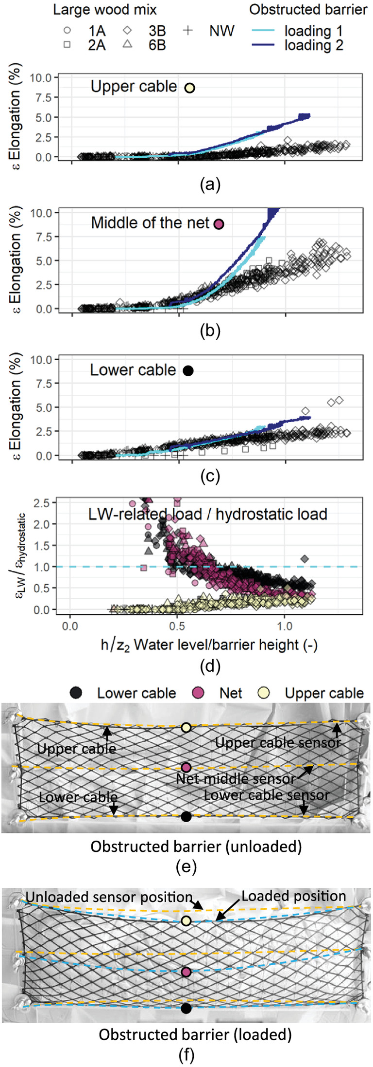
Fig. 10. Elongation of the barrier depending of the water level: the dots are values measured with LW while the blue lines are tests performed with a barrier obstructed by a flexible plastic sheet applying a full hydrostatic load on the barrier: (a) upper cable; (b) middle of the net; (c) bottom cable; (d) ratio of deformation with LW $ε_{L W}$ divided by the deformation due to full hydrostatic loading $ε_{h y d r o s t a t i c}$ ; (e) picture of the obstructed barrier before loading; and (f) loaded obstructed barrier.

In case more fine material than in our experiences are supplied, it might build denser and less porous and permeable LW accumulations that would eventually transfer a higher loading than in our measurement. We however demonstrated that the accumulated drag forces and the flow pressure on the logs located against the barrier remained lower than a full hydrostatic load. For the structural design of a flexible barrier intending to trap LW (and not sediment), as yet suggested by Rimböck (2004), it seems that a reasonable first order assumption is to apply a full hydrostatic loading.

Discussion

Insights, Limitations, and Remaining Open Questions

This work pushed further the pioneering work of Rimböck and Strobl (2002) and Rimböck (2004) by using a flexible barrier capable of deforming in a realistic way, and by addressing both the initiation of the trapping and its limits leading to releases by overtopping. It shows that a very dense accumulation of LW can form at flexible barriers based on their high permeability allowing flow to seep through and stick the logs on the entire flow section. The associated increases in flow depth were high, higher than what was typically observed on the rigid barrier as reported in Table 3 (see also Piton et al. 2020, for a more comprehensive analysis of data reported in the literature).

Although this work explores the aforesaid scientific gaps, it has obvious limitations. As in any hydraulic small scale model, it was impossible to meet full dynamic similitude (Heller 2011). The Reynolds number similitude was relaxed because the flows were fully turbulent (

R e = Q / b_{B} / ν > 2,600

for all measurements, with

ν

as water kinematic viscosity). The surface tension

σ

might have an effect on measurements at shallow depths, 95% of measurements had Weber number

W e = ρ g h^{2} / σ > 24

(the threshold value is given between 10 and 120 according to Peakall and Warburton 1996). Consequently, data with flow depth

h

lower than a certain threshold should be considered with caution. Peakall and Warburton (1996), Erpicum et al. (2016), and Fritz and Hager (1998) suggest minimum depths of 1.5 cm, 3.0 cm, and 4.0 cm in different types of studies, respectively, i.e., 6%, 13%, and 22% of our measurements might be doubtful, respectively. They were mostly the values measured without LW. Thus, we are more confident in our data with high discharge and water depth, i.e., the most interesting data anyway.

In addition, it is worth stressing that sediment transport was ignored in this experimental work, which is an extremely important limitation. On steeper slopes, and more generally if significant bedload transport is involved, the whole question of interaction between water, LW, sediment, and flexible barriers becomes certainly much more complicated. This would deserve new experiments and further research (see the State-of-the-Art section for the available guidelines).

Although we believe that the manufactured flexible barrier used in this work is a step forward in hydraulic small scale modeling, it is true that real wood pieces were used to model logs. Their stiffness is thus not down-scaled. As compared to reality, they are abnormally stiff, as well as resistant to breakage. We believe that the high stiffness of our logs is not a big issue. Relaxing this similitude would be a problem if, in the field, LW trapped against flexible barriers were strongly deformed and bent by flows. We demonstrated that the structure, and thus the logs stuck against it, are subjected to an effort of more or less a hydrostatic loading and that flow velocities near the barrier are very low. Tree trunks and large branches are not significantly deformed by such a loading. For instance, standing trees in the floodplain regularly trap LW and act as a barrier (e.g., Abbe and Montgomery 2003). If a hydrostatic loading would bend and break them, we hypothesize that this trapping process would not be observed as often in the field. Meanwhile, in rapidly flowing river reaches, when trees are scoured and recruited by flows, they get broken when falling or when blocked against obstacles and being impacted by fast flows, other LW, and boulders (FOEN 2019, pp. 52–54). This second effect was accounted for by using logs with reduced lengths as compared with actual tree heights.

Applicability to Gentler Slopes

This experimental campaign was performed with relatively steep slopes (2%, 4%, and 6%) and Froude numbers ranging from 0.5 to 1.4 for flow without barrier. Use of the results on cases with significantly different conditions should be careful. For cases of gentler slope, flow velocities are usually lower, and thus drag forces too, and

Π / F_{D}

is higher. Thus, flows progressively lose their ability to pile-up logs and to suck them below water and the barrier. We suspect that for flow conditions where only floating carpets can form (

F r ≪ 1

and

Π / F_{D} ≫ 1

), the trapping initiation would then be better captured by Eq. (3) rather than Eq. (4). Regarding LW-related head losses, it can be anticipated that in such flow conditions, logs would more likely stay at the surface and would less likely obstruct the bottom of the structure, thus with reduced head losses. Hartlieb (2012, 2017), for instance, studied LW-related head losses on dam spillways strongly overflowing before the logs were supplied. Accumulations were sometime multi-layered but did not obstruct the whole structure height. In approaching Froude numbers ranging from 0.05–0.35, the associated relative head losses varied in the range

Δ h / h_{0} = 0.05 - 0.5

, i.e., much less than in our experiments. Regarding release conditions, the

h^{*}

versus

Π / F_{D}

criteria already accounts for possible low velocities, and was shown to be consistent with other references coming from dam spillway experiments, i.e., with quieter flows.

Case Study Example: The Torrent Des Glaciers

An example of application of the criteria developed in the present paper is proposed here below on the Torrent des Glaciers. At this location, the catchment area is

114 {km}^{2}

. Peak discharges with return periods of 10 years, 100 years, and 1,000 years are

Q_{10} = 47 m^{3} / s

,

Q_{100} = 102 m^{3} / s

, and

Q_{1000} = 203 m^{3} / s

, respectively (Arnaud et al. 2014). The mean diameter of the LW supplied by the catchment is assumed to be 0.25 m. The flexible barrier is intended to be fully functional for

Q_{100}

, potential trapping needing maintenance operation is acceptable for

Q > Q_{10}

. The structure would be installed in gorges with strong bedrock sidewalls. In these gorges, the channel is heavily armored with large boulders and sediment transport is assumed marginal. The channel width is 15 m and the slope 5%.

In pure water conditions, the flow depth is approximated by a critical flow depth (continuous line in Fig. 11). The bottom cable is initially suggested to be set at the flow depth for

Q_{10}

:

z_{1} = 1 m \approx h (Q_{10})

. Eq. (4) is used to define the discharge for which trapping might start (

z_{1}^{*} = 0

), becomes probable (

z_{1}^{*} = 1

), and finally is certain (

z_{1}^{*} = 3

). As can be seen in Fig. 11, trapping is probable for a discharge in between

Q_{10}

and

Q_{100}

and is certain near

Q_{100}

. Considering that these criteria describe the trapping of single, isolated logs and that, once a few logs are trapped, the trapping efficacy becomes almost total, this analysis validate the choice of setting the bottom cable at

Q_{10}

.

Fig. 11. Synthetic stage—discharge curve exemplifying the design of a flexible barrier for large wood trapping on the Torrent des Glaciers (FR). Eq. (7) is used with various values of $Δ Q^{*}$ to compute flow—stage-discharge curves. Trapping initiation is computed with Eq. (4) and selected values of $z_{1}^{*}$ . Release conditions are computed with Eq. (8) and values of h* selected after computation of $Π / F_{D}$ using Eq. (9).

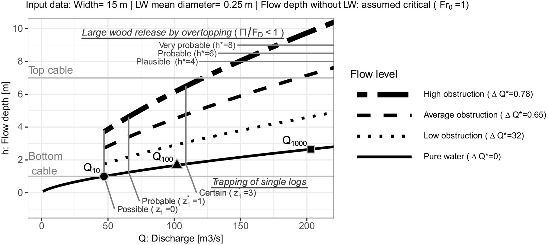
Flow depth in the presence of trapped LW is computed using Eq. (7) and various hypotheses of

Δ Q^{*}

. The hypothesis of high obstruction (

Δ Q^{*} = 0.78

) leads to a flow depth of 6.2 m for

Q_{100}

. Using a net height of 6 m enables us to set the top cable at

z_{2} = (z_{1} + 6) = 7 m

, i.e., reasonably above the maximum depth for the project design flood of

Q_{100}

. For the whole range of discharge possibly involving LW trapping (

Q > Q_{10}

) and every hypotheses of obstructions, applying Eq. (9) shows that

Π / F_{D} < 1

, i.e., that the LW accumulation is likely dense and piling up. A reasonable result regarding the steepness of the site.

Neglecting the top cable lowering (this should be refined in a further step when structural design is defined), it is possible to compute the flow depth at which LW release become plausible (

h^{*} = 4

), probable (

h^{*} = 6

) and very probable (

h^{*} = 8

) using Eq. (8). These values are selected in the light of the

Π / F_{D}

range. One can see on Fig. 11 that such flow depths are reached in between 150 and

175 m^{3} / s

, i.e., well above

Q_{100}

in the worst case of high obstruction, and are not reached for

Q < Q_{1000}

in cases of average or low obstruction. This functional failure probability is also considered satisfying and validates the net height.

Conclusions

When hydraulic structures like bridges and dams cannot be adapted to let LW pass through, it is sometimes necessary to trap LW upstream to prevent their eventual obstruction. Depending on the site peculiarities, filtrating structures as open check dams, racks, or flexible barriers are usually relevant options.

This paper presents a comprehensive analysis of the interactions of LW with flexible barriers. It intends to complement the pioneer and isolated so far works of Rimböck and Strobl (2002) and Rimböck (2004). It is based on small scale model experiments. Four scientific questions were addressed:

•

The initiation of the trapping of logs was studied with eleven logs having variable shapes and sizes. Their blockage probability was studied for a range of flow conditions and bottom clearance below the barrier. A new dimensionless number was introduced to predict the increasing likelihood of a single log being trapped with increasing unit discharge and log diameter and length and decreasing bottom clearance.

•

Tests with six mixtures of LW were then performed to study the LW-related head losses. It was shown that accumulations of LW against flexible barriers increased flow levels, sometimes up to 2.75 times the specific energy head computed without LW. The flow depth at the barrier can be computed using a weir equation with an extra coefficient of flow reduction rate (reduction of 65% on average, upper bound: 78%).

•

When subjected to high overflowing, flexible barriers might suddenly release a large share of the LW trapped. Such releases can be very dangerous and should be anticipated. Overall, they occurred for depths over the crest in the range of 2–8 times the LW mean diameter. Computing the dimensionless ratio of buoyancy to drag forces with Eq. (9) helps to refine this range by defining whether this phenomenon is likely to occur for relatively low overflowing depths (in case flow conditions are slow enough to let LW accumulate as a lousy floating carpet), or if drag forces are high enough to pile-up logs which build accumulations more stable and having a more random behavior.

•

Sensors measured the barrier deformation when loaded by LW-laden flows, but also during tests with full hydrostatic loading. It proved that when the flow level is close or higher than the barrier crest, deformations with LW were lower than the full hydrostatic loading. The latter can be used as a first, conservative assumption for the structural design of flexible barriers trapping LW.

These experiments were performed using small scale flexible barriers that deformed quite consistently with reality. A companion paper explains how to tackle the issue of manufacturing a small scale flexible barrier which has a target stiffness better capturing the actual deformability of these structures (Lambert et al. 2022). It was done by introducing a new similitude criterion on the stiffness modulus of the barrier materials. The cables and net forming the flexible barrier were then manufactured with a 3D printer and targeted material characteristics.

A case study finally exemplified an application of the design criteria proposed in this paper. This work was performed following a first similar analysis on rigid barriers (weirs, slit dams, slot dams and racks, see Piton et al. 2020). The fact that the crest level of flexible barriers progressively decreases with the filling and loading of the structure was expected to be potentially dangerous because it would increase the overflowing depth, and thus promote eventual releases of LW. Meanwhile, the extremely high permeability of flexible barriers enables very high discharges and thus limits flow levels, when compared to a rigid body structure with less permeability. Finally, flexible barriers proved to be very efficient and relevant structures to trap LW because the advantage of their high porosity has a stronger effect on flow levels and release conditions when compared with the small drawback that the barrier crest level decreased when loaded.

Notation

The following symbols are used in this paper:

$b_{B}$: width of the flow at the barrier (m);
$b_{C}$: width of the channel upstream of the barrier (m);
$C_{D}$: log drag coefficient;
$D_{L W}$: arithmetic mean log diameter (m);
$D_{m a x}$: diameter of the thickest logs (m);
$F_{D}$: drag force (N);
$F M$: ratio of volume of fine material (thin branches, leaves) over LW volume;
$F r$: Froude number just upstream of the barrier: $F r \approx (Q / \sqrt{g b_{C}^{2} h^{3}})$ ;
$F r_{0}$: Froude number of the approaching flow without LW $F r_{0} \approx (Q / \sqrt{g b_{C}^{2} h_{0}^{3}})$ ;
$g$: acceleration due to gravity ( $9.81 m / s^{2}$ );
$H$: specific energy head at the barrier $H = h + [(Q^{2}) / (2 g b_{C}^{2} h^{2})]$ (m);
$H_{0}$: specific energy head without large wood $H_{0} = h_{0} + [(Q^{2}) / (2 g b_{C}^{2} h_{0}^{2})]$ (m);
$h$: flow depth above the bottom level of the barrier section (m);
$h^{*}$: dimensionless overflowing water depth $h^{*} = [(h - z_{2}) / (D_{L W})]$ ;
$h_{0}$: flow depth at the barrier without LW (m);
$K$: Strickler coefficient of the channel ( $m^{- 1 / 6}$ );
$L_{L W}$: arithmetic mean log length (m);
$L_{m a x}$: length of the longest logs (m);
$n_{s t o p p e d}$: number of test where the introduced log was trapped by the barrier (logs);
$n_{s u p p l i e d}$: number of test where the log was introduced in the flume (logs);
$P_{b l o c k a g e}$: blockage probability of a single log;
$Q$: water discharge ( $m^{3} / s$ );
Re: Reynolds number $R e = Q / b_{B} / ν$ ;
$S$: slope of the flume ( $m / m$ );
$V_{L W}$: solid volume of the mixture, i.e., without void ( $m^{3}$ );
$V_{s e d}$: volume of sediment supplied by the design event ( $m^{3}$ );
$v_{f}$: relative velocity of the flow near the logs ( $m / s$ );
$W e$: weber number $W e = ρ g h^{2} / σ$ ;
$z_{0}$: weir height below the flexible barrier (m);
$z_{1}$: level of the bottom cable on the net (m);
$z_{2}$: level of the top cable on the net (m);
$β$: relative energy head loss $Δ H / H_{0}$ ;
$Δ H$: energy head loss = $H - H_{0}$ (m);
$Δ h$: backwater rise = $h - h_{0}$ (m);
$Δ Q^{*}$: dimensionless discharge capacity loss related to LW;
$μ$: weir coefficient, 0.45 in our case;
$ν$: water kinematic viscosity taken as $10^{- 6}$ ( $m^{2} / s$ );
$Π$: buoyancy force (N);
$ρ$: density of the fluid;
$ρ_{L W}$: LW density;
$σ$: air-water surface tension, taken as 0.072 (N/m);
$ε_{h y d r o s t a t i c}$: horizontal deformation of the flexible by a full hydrostatic load ( $m / m$ ); and
$ε_{L W}$: horizontal deformation of the flexible loaded with LW ( $m / m$ ).

Data Availability Statement

All data generated or used during the study are available in a repository online in accordance with funder data retention policies: FilTor: Interaction between flexible barriers and flows (INRAE), https://data.inrae.fr/dataverse/filtor, Trapping initiation: https://doi.org/10.15454/CHHYIX, backwater rise and LW releases: https://doi.org/10.15454/RMIEJM, and flexible barrier elongation measurement: https://doi.org/10.15454/9HUDGG.

Acknowledgments

The authors would like to thanks Firmin Fontaine, Hervé Bellot, Alexis Buffet, and Christian Eymond-Gris for their assistance and support in the preparation of the flume and measurement devices. This work was funded by the French Ministry of Environment (Direction Générale de la Prévention des Risques—Ministère de la Transition Ecologique et Solidaire) within the multirisk Agreement SRNH-IRSTEA 2019 (Action FILTOR). The authors are grateful to the three anonymous referees who provided many helpful comments on previous versions of this paper.

References

Abbe, T. B., and D. R. Montgomery. 2003. “Patterns and processes of wood debris accumulation in the Queets river basin, Washington.” Geomorphology 51 (1–3): 81–107. https://doi.org/10.1016/S0169-555X(02)00326-4.

Google Scholar

Albaba, A., S. Lambert, F. Kneib, B. Chareyre, and F. Nicot. 2017. “Dem modeling of a flexible barrier impacted by a dry granular flow.” Rock Mech. Rock Eng. 50 (11): 3029–3048. https://doi.org/10.1007/s00603-017-1286-z.

Google Scholar

Arnaud, P., Y. Aubert, D. Organde, P. Cantet, C. Fouchier, and N. Folton. 2014. “Estimation de l’aléa hydrométéorologique par une méthode par simulation: La méthode SHYREG: Présentation—Performances—Bases de données.” Houille Blanche (2): 20–26. https://doi.org/10.1051/lhb/2014012.

Google Scholar

Ashwood, W., and O. Hungr. 2016. “Estimating total resisting force in flexible barrier impacted by a granular avalanche using physical and numerical modeling.” Can. Geotech. J. 53 (10): 1700–1717. https://doi.org/10.1139/cgj-2015-0481.

Google Scholar

Badoux, A., N. Andres, and J. Turowski. 2014. “Damage costs due to bedload transport processes in Switzerland.” Nat. Hazards Earth Syst. Sci. 14 (2): 279–294. https://doi.org/10.5194/nhess-14-279-2014.

Google Scholar

Bénet, L., G. De Cesare, and M. Pfister. 2021. “Reservoir level rise under extreme driftwood blockage at ogee crest.” J. Hydraul. Eng. 147 (1): 04020086. https://doi.org/10.1061/(ASCE)HY.1943-7900.0001818.

Google Scholar

Bénet, L., G. De Cesare, and M. Pfister. 2022. “Partial driftwood rack at gated ogee crest: Trapping rate and discharge efficiency.” J. Hydraul. Eng. 148 (8): 06022008. https://doi.org/10.1061/(ASCE)HY.1943-7900.0001994.

Google Scholar

Braudrick, C. A., G. E. Grant, Y. Ishikawa, and H. Ikeda. 1997. “Dynamics of wood transport in streams: A flume experiment.” Earth Surf. Processes Landforms 22 (7): 669–683. https://doi.org/10.1002/(SICI)1096-9837(199707)22:7%3C669::AID-ESP740%3E3.0.CO;2-L.

Google Scholar

Brighenti, R., A. Segalini, and A. M. Ferrero. 2013. “Debris flow hazard mitigation: A simplified analytical model for the design of flexible barriers.” Comput. Geotech. 54 (Oct): 1–15. https://doi.org/10.1016/j.compgeo.2013.05.010.

Google Scholar

Ceron Mayo, A. R. 2020. “Flexible barriers and trapping of large wood.” M.S. thesis, Ecole Nationale Supérieure de l’Energie, l’Eau et l’Environnement, Univ. Grenoble Alpes.

Google Scholar

Comiti, F., A. Luca, and D. Rickenmann. 2016. “Large wood recruitment and transport during large floods: A review.” Geomorphology 269 (Sep): 23–39. https://doi.org/10.1016/j.geomorph.2016.06.016.

Google Scholar

D’Agostino, V., M. Degetto, and M. Righetti. 2000. “Experimental investigation on open check dam for coarse woody debris control.” In Vol. 20 of Dynamics of water and sediments in mountain basins, Quaderni di Idronomia Montana, 201–212. Cosenza, Italy: Bios.

Google Scholar

De Cicco, P. N., E. Paris, V. Ruiz-Villanueva, L. Solari, and M. Stoffel. 2018. “In-channel wood-related hazards at bridges: A review.” River Res. Appl. 34 (7): 617–628. https://doi.org/10.1002/rra.3300.

Google Scholar

Erpicum, S., B. P. Tullis, M. Lodomez, P. Archambeau, B. J. Dewals, and M. Pirotton. 2016. “Scale effects in physical piano key weirs models.” J. Hydraul. Res. 54 (6): 692–698. https://doi.org/10.1080/00221686.2016.1211562.

Google Scholar

FOEN (Federal Office for the Environment). 2019. Bois flottant dans les cours d’eau. Berne, CH: FOEN.

Google Scholar

Friedrich, H., D. Ravazzolo, V. Ruiz-Villanueva, I. Schalko, G. Spreitzer, J. Tunnicliffe, and V. Weitbrecht. 2022. “Physical modelling of large wood (LW) processes relevant for river management: Perspectives from New Zealand and Switzerland.” Earth Surf. Processes Landforms 47 (1): 32–57. https://doi.org/10.1002/esp.5181.

Google Scholar

Fritz, H. M., and W. H. Hager. 1998. “Hydraulics of Embankment Weirs.” J. Hydraul. Eng. 124 (9): 963–971. https://doi.org/10.1061/(ASCE)0733-9429(1998)124:9(963).

Google Scholar

Furlan, P., M. Pfister, J. Matos, C. Amado, and A. J. Schleiss. 2019. “Experimental repetitions and blockage of large stems at ogee crested spillways with piers.” J. Hydraul. Res. 57 (2): 250–262. https://doi.org/10.1080/00221686.2018.1478897.

Google Scholar

Furlan, P., M. Pfister, J. Matos, C. Amado, and A. J. Schleiss. 2020. “Statistical accuracy for estimations of large wood blockage in a reservoir environment.” Environ. Fluid Mech. 20 (3): 579–592. https://doi.org/10.1007/s10652-019-09708-7.

Google Scholar

Furlan, P., M. Pfister, J. Matos, C. Amado, and A. J. Schleiss. 2021. “Blockage probability modeling of large wood at reservoir spillways with piers.” Water Resour. Res. 57 (8): e2021WR029722. https://doi.org/10.1029/2021WR029722.

Google Scholar

Gschnitzer, T., B. Gems, B. Mazzorana, and M. Aufleger. 2017. “Towards a robust assessment of bridge clogging processes in flood risk management.” Geomorphology 279 (Feb): 128–140. https://doi.org/10.1016/j.geomorph.2016.11.002.

Google Scholar

Hartlieb, A. 2012. “Large scale hydraulic model tests for floating debris jams at spillways.” In Vol. C18 of Proc., 2nd IAHR European Congress, 1–6. München, Germany: International Association for Hydro-Environment Engineering and Research.

Google Scholar

Hartlieb, A. 2017. “Decisive parameters for backwater effects caused by floating debris jams.” Open J. Fluid Dyn. 7 (4): 475–484. https://doi.org/10.4236/ojfd.2017.74032.

Google Scholar

Heller, V. 2011. “Scale effects in physical hydraulic engineering models.” J. Hydraul. Res. 49 (3): 293–306. https://doi.org/10.1080/00221686.2011.578914.

Google Scholar

Horiguchi, T., G. Piton, M. Munir, and V. Mano. 2021. “Driftwood and hybrid debris barrier interactions: Process of trapping and prevention of releases during overtopping of releases during overtopping.” In Proc., 14th INTERPRAEVENT Congress, 206–215. Klagenfurt, Austria: International Research Society Interpraevent.

Google Scholar

Horiguchi, T., H. Shibuya, S. Katsuki, N. Ishikawa, and T. Mizuyama. 2015. “A basic study on protective steel structures against woody debris hazards.” Int. J. Prot. Struct. 6 (2): 191–215. https://doi.org/10.1260/2041-4196.6.2.191.

Google Scholar

Lambert, S., F. Bourrier, A. R. Ceron-Mayer, L. Dugelas, F. Dubois, and G. Piton. 2022. “Small-scale modeling of flexible barriers. I: Mechanical similitude of the structure.” J. Hydraul. Eng. 149 (3): 04022043. https://doi.org/10.1061/JHEND8.HYENG-13070.

Google Scholar

Lange, D., and G. Bezzola. 2006. “Schwemmholz—Probleme und Lösungsansätze.” Accessed December 8, 2022. https://ethz.ch/content/dam/ethz/special-interest/baug/vaw/vaw-dam/documents/das-institut/mitteilungen/2000-2009/188.pdf.

Google Scholar

Leonardi, A., F. K. Wittel, M. Mendoza, R. Vetter, and H. J. Herrmann. 2016. “Particle-fluid-structure interaction for debris flow impact on flexible barriers: Debris flow impact on flexible barriers.” Comput.-Aided Civ. Infrastruct. Eng. 31 (5): 323–333. https://doi.org/10.1111/mice.12165.

Google Scholar

Mazzorana, B., V. Ruiz-Villanueva, L. Marchi, M. Cavalli, B. Gems, T. Gschnitzer, L. Mao, A. Iroumé, and G. Valdebenito. 2018. “Assessing and mitigating large wood-related hazards in mountain streams: Recent approaches.” J. Flood Risk Manage. 11 (2): 207–222. https://doi.org/10.1111/jfr3.12316.

Google Scholar

Merten, E., J. Finlay, L. Johnson, R. Newman, H. Stefan, and B. Vondracek. 2010. “Factors influencing wood mobilization in streams.” Water Resour. Res. 46 (10): W10514. https://doi.org/10.1029/2009WR008772.

Google Scholar

Ng, C. W. W., D. Song, C. E. Choi, R. C. H. Koo, and J. S. H. Kwan. 2016. “A novel flexible barrier for landslide impact in centrifuge.” Géotech. Lett. 6 (3): 221–225. https://doi.org/10.1680/jgele.16.00048.

Google Scholar

Peakall, J., and J. Warburton. 1996. “Surface tension in small hydraulic river models—The significance of the Weber number.” J. Hydrol. 35 (2): 199–212.

Google Scholar

Pfister, M., D. Capobianco, B. Tullis, and A. J. Schleiss. 2013. “Debris-blocking sensitivity of piano key weirs under reservoir-type approach flow.” J. Hydraul. Eng. 139 (11): 1134–1141. https://doi.org/10.1061/(ASCE)HY.1943-7900.0000780.

Google Scholar

Piton, G., T. Horigushi, L. Marchal, and S. Lambert. 2020. “Open check dams and large wood: Head losses and release conditions.” Nat. Hazards Earth Syst. Sci. 20 (12): 3293–3314. https://doi.org/10.5194/nhess-20-3293-2020.

Google Scholar

Piton, G., V. Mano, D. Richard, G. Evin, D. Laigle, J. Tacnet, and P. Rielland. 2019. “Design of a debris retention basin enabling sediment continuity for small events: The Combe de Lancey case study (France).” In Proc., 7th Int. Conf. on Debris-Flow Hazards Mitigation, 1019–1026. Golden, CO: Debris Flow Hazards Mitigation Association.

Google Scholar

Piton, G., and A. Recking. 2016a. “Design of sediment traps with open check dams. I: Hydraulic and deposition processes.” J. Hydraul. Eng. 142 (2): 04015045. https://doi.org/10.1061/(ASCE)HY.1943-7900.0001048.

Google Scholar

Piton, G., and A. Recking. 2016b. “Design of sediment traps with open check dams. II: Woody debris.” J. Hydraul. Eng. 142 (2): 04015046. https://doi.org/10.1061/(ASCE)HY.1943-7900.0001049.

Google Scholar

Ravazzolo, D., L. Mao, B. Mazzorana, and V. Ruiz-Villanueva. 2017. “Brief communication: The curious case of the large wood-laden flow event in the Pocuro stream (Chile).” Nat. Hazards Earth Syst. Sci. 17 (11): 2053–2058. https://doi.org/10.5194/nhess-17-2053-2017.

Google Scholar

Rickenmann, D., A. Badoux, and L. Hunzinger. 2015. “Significance of sediment transport processes during piedmont floods: The 2005 flood events in Switzerland.” Earth Surf. Processes Landforms 41 (2): 224–230. https://doi.org/10.1002/esp.3835.

Google Scholar

Rickli, C., A. Badoux, D. Rickenmann, N. Steeb, and P. Waldner. 2018. “Large wood potential, piece characteristics, and flood effects in Swiss mountain streams.” Phys. Geogr. 39 (6): 542–564. https://doi.org/10.1080/02723646.2018.1456310.

Google Scholar

Rimböck, A. 2004. “Design of rope net barriers for woody debris entrapment. Introduction of a design concept.” In Proc., Int. Congress Interpraevent, 265–276. Klagenfurt, Austria: International Research Society Interpraevent.

Google Scholar

Rimböck, A., and T. Strobl. 2002. “Loads on rope net constructions for woody debris entrapment in torrents.” In Proc., Int. Congress Interpraevent, 797–807. Klagenfurt, Austria: International Research Society Interpraevent.

Google Scholar

Royet, P., G. Degoutte, L. Peyras, J. Lavabre, and F. Lemperrière. 2010. “Cotes et crues de protection, de sûreté et de danger de rupture.” Houille Blanche (2): 51–57. https://doi.org/10.1051/lhb/2010018.

Google Scholar

Ruiz-Villanueva, V., et al. 2019. “Characterization of wood-laden flows in rivers.” Earth Surf. Processes Landforms 44 (9): 1694–1709. https://doi.org/10.1002/esp.4603.

Google Scholar

Ruiz-Villanueva, V., A. Díez-Herrero, J. A. Ballesteros, and J. M. Bodoque. 2014. “Potential large woody debris recruitment due to landslides, bank erosion and floods in mountain basins: A quantitative estimation approach.” River Res. Appl. 30 (1): 81–97. https://doi.org/10.1002/rra.2614.

Google Scholar

Ruiz-Villanueva, V., C. Gamberini, E. Bladé, M. Stoffel, and W. Bertoldi. 2020. “Numerical modeling of instream wood transport, deposition, and accumulation in braided morphologies under unsteady conditions: Sensitivity and high-resolution quantitative model validation.” Water Resour. Res. 56 (7): e2019WR026221. https://doi.org/10.1029/2019WR026221.

Google Scholar

Ruiz-Villanueva, V., H. Piégay, A. M. Gurnell, R. A. Marston, and M. Stoffel. 2016. “Recent advances quantifying the large wood dynamics in river basins: New methods and remaining challenges: Large Wood Dynamics.” Rev. Geophys. 54 (3): 611–652. https://doi.org/10.1002/2015RG000514.

Google Scholar

Schalko, I. 2020. “Wood retention at inclined racks: Effects on flow and local bedload processes.” Earth Surf. Processes Landforms 45 (9): 2036–2047. https://doi.org/10.1002/esp.4864.

Google Scholar

Schalko, I., C. Lageder, L. Schmocker, V. Weitbrecht, and R. Boes. 2019a. “Laboratory flume experiments on the formation of spanwise large wood accumulations part I: Effect on backwater rise.” Water Resour. Res. 55 (6): 4854–4870. https://doi.org/10.1029/2018WR024649.

Google Scholar

Schalko, I., C. Lageder, L. Schmocker, V. Weitbrecht, and R. Boes. 2019b. “Laboratory flume experiments on the formation of spanwise large wood accumulations part II: Effect on local scour.” Water Resour. Res. 55 (6): 4871–4885. https://doi.org/10.1029/2019WR024789.

Google Scholar

Schalko, I., L. Schmocker, V. Weitbrecht, and R.-M. Boes. 2018. “Backwater rise due to large wood accumulations.” J. Hydraul. Eng. 144 (9): 04018056. https://doi.org/10.1061/(ASCE)HY.1943-7900.0001501.

Google Scholar

Schmocker, L., and W. Hager. 2011. “Probability of drift blockage at bridge decks.” J. Hydraul. Eng. 137 (4): 470–479. https://doi.org/10.1061/(ASCE)HY.1943-7900.0000319.

Google Scholar

Schmocker, L., and W. H. Hager. 2013. “Scale modeling of wooden debris accumulation at a debris rack.” J. Hydraul. Eng. 139 (8): 827–836. https://doi.org/10.1061/(ASCE)HY.1943-7900.0000714.

Google Scholar

Shibuya, H., S. Katsuki, H. Ohsumi, N. Ishikawa, and T. Mizuyama. 2010. “Experimental study on woody debris trap performance of drift wood capturing structure.” J. Jpn. Soc. Erosion Control Eng. 63 (3): 34–41. https://doi.org/10.11475/sabo.63.3_34.

Google Scholar

Steeb, N., D. Rickenmann, A. Badoux, C. Rickli, and P. Waldner. 2017. “Large wood recruitment processes and transported volumes in Swiss mountain streams during the extreme flood of August 2005.” Geomorphology 279 (Feb): 112–127. https://doi.org/10.1016/j.geomorph.2016.10.011.

Google Scholar

Te Chow, V. 1959. Vol. 1 of Open-channel hydraulics. New York: McGraw-Hill.

Google Scholar

Vaughn, T., B. M. Crookston, and M. Pfister. 2021. “Floating woody debris: Blocking sensitivity of labyrinth weirs in channel and reservoir applications.” J. Hydraul. Eng. 147 (11): 06021016. https://doi.org/10.1061/(ASCE)HY.1943-7900.0001937.

Google Scholar

Volkwein, A. 2014. Flexible debris flow barriers: Design and application. Birmensdorf, Switzerland: WSL Berichte, Swiss Federal Institute for Forest, Snow and Landscape Research.

Google Scholar

Volkwein, A., C. Wendeler, and G. Guasti. 2011. “Design of flexible debris flow barriers.” Ital. J. Eng. Geol. Environ. 1093–1100. https://doi.org/10.4408/IJEGE.2011-03.B-118.

Google Scholar

Wendeler, C. 2016. Debris-flow protection systems for mountain torrents. Basic principles for planning and calculation of flexible barriers. Birmensdorf, Switzerland: Swiss Federal Institute for Forest, Snow and Landscape Research WSL.

Google Scholar

Wendeler, C., A. Volkwein, B. W. McArdell, and P. Bartelt. 2018. “Load model for designing flexible steel barriers for debris flow mitigation.” Can. Geotech. J. 56 (6): 893–910. https://doi.org/10.1139/cgj-2016-0157.

Google Scholar

Wendeler, C. S. I. 2008. “Murgangrückhalt in Wildbächen: Grundlagen zu Planung und Berechnung von flexiblen Barrieren.” Ph.D. thesis, Dept. of Civil, Environment and Geomatics, ETH Zurich.

Google Scholar

Wohl, E., et al. 2019. “The natural wood regime in rivers.” Bioscience 69 (4): 259–273. https://doi.org/10.1093/biosci/biz013.

Google Scholar

Yen, B. C. 1992. “Dimensionally homogeneous manning’s formula.” J. Hydraul. Eng. 118 (9): 1326–1332. https://doi.org/10.1061/(ASCE)0733-9429(1992)118:9(1326).

Google Scholar

Information & Authors

Information

Published In

Journal of Hydraulic Engineering

Volume 149 • Issue 3 • March 2023

Copyright

This work is made available under the terms of the Creative Commons Attribution 4.0 International license, https://creativecommons.org/licenses/by/4.0/.

History

Received: Sep 14, 2021

Accepted: Oct 21, 2022

Published online: Dec 27, 2022

Published in print: Mar 1, 2023

Discussion open until: May 27, 2023

Authors

Affiliations

Guillaume Piton, Ph.D. https://orcid.org/0000-0002-0124-0909 [email protected]

Researcher, Univ. Grenoble Alpes, INRAE, CNRS, IRD, Grenoble INP, IGE, Grenoble 38000, France (corresponding author). ORCID: https://orcid.org/0000-0002-0124-0909. Email: [email protected]

View all articles by this author

Ana Rocio Ceron-Mayo

Master’s Student, Univ. Grenoble Alpes, INRAE, CNRS, IRD, Grenoble INP, IGE, Grenoble 38000, France.

View all articles by this author

Stéphane Lambert, Ph.D. https://orcid.org/0000-0003-2221-0589 [email protected]

Researcher, Univ. Grenoble Alpes, INRAE, CNRS, IRD, Grenoble INP, IGE, Grenoble 38000, France. ORCID: https://orcid.org/0000-0003-2221-0589. Email: [email protected]

View all articles by this author

Metrics & Citations

Metrics

Citations

Download citation

If you have the appropriate software installed, you can download article citation data to the citation manager of your choice. Simply select your manager software from the list below and click Download.

Cited by

Deep Roy, Michele Palermo, Simone Pagliara, Control of Surface Plastic Transport in Natural Streams, Journal of Hydraulic Engineering, 10.1061/JHEND8.HYENG-13832, 150, 4, (2024).
Abstract
Stéphane Lambert, Franck Bourrier, Ana Rocio Ceron-Mayo, Loïc Dugelas, Fabien Dubois, Guillaume Piton, Small-Scale Modeling of Flexible Barriers. I: Mechanical Similitude of the Structure, Journal of Hydraulic Engineering, 10.1061/JHEND8.HYENG-13070, 149, 3, (2022).
Abstract

Abstract

Introduction

State-of-the-Art

Material and Methods

Flume and Sensors

Barrier Tested

Large Wood Mixtures and Experimental Protocols

Trapping Initiation: Single Logs Used to Assess the Blockage Probability

Filling and Releases: Mixtures of Large Wood

Series of Experiments

Results

Initiation of the Trapping: The Bottom Clearance

Main Phases of Trapping

Backwater Rise Related to Large Wood

Release Condition of Large Wood Overtopping

Loading Measurement

Discussion

Insights, Limitations, and Remaining Open Questions

Applicability to Gentler Slopes

Case Study Example: The Torrent Des Glaciers

Conclusions

Notation

Data Availability Statement

Acknowledgments

References

Information

Published In

Copyright

History

Authors

Affiliations

Metrics

Citations

Download citation

Cited by

Figures

Other

Share

Copy the content Link

Share with email

Share

Request Username

Create a new account

Change Password

Password Changed Successfully

Verify Phone

Congrats!