Open access
Technical Papers
Jan 19, 2023

Bed Shear Stress in Experimental Flash Flood Bores over Dry Beds and over Flowing Water: A Comparison of Methods

Publication: Journal of Hydraulic Engineering
Volume 149, Issue 4

Abstract

Hydraulic parameters, including bed shear stress, are challenging to calculate for flash floods. Applying theoretical equations to strongly unsteady flows requires comprehensive and accurate flow data that are difficult to collect for natural events. To empirically evaluate the extent to which simpler calculations can reasonably predict shear stresses in rapidly changing hydrographs, and to determine how bed shear stresses differ for hydraulic bores propagating over dry beds compared to shallow water, we conducted laboratory flume experiments on idealized short-duration flash floods with bores. We compared the Saint-Venant shallow water equation, which theoretically captures the depth-averaged momentum balance of gradually varying unsteady flow to eight simpler methods, with assumptions that are not met in these flows. The Saint-Venant method predicts higher shear stresses immediately after bore arrival, but all of the simpler methods are nonlinearly correlated with the Saint-Venant method even when flow is rapidly changing. While none of the methods we evaluated should strictly apply to rapid changes in depth and velocity of bores, the correlations we found between methods just after bore arrival suggest that, for applications where shear stresses must be calculated but data are insufficient to apply the full Saint-Venant equations, simpler methods may provide meaningful shear stress constraints. Compared to flood bores propagating over a dry bed, bores propagating over shallow flowing water had steeper water surfaces but resulted in significantly lower bed shear stresses immediately after bore arrival.

Practical Applications

The common characteristic of tsunamis and waves moving onshore, and of dam breaks and flash floods occurring in rivers, is the presence of a sudden large increase in water depth and velocity termed flood bores. These result in an abrupt and large increase in shear stress (the force of the water on the bed), causing fatalities and extensive damage to infrastructures. We generated flood bores in a flume, with instrumentation that automatically monitored water depth, velocity, turbulence and water surface slope of bores arriving on a dry flume bed, with additional experiments of bores arriving on an existing shallow flow. We then calculated and compared the temporal change in shear stress by different methods, and found that, with the exception of the immediate arrival of a bore, shear stress calculated using simple assumptions is similar to the most demanding method. Another conclusion is that the shear stress is very large upon arrival of a bore on a dry bed—larger even than over a body of water. Hence, flood bores unexpectedly arriving on a dry bed are particularly dangerous to people, and their potential damage quantified by shear stress can be calculated using simplified formulas.

Introduction

Flash floods, dam break floods, tsunami inundation, storm surge, tidal flow, and coastal swash can all develop hydraulic bores (also called shocks), characterized by steep fronts as flow depth rapidly increases (e.g., Reid et al. 1994; Chaudhry 2008; Chanson 2009; Aleixo et al. 2019). Most of these phenomena can be destructive to infrastructure and to people, and all cause morphologic change to fluvial and coastal landscapes through sediment transport. Because of their high risk, rare occurrence and short duration, accurate flow data (e.g., depth, velocity, water surface slope, and other spatial and temporal derivatives) can be difficult or impossible to collect.
Bed shear stress (τb) is the hydraulic parameter most commonly used to predict erosion, deposition, and sediment transport rates (e.g., Chaudhry 2008; Dey 2014), but calculating it is particularly challenging for rapidly changing flows. The depth-averaged Saint-Venant equations are derived from Navier-Stokes equations, and assume that vertical velocity variations are much smaller than horizontal ones (Chaudhry 2008). While the assumption limits the rigorous application of the Saint-Venant equations to gradually varying flows, they have generally been shown to be reliable for unsteady non-uniform flows such as flood waves (Haizhou and Graf 1993; Graf and Song 1995; Nezu et al. 1997; Rowinski et al. 2000; Shen and Diplas 2010; Mrokowska et al. 2015a, b). Table 1 presents the Saint-Venant equation we used to calculate τb from our experimental data. Mrokowska et al. (2015b) compared the Saint-Venant equation with two simpler methods for flood waves, finding significant differences during times of more rapid change in discharge. In experiments of unsteady hydrographs without bores, Bombar (2016) found reasonable correlations between five shear stress methods, including Saint-Venant. Mrokowska et al. (2015a) evaluated shear stress in experimental hydrographs with bores, although they were unable to calculate stresses for several seconds after bore arrival. They detail challenges associated with obtaining flow data accurate enough to resolve the derivatives of depth (h/x, h/t) and velocity (V/t) required to solve the Saint Venant equation (Table 1; variables defined therein), even in their experimental case.
Table 1. List of bed shear stress methods
Method numberMethod nameEquationCommentsCitations
1Sf-Saint-Venantτb=|γRSf|;Assumes depth-averaged velocities; applicable to gradually varying unsteady flowMrokowska et al. (2015a, b)
Sf=So+Vghht+
(V2gh1)hx1gVt
2Sf-n(t)τb=|γRSf|;Manning’s equation originally derived for uniform flow conditionsChow (1959)
Sf=(VnR2/3)2;
n=R1/621.9log(12.2Rks)
3Sf-n constantτb=|γRSf|;Manning’s n assumed constant rather than varying with water depth relative to bed roughness
n=0.013 (calibrated to quasi-steady flow)
4Sf-watersurface slopeτb=|γRSf|;Assumes steady uniform flowChaudhry (2008)
Sf = water surface slope
5Colebrookτb=12ρfbV|V|;Derived assuming a stable velocity profileColebrook (1939), Swamee and Jain (1976), and O’Donoghue et al. (2016)
fb=0.25[log10(ks3.7(D)+5.74Re0.9)]2
6Log-lawτb=ρu*2;Depth-averaged Law of the Wall; assumes developed boundary-layer velocity profileMoore et al. (2007)
u*=Vkln[hZo(1Zoh)]
7τb-TKEaτb=12ρC1(Vx2+Vy2+Vz2);Assumes linear relationship between turbulent velocity fluctuations and mean shear velocity; assumes coefficient applied to rapidly varying flowsSoulsby (1983), Kim et al. (2000), and Biron et al. (2004)
C1=0.19
8τb-TKE w’aτb=ρC2(Vz2);Same as for the τb-TKE methodKim et al. (2000) and Biron et al. (2004)
C2=0.9
9Reynolds stressaτb=|ρ(VxVz)|Assumes Reynolds stress is proportional to mean shear stressSong and Graf (1996) and Biron et al. (2004)

Note: “‹›” indicates an 0.1 s running average; D=4R; fb = bed friction factor; g = acceleration due to gravity (m2/s); h = water depth (m); k = Von Karman’s constant; ks = equivalent sand grain roughness (m); n = Manning’s coefficient (s/m1/3); R = hydraulic radius (m); Re=VDυ = Reynold’s number; Sf = friction slope; So = longitudinal slope; TKE = turbulent kinetic energy (m2/s2); u* = shear velocity (m/s); Vx = instantaneous streamwise velocity (m/s); Vy = instantaneous lateral velocity (m/s); Vz = instantaneous vertical velocity (m/s); Vx¯ = averaged streamwise velocity (m/s); Vy¯ = averaged lateral velocity (m/s); Vz¯ = averaged vertical velocity (m/s); Vx = fluctuating streamwise velocity (m/s); Vy = fluctuating lateral velocity (m/s); Vz = fluctuating vertical velocity (m/s); V = depth-averaged velocity (m/s); Zo = hydraulic roughness (m); γ = specific weight of water (N/m3); υ =kinematic viscosity of water (m2/s); ρ = water density (kg/m3); and τb = bed shear stress (Pa).

a
In the methods based on τb-TKE and Reynolds stress.
Other methods for calculating shear stresses require less comprehensive or different flow data than Saint-Venant, but have assumptions that are broken in strongly unsteady and non-uniform flows. Nonetheless, it is important to be able to quantify shear stresses and related uncertainties for unsteady open channel flows even in cases where the full Saint-Venant equation cannot be applied because of data limitations. We addressed this problem empirically, by comparing eight previously-proposed methods for calculating τb to the Saint-Venant approach. We empirically determined the extent to which other methods capture shear stress magnitudes and trends during rapidly changing hydrographs. Table 1 summarizes equations and references for the methods we compare. Because previous studies have described simplifying assumptions for these methods, and our goal is to compare methods empirically rather than theoretically, Table 1 only includes a succinct overview of model simplifications and assumptions (see Supplemental Materials for additional model details).
After Saint-Venant, the next five methods (Table 1, Methods 2–6) use different combinations of hydraulic radius (R), depth-averaged velocity (V), water surface slope, and hydraulic roughness to calculate τb. These methods can broadly be thought of as simplifications of Saint Venant that neglect time derivatives and assume quasi-steady flow. The Sfn(t) and Sfn constant methods employ Manning’s n, which was originally derived for uniform flow (Chow 1959). The Sf-water surface slope method assumes steady uniform flow, where acceleration and the hydrostatic pressure terms are neglected (Chaudhry 2008). The Colebrook and Log-law methods assume fully developed boundary layer velocity profiles (Colebrook 1939; Swamee and Jain 1976; O’Donoghue et al. 2016; Moore et al. 2007). The last three methods (Table 1, Methods 7–9) use turbulent velocity fluctuations (Vx, Vy, Vz), scaled by coefficients calibrated based on steady flow conditions (Dey et al. 2012; Kim et al. 2000; Soulsby 1983; Stapleton and Huntley 1995; Gross and Nowell 1985). Simplifying assumptions, such as quasi-steady flow, hydrostatic force balances, and boundary layer velocity profiles, are often applied to estimate τb in slowly varying flows (e.g., Biron et al. 2004; Dey 2014). Even for steady flows, τb estimates often vary significantly when using different methods (e.g., Biron et al. 2004). Again, we fully acknowledge that theoretical assumptions are not met when applying these methods to rapidly varying hydrographs with bores, but argue that there is utility to measuring the accuracy of these methods under strongly unsteady conditions.
Additional shear stress methods have been proposed that we do not evaluate, including calculating τb using spectral density (López and García 1999; Gross and Nowell 1985), or Dey and Lambert’s (2005) approach derived using a 2D Reynolds model that assumes logarithmic velocity distribution near the bed. Other indirect bed shear stress measurement methods, such as Preston tube (Mohajeri et al. 2012), hot film anemometry (Albayrak and Lemmin 2011), and methods based on spatial velocity and pressure distributions or completely vertical velocity profiles, require data that are all but impossible to collect in natural flash floods (Clauser 1954; Nikora and Goring 2000; Khiadani et al. 2005; Pope et al. 2006; Czernuszenko and Rowinski 2008; Mohajeri et al. 2012).
In nature, bores can propagate over dry beds and over shallower water in the channel (Hassan 1990; Reid et al. 1994). We refer to bores propagating over shallower flowing water as wet bed conditions. Chanson and Docherty (2012) measured large increases in turbulent mixing and Reynolds stresses for wet bed bores. Maximum streamwise velocities and Reynolds stresses occurred immediately after bore arrival, and thereafter generally decreased (Koch and Chanson 2009). Many recent experimental studies on turbulence and stresses in bores have focused on wet bed conditions (e.g., Koch and Chanson 2009; Briganti et al. 2011; Chanson and Docherty 2012; Leng and Chanson 2015, 2016, 2017), although bores moving over dry beds have also been investigated (Schoklitsch 1917; Dressler 1954; Faure and Nahas 1961; Cavaille 1965; Estrade 1967; Lauber 1997). However, comparisons of how shear stresses differ for dry and wet bed bores, under otherwise equivalent conditions, are lacking.
In summary, boundary shear stresses calculated using various methods may not match because they are based on different assumptions and require dissimilar data. It is generally unknown how consistent these methods are for very rapidly changing flows, where method assumptions may not be strictly valid. Our goals are (1) to empirically evaluate the accuracy and uncertainty of several shear stress methods that include quasi-steady approximations, for experimental cases of strongly unsteady flow in which data may not be sufficient to apply the Saint-Venant equation; and (2) to understand how bed shear stresses differ for flows with bores propagating over dry beds versus those over flowing water.

Methodology

Experimental Setup

We obtained data from 33 experimental flash floods with bores conducted at The University of Texas at Austin. Runs 1–27 consisted of bores over an initially dry bed, repeated with the same flow conditions for averaging and for measuring velocity profiles (Table 2). Runs 28–33 consisted of bores over shallow (0.1 m deep) flowing water, denoted wet bed bores. We followed the ensemble average technique of Chanson and Docherty (2012), and reduced noise by averaging depths and velocities over runs with the same flow conditions. Water depth, depth-averaged velocity, and water surface slope were ensemble-averaged for dry-bed Runs 1–27, and for wet-bed Runs 28–33. Hydrographs for individual runs were reproducible, justifying our averaging approach (Fig. S1).
Table 2. Numbering of experimental runs for bore over dry and wet bed
Experiment typeExperiment run numberHeight of ADV sampling location above bed (m)
Bore over dry bed1,2,30.018
4,5,60.028
7,8,90.048
10,11,120.058
13,14,150.068
16,17,180.078
19,20,210.088
22,23,240.098
25,26,270.108
Bore over wet bed28,29,300.028
31,32,330.058
The outdoor rectangular flume was 32 m length (L) × 0.5 m width (B) × 0.8 m height (H), with a computer-controlled lift gate that could be raised within a fraction of a second, releasing up to 6.5  m3 from a head tank and generating a bore (Fig. 1). Johnson et al. (2016) used such a flume to generate scaled tsunamis. The concrete bed surface had a 0.005 longitudinal slope (So), and was embedded with immobile gravel [size distribution D50=0.012  m (median), D16=0.004  m, D84=0.024  m]. Concrete exposed between grains resulted in a relatively smooth surface. The standard deviation (σ) of bed elevations (measured over repeated 0.5 m swaths using photogrammetric image analysis) was 0.006±0.00125  m (mean±σ). All 33 runs were conducted over this fixed bed. Mobile sediment was not used in these experiments to avoid damaging the ADVs (Acoustic Doppler Velocimeters).
Fig. 1. (a) Schematic diagram of experimental flume (not to scale); and (b) sequential video frames during dry bed Experimental Run 1. Window width (foreground) is 0.35 m; the bottom of the ADV probe was 0.068 m above the bed. From left to right, video frames show flow at 0 s (bore arrival under the ADV), 1 s (Zone 1a), 4 s (Zone 1b), 20 s (Zone 2), 50 s (quasi-steady), and 80 s (recession) after bore arrival. (c) Sequential video frames during wet bed experimental run 28. From left to right, video frames show flow at 1  s, 0 s, 1 s (Zone 1a), 4 s (Zone 1b), 20 s (Zone 2), 50 s (quasi-steady), and 80 s (recession).
Dry bed experiments (Runs 1–27) started with the lift gate down. Water was pumped from a sump into the head tank at 0.3  m3/s. The gate was lifted as soon as the head tank filled. The pump remained on for 60 s after the bore reached the downstream location (27.4 m), where 3-D instantaneous velocities were measured using the ADVs, following which the pump was turned off. This procedure resulted in a bore and a rising hydrograph limb (30  s), quasi-steady flow (30  s), and a 40  s recession [Fig. 2(a)]. Additional experiments beyond the scope of this publication used mobile gravel to measure transport rates. Hydrograph durations in both the current runs and the gravel experiments were short, to prioritize hydraulic measurements and gravel transport when discharge was rapidly changing, while minimizing cumulative transport during quasi-steady flow periods.
Fig. 2. Temporal variation of average streamwise velocity profiles: (a) for complete hydrograph; and (b) for Zone 1. Scale on the x-axis: velocity is depicted such that 1  m/s is equivalent to 2 s on the abscissa.
Wet bed experiments started with the lift gate open several centimeters. The discharge from one pump was adjusted with a valve to generate a steady and relatively uniform flow with 0.1  m depth. This water depth was the minimum depth required to also measure 3D velocities using an Electromagnetic Current Meter (ECM), although those data are beyond the scope of our present analysis. To produce the bore, a second pump was turned on at 0.3  m3/s when the first pump was turned off. As soon as the head tank was full, the gate was lifted and the remaining protocol of the dry bed experiments was followed. Discharge somewhat increased under the slightly open lift gate as the head tank filled, but the bore overtook this flow perturbation well before it reached 27.4 m downstream, where most flow measurements used for shear stress analysis were made.

Instrumentation and Data Processing

Water depth was calculated using four temperature-corrected ultrasonic distance transducers (M-5000, Massa, Hingham, Massachusetts), mounted 0.8 m above the flume bed to measure through air the distance to the water surface. We measured water depth in the head tank and at 17.1, 25.1, and 27.1 m from the gate, at a 25 Hz sampling frequency. Instrument uncertainty (±0.25% accuracy and sub-mm precision) was much less than water surface variability, estimated at ±1  cm. A simple median filter (window size 4.04 s, 101 measurements) was applied to remove noise but preserve sudden changes in depth. Bore arrival, when water depth increased from zero, was chosen as t=0  s.
We calculated water surface slopes (S) using the kinematic wave approximation: S=h/x+So,h/x=(1/C)(h/t), where So is bed slope and C is the celerity (translational velocity) of the migrating flood wave (Ghimire and Deng 2011). This method assumes that wave shape remains consistent as it migrates, and as such was developed only for gradually varying flows, although has been widely applied to non-kinematic waves as well (Graf and Song 1995; Ghimire and Deng 2011; Mrokowska et al. 2015b). A variety of methods have been proposed to calculate C (e.g., Henderson 1963; Haizhou and Graf 1993; Mrokowska et al. 2015b). We directly measured C by correlating time series of water depths measured at 17.1, 25.1, and 27.1 m. These depth data also demonstrate that both the shape and the translational velocity of the hydrograph wave remained consistent as it migrated over this distance, justifying use of the kinematic wave concept. Fig. S2 shows that our kinematic wave measurements, using a Δt=0.04  s time increment (corresponding to the sampling interval of water depth), matches the initial water surface slopes measured from side view video frames (Fig. 3), independently confirming the method. However, the video-based slope analysis gave large uncertainties later in the flow when slopes were much lower. Fig. S2 also compares several additional methods for calculating slope (Supplemental Materials; Chaudhry 2008; Mrokowska et al. 2015a). For example, slopes calculated from flow depths measured at the same time and separated by 2 m underestimated the water surface slope immediately after bore arrival.
Fig. 3. Sequential video frames during dry bed experimental run 1 at (a) 0.1 s; (b) 0.5 s; (c) 1 s; (d) 1.5 s; (e) 2 s; and (f) 15 s, used for calculating water surface slope from image analysis in Fig. S2.
Water surface velocity was measured using a surface velocity radar (Stalker SVR Speed Sensor, Applied Concepts, Richardson, Texas) with a published accuracy of ±0.03  m/s at a 6 Hz sampling frequency. Tamari et al. (2013) found that a Stalker SVR was reasonably accurate for aerated flows with surface waves at velocities up to 6  m/s, justifying its use. The device was mounted 1 m above the flume bed at 27.1 m from the head tank, looking upstream at a tilt of 30° from horizontal [Fig. 1(a)]. This geometry resulted in surface velocities measured between 25.4 and 26.1  m from the head tank for the central portion of the flume. Depth-averaged velocity (V) was calculated as a depth-dependent percentage of SVR water surface velocity, based on non-dimensional relative roughness values (i.e., ratio of 0.006 m to water depth; Table S2), with a likely uncertainty of 12% (Welber et al. 2016). This uncertainty is lower when the velocity profile is logarithmic (Welber et al. 2016).
Turbulent velocities were measured at 50 Hz using a down-looking Nortek (Providence, Rhode Island) Vectrino ADV located at 27.4 m downstream from the lift gate. To obtain a vertical velocity profile for dry-bed bores, water velocity was measured at nine heights above the bed with a 0.01 m interval, from 0.018 to 0.108 m, with three repetitions of each height (Fig. 2; Table 2). Due to time constraints, wet-bed bores were only repeated three times at two vertical locations (0.028 m and 0.058 m; Runs 28–33, Table 2). Because ADV data tend to have spurious spikes, the raw data were filtered using the phase-space spike removal method (Goring and Nikora 2002), which MacVicar et al. (2007) applied to natural non-uniform flows. In Figs. 4(a and b), velocities within the flow are shown at 0.028 m from the flume bed (Run 4). The blanking distance for the ADV was 0.05 m. Therefore, ADV velocities could not be measured until the head was submerged by a minimum flow depth of 0.078 m, which occurred 0.4 s after bore arrival for this run (Table S1).
Fig. 4. (a and b) Temporal variation of water depth and surface velocity averaged over dry bed bores 1–27, as well as instantaneous and mean velocities at a depth of 0.028 m in downstream (Vx) and cross-stream (Vy) directions for Run 4. In (b), instantaneous velocities during the first few seconds appear smoother due to spike filtering (Goring and Nikora 2002). (c–f) Temporal variation of bed shear stress for bores over dry bed, based on (c) depth-averaged velocity and water surface slope; (d) τb-TKE at 0.028 m; (e) τb-TKE w’ at 0.028 m; and (f) Reynolds stress at 0.028 m. All turbulence-based methods are from Runs 4, 5, 6.
Separating turbulent fluctuations from mean velocity for our hydrographs was challenging, because the mean velocity also changed rapidly following bore arrival [Figs. 4(a and b)]. To objectively decompose instantaneous velocities into turbulent fluctuations and mean velocities, we applied the Fourier component method (FCM) of Song and Graf (1996), as used in prior studies (Mrokowska et al. 2015a; Aleixo et al. 2019). The FCM acts as a low-pass filter [controlled by the m-term in Eqs. (10)–(12) of Song and Graf 1996)] that removes high frequency turbulence. The mean velocities at each moment of time (Vx¯, Vy¯, Vz¯) are the FCM-filtered velocities [Figs. 4(a and b)]. The turbulence fluctuations at any given time (Vx, Vy, Vz) are calculated by subtracting Vx¯, Vy¯, Vz¯ from the respective despiked instantaneous ADV velocity data. Additional filtering details are provided in the Supplemental Materials.
To calculate shear stresses using Methods 1–6 [Table 1; Figs. 4(c) and 5(a)], flow depth and depth-averaged velocity were ensemble averaged over the 27 dry bed runs, and also over the six wet bed runs. Water surface slope and the relevant spatial and temporal velocity derivatives were then calculated from the ensemble averages. For turbulence-based τb Methods 7–9, the FCM method was used (as described previously) instead of ensemble averaging to separate turbulence from mean velocity for each individual run, and because only three experimental repetitions were run for each ADV sampling height (Table 2). The turbulence-based τb methods (τb-TKE, τb-TKE w’, Reynolds stress) were calculated using a 0.1 s smoothing window for each run, and then τb for three runs (for which ADV data was collected at 2.8 cm above the bed) were averaged.
Fig. 5. (a–d) Temporal variation of bed shear stress for bores over wet bed: (a) methods based on depth-averaged velocity and water surface slope; (b) τb-TKE at 0.028 m; (c) τb-TKE w’ at 0.028 m; and (d) Reynolds stress at 0.028 m. Depth-averaged velocity is from all wet bed bores (Runs 28–33); surface velocity and turbulence-based methods are from Runs 28, 29, and 30. (e and f) Shear stress normalized by the average of each method during quasi-steady flow (3060  s), for (e) dry bed bores; and (f) wet bed bores.

Results

Dry Bed Bores

To aid interpretation and analysis we classify the flow into three general regimes: unsteady flow (0–31.3 s), quasi-steady flow (31.3–61.2 s), and recession [Figs. 2 and 4(a)]. During unsteady flow, surface and near-bed velocities decreased rapidly from peak values, while water depth increased [Fig. 4(a)]. The quasi-steady flow period had relatively constant depth and velocity. During the recession, water depth decreased considerably while velocity decreased slightly (Videos S1 and S2; Table S1).
We further classified the unsteady flow regime into three zones, based on the approximate timing of maximum velocity and the rate at which water depth increased [Figs. 2 and 4(a and b)]: (1) Zone 1a from bore arrival to peak velocity, as water depth rapidly increased (0–1.3 s), (2) Zone 1b, as velocity gradually decelerated and depth continued to increase (1.3–14.4 s), and (3) Zone 2, as depth continued to increase but near-bed velocity was relatively constant (14.4–31.3 s). The average rates at which water depth increased in Zones 1a, 1b, and 2 were 0.090, 0.014, and 0.005  m/s respectively. A rapid decrease in surface and near-bed streamwise velocities took place immediately after passage of the bore front (Zone 1b), as has been previously documented (Koch and Chanson 2009; Chanson and Docherty 2012; Leng and Chanson 2016). The Froude number (F=V/gh) rapidly decreased during Zone 1a from 3.0 to 2.1 (supercritical flow) then decreased during Zone 1b (2.1–0.9, super- to subcritical flow), Zone 2 (0.8–0.7), quasi-steady flow (0.7–0.6), and recession (0.5–0.6) (Table S2). Immediately after bore arrival (Zone 1b) velocities were highly variable with distance above the bed (Fig. 2). However, in the first 10–20 s profiles rapidly transitioned to typical boundary layer velocity profiles, and retained that form during the rest of the rising limb (Zone 2), quasi-steady flow and recession.

Bed Shear Stress

Fig. 4(c) compares six methods [Table 1; Eqs. (S5)–(S10)] for calculating bed shear stress from different combinations of water depth, depth-averaged velocity, and water surface slope. These methods give broadly similar trends, although offset from one another and differing in magnitude of peak τb at bore arrival. The Colebrook method predicts larger bed shear stress values than all other methods, particularly during quasi-steady flow. Figs. 4(d–f) compare the turbulence-based methods (τb-TKE, τb-TKE w’, Reynolds stress); all are similar. The turbulence-based methods had lower peak shear stresses in the first 14 s (Zone 1) than the other methods. Figs. 4(d–f) are shown with 0.1 s averaging to emphasize that the temporal variability in near-bed turbulent forces is physical. Averaging turbulence-based methods over 1 s better illustrates temporal variations of τb trends.
For all nine methods, bed shear stress was highest near the start of the flow, almost constant during quasi-steady flow, and lowest during the recession [Figs. 4(c–f)]. We measured turbulence at 0.028 m above the bed to ensure data quality, because ADV measurements considerably closer than 3  cm to boundaries might be biased to lower velocities (Liu et al. 2002). Biron et al. (2004) found that turbulent velocity fluctuations were greatest at a relative distance of about 0.1 between the bed and water surface, and suggested using this relative depth for turbulence-based shear stress methods. The 0.028 m distance is broadly consistent with this relative height, because water depths varied from 0 to 0.4 m.
In spite of the differences in calculated shear stresses and the underlying method assumptions, Fig. 6 shows for dry-bed bores that most of the methods correlate strongly though nonlinearly with the Saint-Venant model predictions of τb. Power-law scaling exponents for Sf-n(t), Sf-n constant, Colebrook, and Log-law methods (in relation to Saint-Venant) are all within statistical uncertainty of each other [0.40–0.43; Figs. 6(a, b, d, and e); Table 3], with r20.88 when considering the entire dry bed hydrograph. Scaling exponents for the turbulence-based methods are similar to one another as well (Table 3, S2, and S3).
Fig. 6. For dry bed experiments, comparison of bed shear stress methods with the Sf-Saint-Venant model, averaged over 1 s for the entire hydrograph. The zones are illustrated in Figs. 2 and 4. Power-law regression equations are shown on each panel, including 95% confidence intervals from Matlab nonlinear curve fitting, between the Sf-Saint-Venantτb method and: (a) Sf-n(t); (b) Sf-nconstant; (c) Sf-water surface slope; (d) Colebrook; (e) Log-law; (f) τb-TKE; (g) τb-TKE w’; and (h) Reynolds stress. Note that ordinates have varying ranges.
Table 3. Coefficient of determination between several methods and the Sf –Saint-Venant model for bore over dry bed
Flow regimeCoefficient of determination (r2) in relation to the Sf -Saint-Venant model
Sf-n(t)Sf-n(t) constantSf-water surface slopeColebrookLog-lawτb-TKETKE w’Reynolds stress
Zone 10.950.950.620.950.940.400.670.43
Zone 20.840.700.610.840.850.280.160.15
Quasi-steady flow0.640.640.330.640.640.130.100.17
Recession0.520.520.270.520.520.120.340.15
Alla0.900.880.650.900.910.680.740.62
Regression equations (all) with 95% confidence intervalsy=2.72±0.22x0.41±0.03y=2.69±0.24x0.40±0.03y=4.29±0.49x0.30±0.05y=15.70±1.30x0.41±0.01y=2.36±0.19x0.43±0.02y=4.39±0.34x0.21±0.02y=3.76±0.16x0.17±0.02y=4.49±0.41x0.23±0.03
a
All the following zones: Zone 1a, Zone 1b, Zone 2, quasi-steady flow, recession.

Wet Bed Bores and Comparison to Dry Bed Bores

Figs. 5(a–d) show shear stresses calculated from the six wet-bed experiments with bores propagating over flowing water of 0.1  m depth. We classified the wet bed experiments into similar flow zones (e.g., 1, 2, quasi-steady, recession). Water depths and water surface slope increased more rapidly for wet bed conditions (maximum S=0.6) than for dry bed (maximum S=0.1), indicating greater bore flow resistance for the wet bed case. The peak shear stress calculated by the method of Sf-water surface slope was very high during a very short duration due to the steep bore front [Fig. 5(a)]. The other methods [Fig. 5(a)] produced peak values lower than Sf -water surface slope by more than an order of magnitude, and lower than the dry bed bores [Fig. 4(c)]. The wet-bed turbulence-based methods did not predict a peak in shear stress from bore arrival [Figs. 4(b) and 5(d)].
To better assess how the τb methods are similar or different relative to each other, we normalized each shear stress time series by its average value during quasi-steady flow [Figs. 5(e and f)]. Thus, the normalized data overlap at an average value of one during quasi-steady flow. For dry beds, the Sf-Saint-Venant model has a peak shear stress 40 times larger than its quasi-steady value [Fig. 5(e)]. This is 8–10 times larger than for the methods that primarily depend on depth and depth-averaged velocity (Colebrook, Sf-n(t), Sf-n constant, Log-law), which are all very similar and predict peak shear τb during bore arrival approximately 4–5 times larger than the quasi-steady τb. The turbulence-based methods and the Sf -water surface slope method produce peak τb values during bore arrival over dry beds only 2–3 times larger than quasi-steady shear stresses. For wet bed conditions, the very steep water surface slope at the bore resulted in very high yet brief normalized τb calculated by the Sf-water surface slope method. The Sf-Saint-Venant peak τb is approximately six times higher than the quasi-steady stress, which occurred slightly after bore arrival. Similar peak stresses calculated by the depth and depth-averaged velocity methods are nearly twice as large as the quasi-steady stress.
Fig. 7 shows power-law regressions between shear stresses calculated with the Sf-Saint-Venant method compared to the other methods. Although r2 values are lower, the wet-bed regressions are similar to the dry bed (Fig. 6), whereas Zone 1 has a similar trend in Fig. 8. Overall, we find that (1) compared to the other methods, the Saint-Venant equations predict significantly higher shear stresses only during and soon after bore arrival when depths and velocities are rapidly changing, and (2) shear stresses due to bore arrival are considerably reduced when bores propagate over shallow flowing water, compared to bores arriving over dry beds.
Fig. 7. For wet bed experiments, comparison of Sf-Saint-Venant model estimation with other bed shear stress estimation methods in all zones averaged over 1 s for bores over wet bed. Power-law regression equations are shown on each panel, including 95% confidence intervals from Matlab nonlinear curve fitting, between the Sf-Saint-Venantτb method and: (a) Log-law; (b) Sf-n constant; (c) Sf-n(t); (d) Colebrook; (e) Sf-water surface slope; (f) τb-TKE; (g) τb-TKE w’; and (h) Reynolds stress method. The zones are illustrated in Figs. 2 and 3. Note that ordinates have varying ranges.
Fig. 8. Comparison of bed shear stress estimation methods with those of the Sf-Saint-Venant model in Zone 1 averaged over 1 s for bores over dry bed: (a) Log-law; (b) Sf-n constant; (c) Sf-n(t); (d) Colebrook; (e) Sf-water surface slope; (f) τb-TKE; (g) τb-TKE w’; and (h) Reynolds stress. Power regression equations are shown on each panel, including 95% confidence intervals from Matlab nonlinear curve fitting. Note that ordinates have varying ranges.

Discussion

Our experimental bores with very rapid changes in depth and velocity can be thought of as the unsteady end-member of flow conditions that are still relevant to natural flash floods and other extreme events. We do not have a method to independently confirm which shear stress methods are most accurate. Based on previous studies and force- and momentum-balance assumptions (e.g., Mrokowska et al. 2015a, b; Bombar 2016), we conclude that the Saint-Venant method is likely the most accurate measure of τb for these rapidly changing hydrographs with bores.
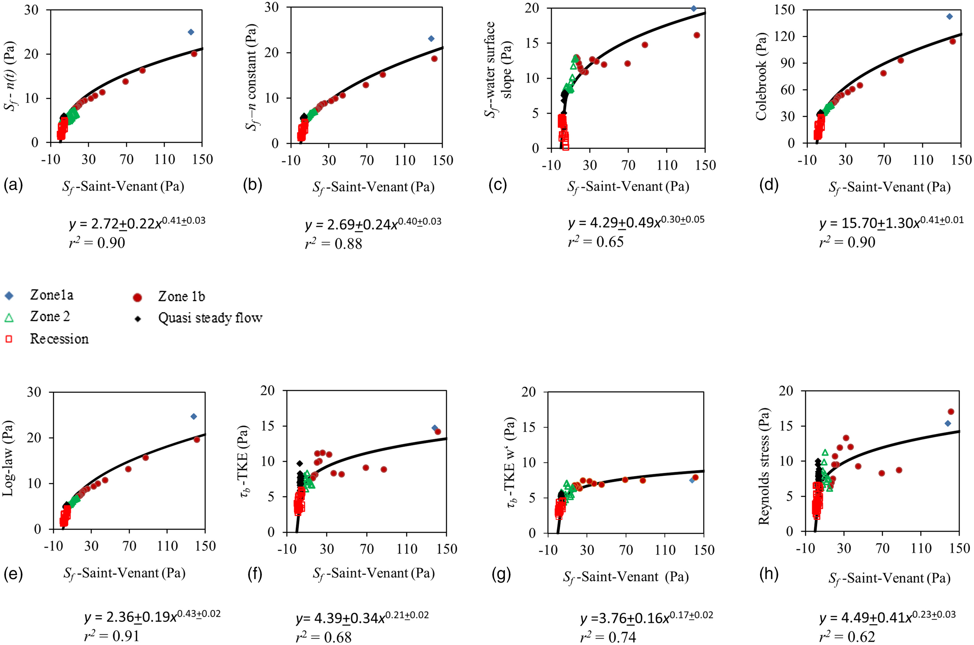
The other methods are advantageous in requiring less data and being less dependent on calculated derivates (which can be noisy), but have assumptions likely broken during these flows. Nonetheless, Fig. 6 shows that these other methods are all nonlinearly correlated with Sf-Saint-Venant for dry beds, including the higher stress portions, during which flow was more rapidly changing. This result suggests, at least empirically, that these simpler methods may be adapted or calibrated to give reasonable shear stress estimates during flash floods. Fig. 
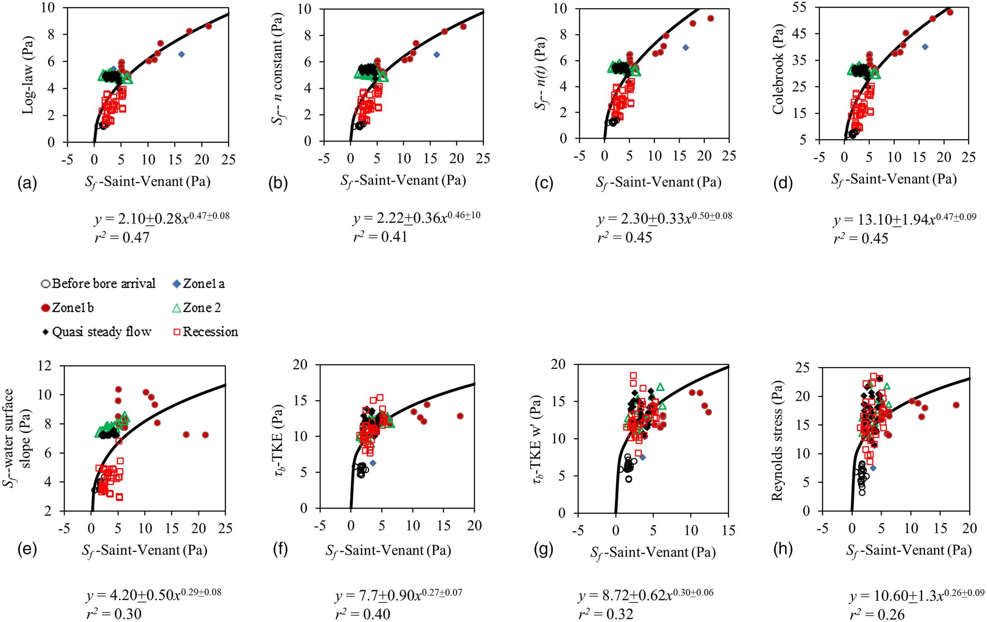
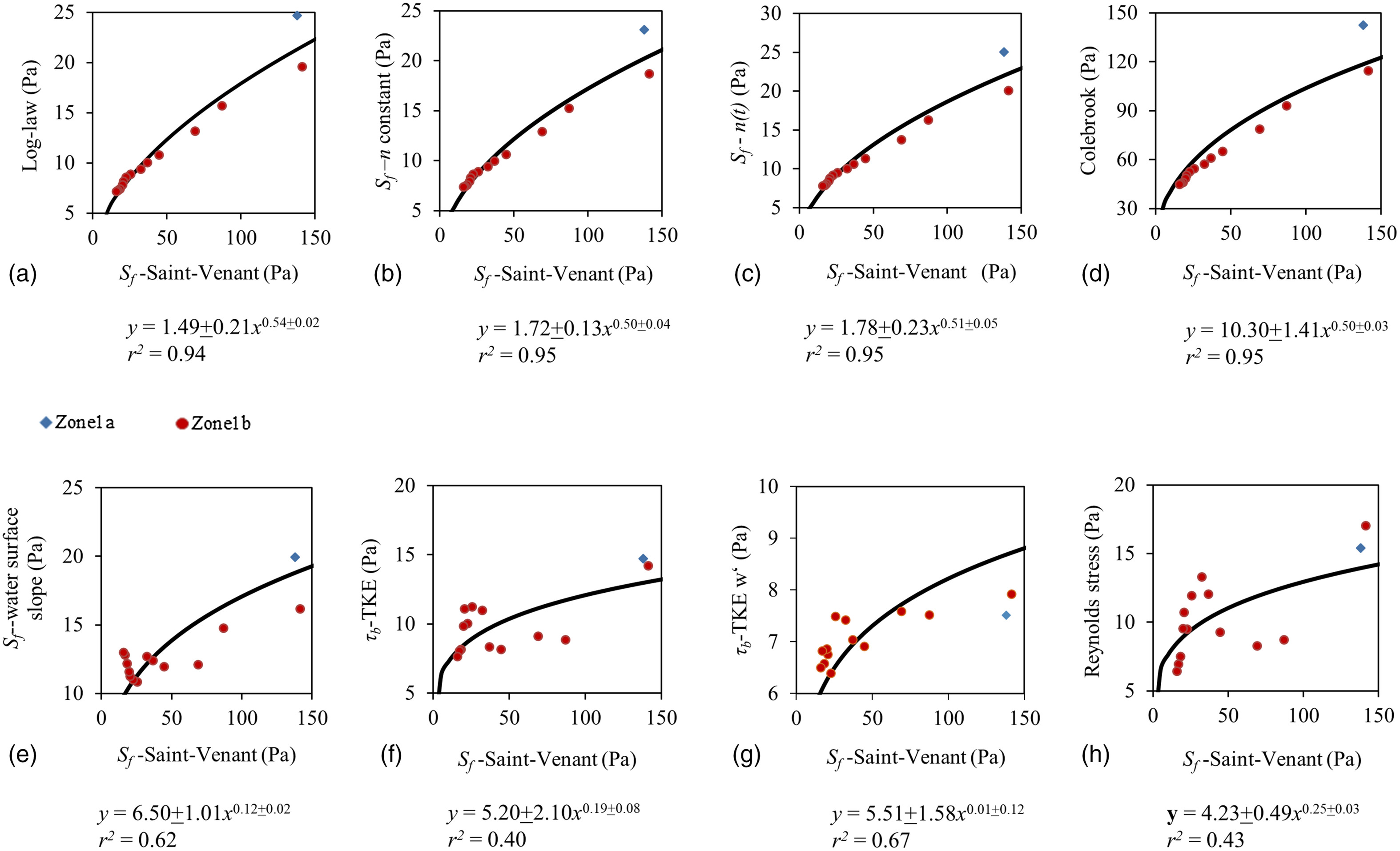
7 shows similar power-law scaling for wet-bed bores between the various methods and the Sf-Saint-Venant 
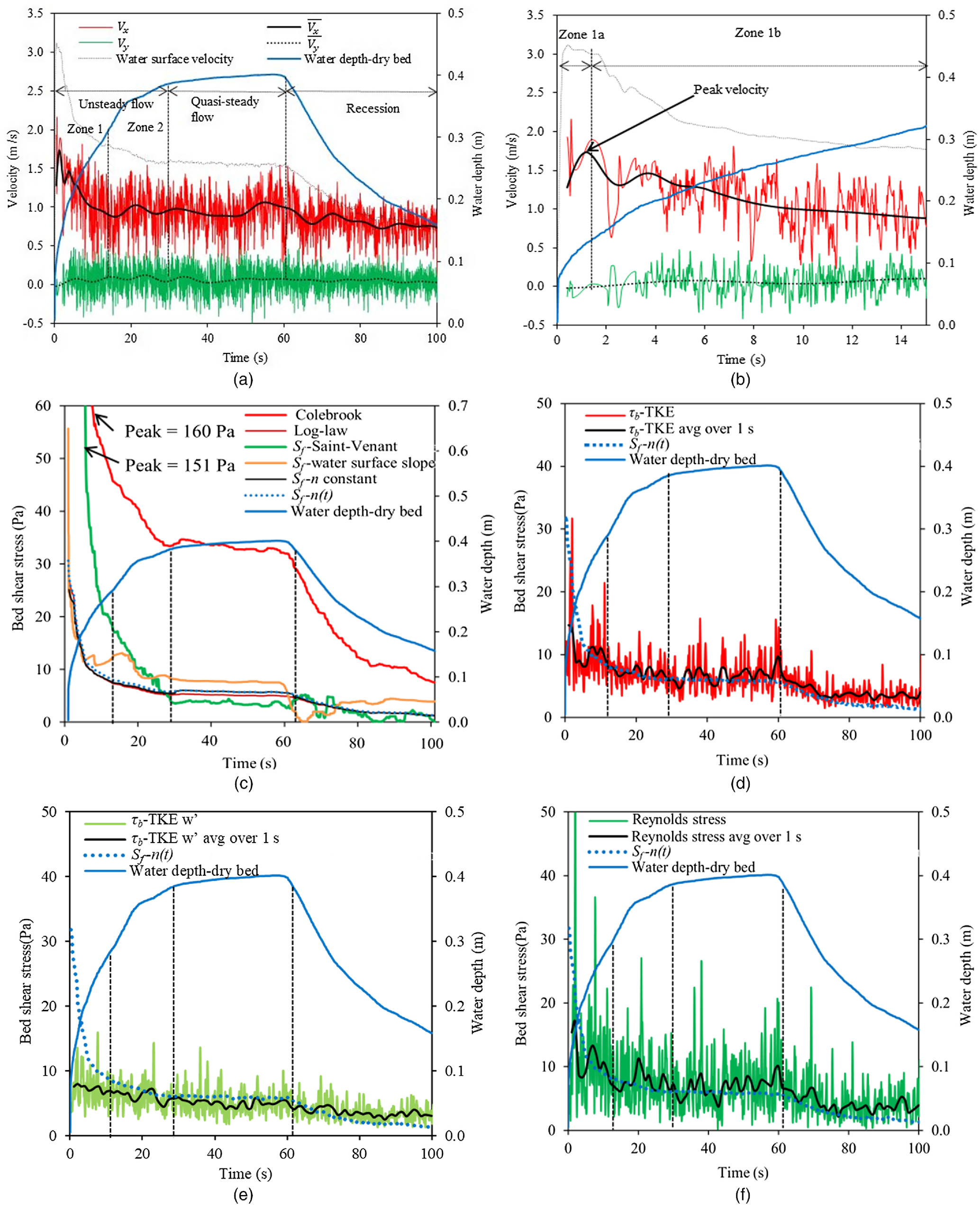
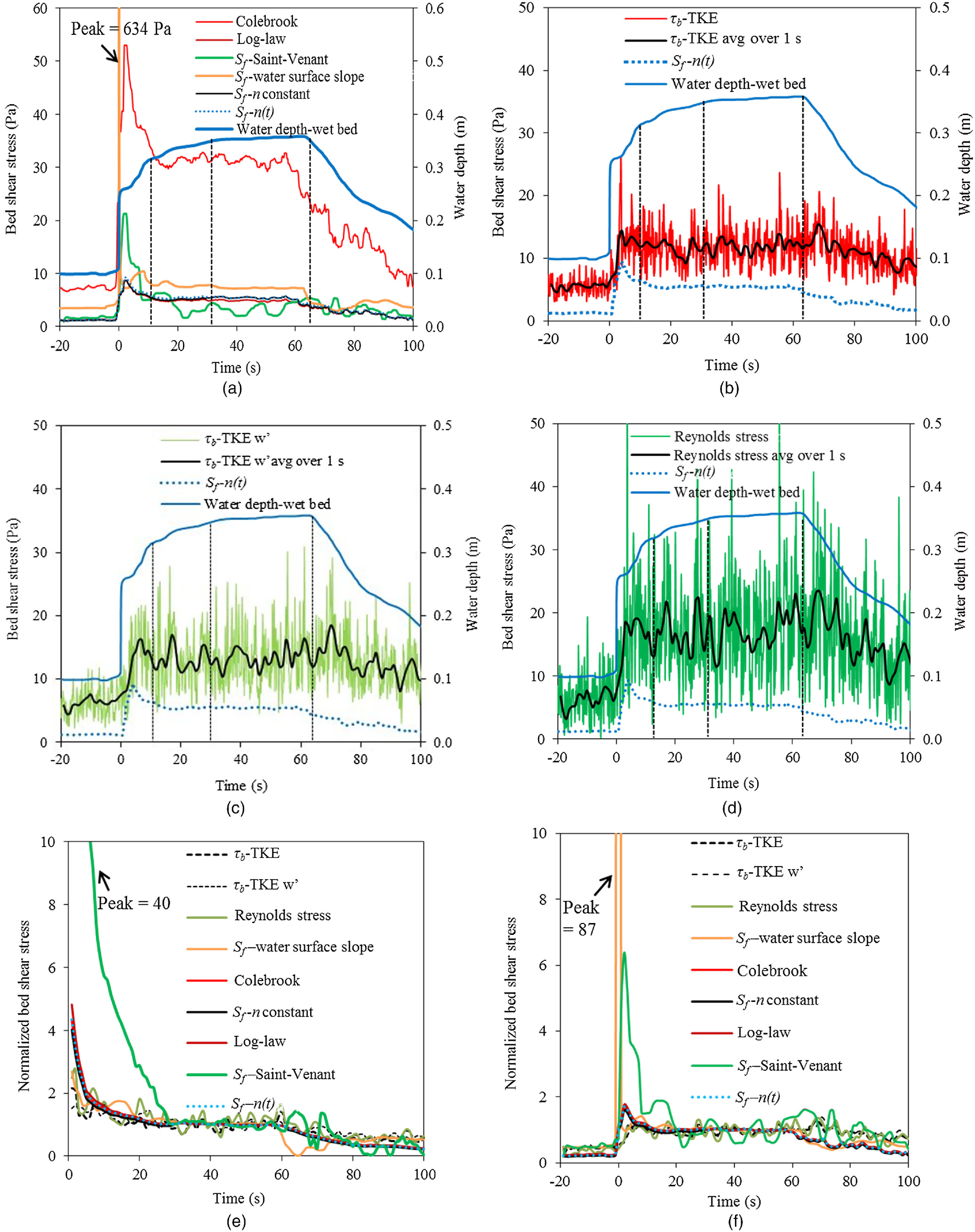
shear stresses. At the same time, for dry beds the peak Saint-Venant based shear stress was roughly 10 to 20 times larger than peak τb from other methods, and several times larger for wet bed conditions [Figs. 5(e and f)]. Methods that do not account for flow accelerations may underestimate stresses when flows are increasing rapidly.
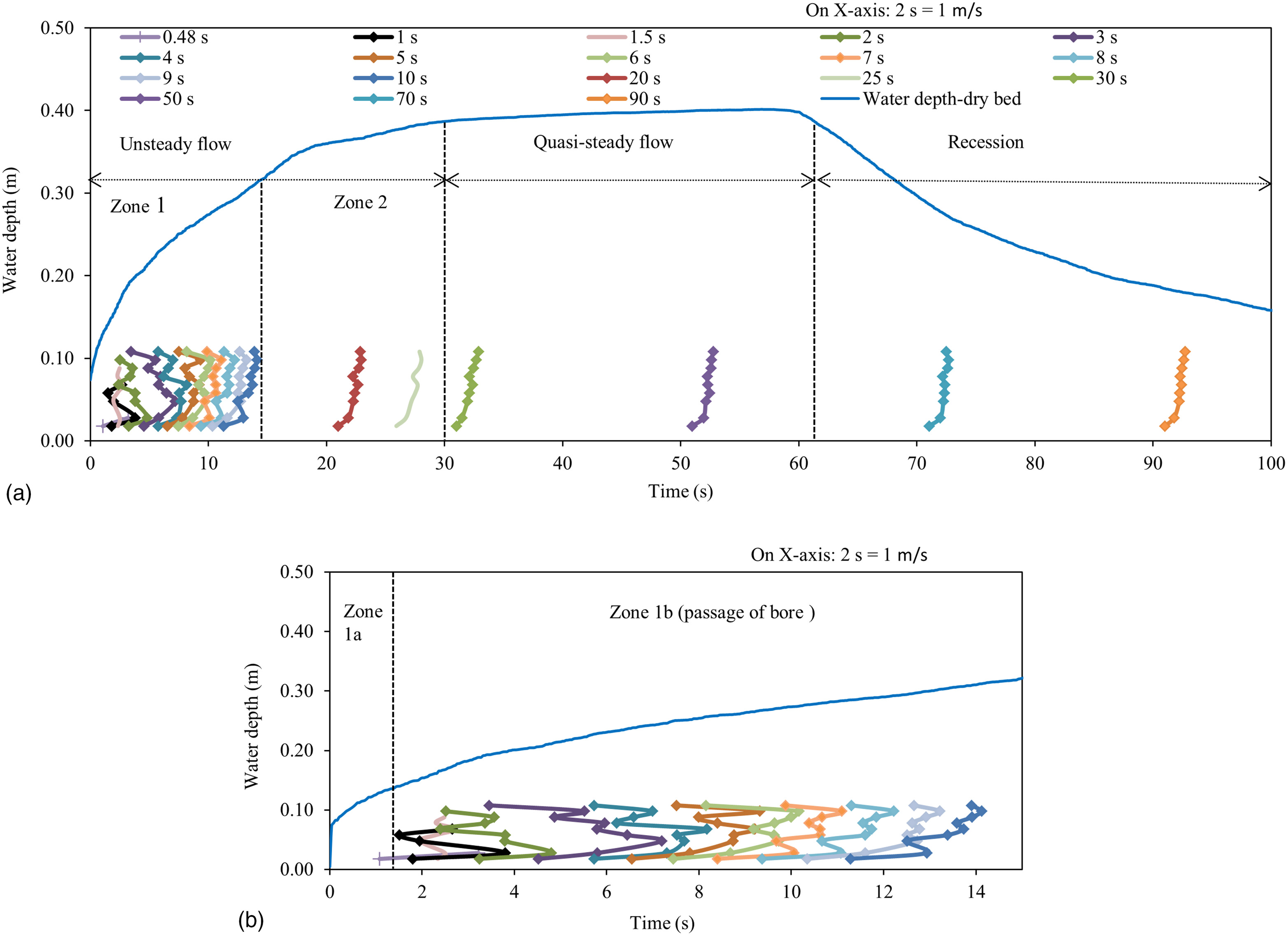
For dry bed flows, velocity profiles in the lower 10.8 cm of the water column rapidly transitioned from highly variable with height above the bed to more typical boundary-layer velocity profiles within the first 10  s, even as depth was still increasing and water surface slope was decreasing (Fig. 2). The assumption that a boundary layer has fully developed suggests that the Log-law method would be inappropriate for estimating shear stress for rapidly changing flows (Kikkert et al. 2012, 2013; O’Donoghue et al. 2016). However, in experiments with nonuniform flow accelerations, near-bed velocity profiles maintained their logarithmic form during both flow accelerations and decelerations (Song and Chiew 2001). The rapid development of velocity profiles while the bulk flow is still changing suggests that relations relating depth-averaged velocity to shear stress may be reasonable over a range of unsteady flow conditions.
In field settings, data quality is likely to be a challenge with many of these methods, and with Saint-Venant in particular. Even with significant averaging of dry-bed runs to reduce variability, the calculated derivatives tend to make our Saint-Venant τb calculations noisier than the methods that only use depth-averaged velocity [Figs. 4 and 5; Table 1; Eq. (S6)]. Water surface slope requires accurate spatio-temporal measurements of small changes in water surface elevation. For this reason, methods using depth and surface velocity time series may be less noisy than slope-based methods.
Lags between flow acceleration and changes in turbulence may explain why the turbulence-based methods predict much smaller peak shear stresses during dry bed bore arrival, and no peak τb for wet bed bore arrival. Comparing temporally accelerating pipe flow to steady pipe flow, He and Jackson (2000) found delays in turbulence production and propagation from the flow boundary to the middle of the flow. Decelerating flow similarly had a time lag, where turbulent velocity fluctuations remained higher than predicted based on the slowing velocity alone. Song and Chiew (2001) found similar lags for spatially accelerating and decelerating open channel flow. Relative to the other methods, these lags would predict reduced τb at and immediately after bore arrival for turbulence-based methods, as well as higher τb during recession. Although noisy, this pattern is generally observed [Figs. 5(e) and 6(f)]. For wet bed flows, we interpret that the lack of a turbulence-based peak τb after bore arrival occurred because it took several seconds for enhanced turbulence caused by shearing within the fluid at the interface between bore and flowing water (pre-bore flow depth 10  cm) to fully propagate to the bed.
Many studies demonstrate that instantaneous stresses associated with turbulent velocity fluctuations play a large role in forces on grains and sediment transport (e.g., Sumer et al. 2003; Schmeeckle et al. 2007). The lags embodied by the turbulence-derived shear stresses are physical. While turbulence contributes to the overall shear stress time series, we nonetheless interpret that these turbulence-based measures alone are incomplete representations of temporal shear stress changes. The empirical coefficients used in turbulence-based methods could vary with the degree and direction of unsteadiness (Pope 2000). In addition, we acknowledge potentially significant instrumental and methodological limitations of our ADV data. Conducting more than three experimental runs at a given ADV height would have reduced uncertainties in our turbulence-based calculations. Turbulent velocities in the first several seconds are challenging to measure because of aerated flow immediately after bore arrival (especially in the dry bed case), uncertainty from despiking, and separating the mean velocity from turbulence when the mean and variability are simultaneously changing. In field settings and during extreme events it is often impossible to measure near-bed turbulence; most instruments suitable for field turbulence measurements need to be in contact with the flow. Our experimental analysis usefully shows that turbulence-based methods suggest lower peak shear stresses at bore arrival, compared to other methods.
A key motivation for improving shear stress calculations in natural flash floods is to quantitatively predict sediment transport rates and channel changes. Our shear stresses predict that bedload flux would be highest immediately after bore arrival, and also higher during bore passage over a dry bed than that over a wet bed. Rapid scour and deposition are also hypothesized to be caused by bore passage. In the current analysis, correlations between shear stress methods allow different stress estimates to be predicted from each other. However, these regressions are specific to these experiments. Future studies could evaluate how well unsteadiness metrics can improve shear stress estimates during bores and similar rapidly changing flows, especially for applications where it is impossible to measure flow accelerations with sufficient accuracy to apply Saint-Venant models.

Conclusions

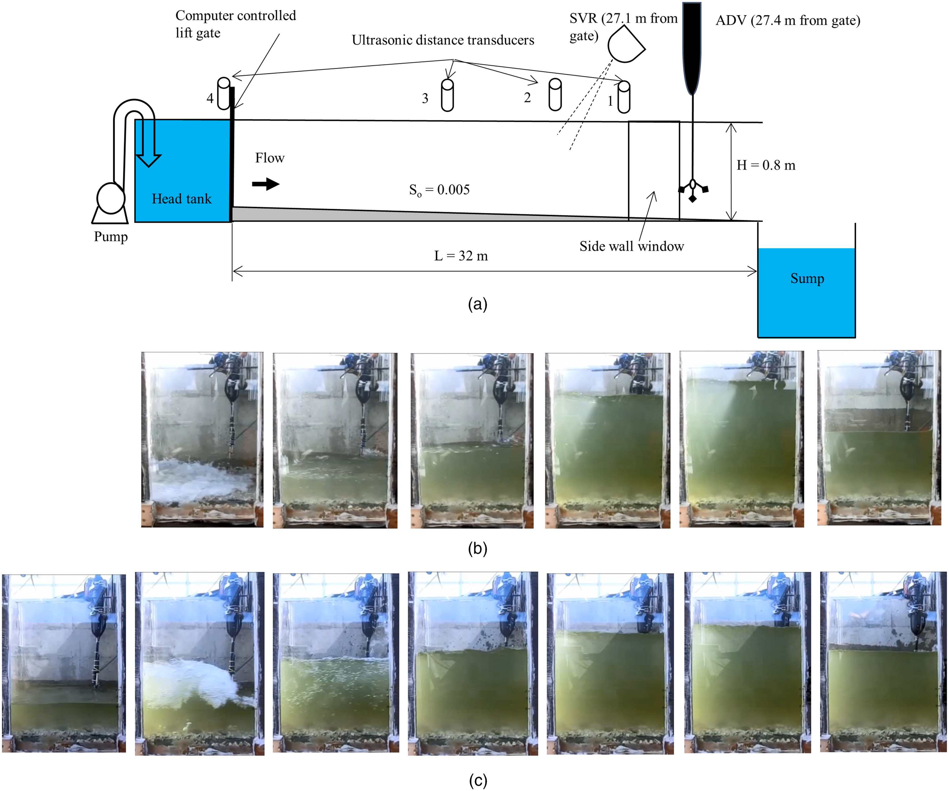
The objectives of the present study were to better understand flash flood bores by (1) comparing approaches for estimating bed shear stress in flash floods that could feasibly be applied in field settings; and (2) comparing shear stresses for bores arriving over both dry beds and over flowing water. We conducted experiments comparing flows propagating over rough dry beds (immobile gravel and concrete) and over shallowly flowing water. Bed shear stresses were calculated by nine previously proposed methods using a variety of data, including water depth, slope, depth-averaged velocity, and turbulent velocity fluctuation.
We have two main conclusions. First, the most theoretically justifiable method we evaluated is a version of the Saint-Venant equations for depth-averaged flow, which includes local flow accelerations in its force balance. During and immediately after bore arrival this method predicted consistently higher shear stresses than the other eight methods. However, because the Saint-Venant approach assumes that flow only varies gradually, our shear stress calculations at and immediately after bore arrival are likely inaccurate. The other eight methods we evaluated are commonly used in cases where steady flow can be assumed, and so may not apply to rapidly changing hydrographs. Nonetheless, using power-law regressions we found that these methods were all moderately to highly correlated with the Saint-Venant approach. While our regressions are specific to these experiments, the correlations suggest that it may be possible to empirically calculate reasonably accurate shear stresses soon after bore arrival. Turbulence-based methods for calculating shear stresses gave the lowest peak shear stresses in response to bore arrival, which we interpret to primarily be caused by time lags between mean flow accelerations and turbulence generation. Challenges of measuring and separating turbulent fluctuations from mean velocities during bores may also contribute to lower peak shear stresses using turbulence-based methods.
Second, we conclude that bores propagating over relatively shallow flowing water (1/3 to 1/4 of ultimate water depth) tend to have considerably lower peak shear stresses from bore arrival than do bores moving over dry beds, indicating the extent to which shallow water can dampen and dissipate near-bed shear stresses, even when overlying bores cause extremely sudden changes in depth and velocity.

Supplemental Materials

File (supplemental_material_jhend8.hyeng-13029_thappeta.zip)

Data Availability Statement

All data (Tables S1S3) used during the study are available in a repository online in accordance with funder data retention policies (Thappeta et al. 2021).

Acknowledgments

This project was funded by the Israel Science Foundation grant 834/14 and the NSF-BSF Grant 2018619 to JBL. The lead author was supported by a post-doctoral fellowship from the Ben Gurion University of the Negev Marcus Postdoctoral Fund. YS-P was in receipt of a Ben Gurion University of the Negev Kreitman postdoc fellowship. YS-P and JPLJ were also supported by The University of Texas at Austin Jackson School of Geosciences. The authors thank the reviewers and editors for their pertinent suggestions and comments.

References

Albayrak, I., and U. Lemmin. 2011. “Secondary currents and corresponding surface velocity patterns in a turbulent open-channel flow over a rough bed.” J. Hydraul. Eng. 137 (11): 1318–1334. https://doi.org/10.1061/(ASCE)HY.1943-7900.0000438.
Aleixo, R., S. Soares-Frazão, and Y. Zech. 2019. “Statistical analysis methods for transient flows—The dam-break case.” J. Hydraul. Res. 57 (5): 688–701. https://doi.org/10.1080/00221686.2018.1516700.
Biron, P. M., C. Robson, M. F. Lapointe, and S. J. Gaskin. 2004. “Comparing different methods of bed shear stress estimates in simple and complex flow fields.” Earth Surf. Processes Landforms 29 (11): 1403–1415. https://doi.org/10.1002/esp.1111.
Bombar, G. 2016. “Hysteresis and shear velocity in unsteady flows.” J. Appl. Fluid Mech. 9 (2): 839–853. https://doi.org/10.18869/acadpub.jafm.68.225.24454.
Briganti, R., N. Dodd, D. Pokrajac, and T. O’Donoghue. 2011. “Non linear shallow water modelling of bore-driven swash: Description of the bottom boundary layer.” Coastal Eng. 58 (6): 463–477. https://doi.org/10.1016/j.coastaleng.2011.01.004.
Cavaille, Y. 1965. “Contribution à l’étude de l’écoulement variable accompagnant la vidange brusque d’une retenue” [Contribution to the study of the variable flow accompanying the sudden emptying of a reservoir]. [In French.] In Vol. 410 of Publ. Scient. et Techn. du Ministère de l’Air, 165. Paris: French Ministry of Air.
Chanson, H. 2009. “Application of the method of characteristics to the dam break wave problem.” J. Hydraul. Res. 47 (1): 41–49. https://doi.org/10.3826/jhr.2009.2865.
Chanson, H., and N. J. Docherty. 2012. “Turbulent velocity measurements in open channel bores.” Eur. J. Mech. B Fluids 32 (Mar–Apr): 52–58. https://doi.org/10.1016/j.euromechflu.2011.10.001.
Chaudhry, M. H. 2008. Open channel flow: Unsteady flow. New York: Springer.
Chow, V. T. 1959. Open channel hydraulics. New York: McGraw-Hill.
Clauser, F. H. 1954. “Turbulent boundary layers in adverse pressure gradients.” J. Aeronaut. Sci. 21 (2): 91–108. https://doi.org/10.2514/8.2938.
Colebrook, C. F. 1939. “Turbulent flow in pipes, with particular reference to the transition region between the smooth and rough pipe laws.” J. Inst. Civ. Eng. 11 (4): 133–156. https://doi.org/10.1680/ijoti.1939.13150.
Czernuszenko, W., and P. M. Rowinski. 2008. “Shear stress statistics in a compound channel flow.” Arch. Hydro-Eng. Environ. Mech. 55 (1–2): 3–27.
Dey, S. 2014. Fluvial hydrodynamics: Hydrodynamic and sediment transport phenomena. Berlin: Springer.
Dey, S., R. Das, R. Gaudio, and S. K. Bose. 2012. “Turbulence in mobile-bed streams.” Acta Geophys. 60 (6): 1547–1588. https://doi.org/10.2478/s11600-012-0055-3.
Dey, S., and M. F. Lambert. 2005. “Reynolds stress and bed shear in nonuniform unsteady open-channel flow.” J. Hydraul. Eng. 131 (7): 610–614. https://doi.org/10.1061/(ASCE)0733-9429(2005)131:7(610).
Dressler, R. 1954. “Comparison of theories and experiments for the hydraulic dam-break wave.” Int. Assoc. Sci. Hydrol. 3 (38): 319–328.
Estrade, J. 1967. “Contribution à l’étude de la suppression d’un barrage. Phase initiale de l’écoulement” [Contribution to the study of the removal of a dam. Initial phase of flow]. [In French.] In Vol. 1 of Bulletin de la Direction des Etudes et Recherches, Series A, Nucléaire, Hydraulique et Thermique, 3–128. Chatou, France: Électricité de France Chatou.
Faure, J., and N. Nahas. 1961. “Etude numérique et expérimentale d’intumescences à forte courbure du front” [Numerical and experimental study of hydraulic bores with high front curvature]. [In French.] Houille Blanche 47 (5): 576–587. https://doi.org/10.1051/lhb/1961044.
Ghimire, B., and Z.-Q. Deng. 2011. “Event flow hydrograph-based method for shear velocity estimation.” J. Hydraul. Res. 49 (2): 272–275. https://doi.org/10.1080/00221686.2011.552463.
Goring, D. G., and V. I. Nikora. 2002. “Despiking acoustic Doppler velocimeter data.” J. Hydraul. Eng. 128 (1): 117–126. https://doi.org/10.1061/(ASCE)0733-9429(2002)128:1(117).
Graf, W. H., and T. Song. 1995. “Bed-shear stress in nonuniform and unsteady open-channel flows.” J. Hydraul. Res. 33 (5): 699–704. https://doi.org/10.1080/00221689509498565.
Gross, T. F., and A. R. M. Nowell. 1985. “Spectral scaling in a tidal boundary layer.” J. Phys. Oceanogr. 15 (5): 496–508. https://doi.org/10.1175/1520-0485(1985)015%3C0496:SSIATB%3E2.0.CO;2.
Haizhou, T., and W. H. Graf. 1993. “Friction in unsteady open-channel flow over gravel beds.” J. Hydraul. Res. 31 (1): 99–110. https://doi.org/10.1080/00221689309498863.
Hassan, M. A. 1990. “Observations of desert flood bores.” Earth Surf. Processes Landforms 15 (5): 481–485. https://doi.org/10.1002/esp.3290150512.
He, S., and J. D. Jackson. 2000. “A study of turbulence under conditions of transient flow in a pipe.” J. Fluid Mech. 408 (Apr): 1–38. https://doi.org/10.1017/S0022112099007016.
Henderson, F. M. 1963. “Flood waves in prismatic channels.” J. Hydraul. Div. 89 (4): 39–67. https://doi.org/10.1061/JYCEAJ.0000922.
Johnson, J. P. L., K. Delbecq, W. Kim, and D. Mohrig. 2016. “Experimental tsunami deposits: Linking hydrodynamics to sediment entrainment, advection lengths and downstream fining.” Geomorphology 253 (Jan): 478–490. https://doi.org/10.1016/j.geomorph.2015.11.004.
Khiadani, M. H., S. Beecham, J. Kandasamy, and S. Sivakumar. 2005. “Boundary shear stress in spatially varied flow with increasing discharge.” J. Hydraul. Eng. 131 (8): 705–714. https://doi.org/10.1061/(ASCE)0733-9429(2005)131:8(705).
Kikkert, G. A., T. O’Donoghue, D. Pokrajac, and N. Dodd. 2012. “Experimental study of bore-driven swash hydrodynamics on impermeable rough slopes.” Coastal Eng. 60 (1): 149–166. https://doi.org/10.1016/j.coastaleng.2011.09.006.
Kikkert, G. A., D. Pokrajac, T. O’Donoghue, and K. Steenhauer. 2013. “Experimental study of bore-driven swash hydrodynamics on permeable rough slopes.” Coastal Eng. 79 (Sep): 42–56. https://doi.org/10.1016/j.coastaleng.2013.04.008.
Kim, S.-C., C. T. Friedrichs, J. P.-Y. Maa, and L. D. Wright. 2000. “Estimating bottom stress in tidal boundary layer from acoustic Doppler velocimeter data.” J. Hydraul. Eng. 126 (6): 399–406. https://doi.org/10.1061/(ASCE)0733-9429(2000)126:6(399).
Koch, C., and H. Chanson. 2009. “Turbulence measurements in positive surges and bores.” J. Hydraul. Res. 47 (1): 29–40. https://doi.org/10.3826/jhr.2009.2954.
Lauber, G. 1997. “Experimente zur Talsperrenbruchwelle im glatten geneigten Rechteckkanal” [Experiments on the dam breach wave in a smooth inclined rectangular channel]. [In German.] Ph.D. thesis, Laboratory of Hydraulics, Hydrology and Glaciology, Swiss Federal Institute of Technology.
Leng, X., and H. Chanson. 2015. “Breaking bore: Physical observations of roller characteristics.” Mech. Res. Commun. 65 (Apr): 24–29. https://doi.org/10.1016/j.mechrescom.2015.02.008.
Leng, X., and H. Chanson. 2016. “Coupling between free-surface fluctuations, velocity fluctuations and turbulent Reynolds stresses during the upstream propagation of positive surges, bores and compression waves.” Environ. Fluid Mech. 16 (4): 695–719. https://doi.org/10.1007/s10652-015-9438-8.
Leng, X., and H. Chanson. 2017. “Unsteady velocity profiling in bores and positive surges.” Flow Meas. Instrum. 54 (Apr): 136–145. https://doi.org/10.1016/j.flowmeasinst.2017.01.004.
Liu, M., D. Zhu, and N. Najaratnam. 2002. “Evaluation of ADV measurements in bubbly two-phase flows.” In Proc., Hydraulic Measurements and Experimental Methods Conf. Reston, VA: ASCE.
López, F., and M. H. García. 1999. “Wall similarity in turbulent open-channel flow.” J. Hydraul. Eng. 125 (7): 789–796. https://doi.org/10.1061/(ASCE)0733-9399(1999)125:7(789).
MacVicar, B. J., E. Beaulieu, V. Champagne, and A. G. Roy. 2007. “Measuring water velocity in highly turbulent flows: Field test of an electromagnetic current meter (ECM) and an acoustic Doppler velocitmeter (ADV).” Earth Surf. Processes Landforms 32 (9): 1412–1432. https://doi.org/10.1002/esp.1497.
Mohajeri, S. H., A. Safarzadeh, and S. A. A. S. Neyshabouri. 2012. “A three tube pressure instrument for measuring the local bed shear stress in smooth and rough beds: Water infinitely deformable but still limited.” In Proc., 2nd IAHR Europe Congress. Madrid, Spain: International Association for Hydro-Environment Engineering and Research.
Moore, A. L., B. G. McAdoo, and A. Ruffman. 2007. “Landward fining from multiple sources in a sand sheet deposited by the 1929 Grand Banks tsunami, Newfoundland.” Sediment. Geol. 200 (3–4): 336–346. https://doi.org/10.1016/j.sedgeo.2007.01.012.
Mrokowska, M. M., P. M. Rowinski, and M. B. Kalinowska. 2015a. “Evaluation of friction velocity in unsteady flow experiments.” J. Hydraul. Res. 53 (5): 659–669. https://doi.org/10.1080/00221686.2015.1072853.
Mrokowska, M. M., P. M. Rowinski, and M. B. Kalinowska. 2015b. “A methodological approach of estimating resistance to flow under unsteady flow conditions.” Hydrol. Earth Syst. Sci. 19 (10): 4041–4053. https://doi.org/10.5194/hess-19-4041-2015.
Nezu, I., A. Kadota, and H. Nakagawa. 1997. “Turbulent structure in unsteady depth-varying open channel flows.” J. Hydraul. Eng. 123 (9): 752–763. https://doi.org/10.1061/(ASCE)0733-9429(1997)123:9(752).
Nikora, V., and D. Goring. 2000. “Flow turbulence over fixed and weakly mobile gravel beds.” J. Hydraul. Eng. 126 (9): 679–690. https://doi.org/10.1061/(ASCE)0733-9429(2000)126:9(679).
O’Donoghue, T., G. A. Kikkert, D. Pokrajac, N. Dodd, and R. Briganti. 2016. “Intra-swash hydrodynamics and sediment flux for dambreak swash on coarse-grained beaches.” Coastal Eng. 112 (Jun): 113–130. https://doi.org/10.1016/j.coastaleng.2016.03.004.
Pope, N. D., J. Widdows, and M. D. Brinsley. 2006. “Estimation of bed shear stress using the turbulent kinetic energy approach—A comparison of annular flume and field data.” Cont. Shelf Res. 26 (8): 959–970. https://doi.org/10.1016/j.csr.2006.02.010.
Pope, S. 2000. Turbulent flow. New York: Cambridge University Press.
Reid, I., D. M. Powell, J. B. Laronne, and C. Garcia. 1994. “Flash floods in desert rivers: Studying the unexpected.” Eos Trans. Am. Geophys. Union 75 (39): 452. https://doi.org/10.1029/94EO01076.
Rowinski, P. M., W. Czernuszenko, and J. M. Marc. 2000. “Time dependent shear velocities in channel routing.” Hydrol. Sci. J. 45 (6): 881–895. https://doi.org/10.1080/02626660009492390.
Schmeeckle, M. W., J. M. Nelson, and R. L. Shreve. 2007. “Forces on stationary particles in near-bed turbulent flows.” J. Geophys. Res.: Earth Surf. 112 (F2): F02003. https://doi.org/10.1029/2006JF000536.
Schoklitsch, A. 1917. “Uber Dambruchwellen” [Over dam break waves]. [In German.] In Vol. 126 of Kaiserliche Akademie der Wissenschaften, Wien, Mathematisch-Naturwissenschaftliche Klasse, Sitzungberichte IIa, 1489–1514. Vienna, Austria: K.K. Hof and the State Printer.
Shen, Y., and P. Diplas. 2010. “Modeling unsteady flow characteristics of hydropeaking operations and their implications on fish habitat.” J. Hydraul. Eng. 136 (12): 1053–1066. https://doi.org/10.1061/(ASCE)HY.1943-7900.0000112.
Song, T., and Y. M. Chiew. 2001. “Turbulence measurement in nonuniform open-channel flow using acoustic Doppler velocimeter (ADV).” J. Eng. Mech. 127 (3): 219–232. https://doi.org/10.1061/(ASCE)0733-9399(2001)127:3(219).
Song, T., and W. H. Graf. 1996. “Velocity and turbulence distribution in unsteady open-channel flows.” J. Hydraul. Eng. 122 (3): 141–154. https://doi.org/10.1061/(ASCE)0733-9429(1996)122:3(141).
Soulsby, R. L. 1983. Physical oceanography of coastal and shelf seas, 189–266. Amsterdam, Netherlands: Elsevier. https://doi.org/10.1016/S0422-9894(08)70503-8.
Stapleton, K. R., and D. A. Huntley. 1995. “Seabed stress determinations using the inertial dissipation method and the turbulent kinetic energy method.” Earth Surf. Processes Landform 20 (9): 807–815. https://doi.org/10.1002/esp.3290200906.
Sumer, B. M., L. H. C. Chua, N.-S. Cheng, and J. Fredsøe. 2003. “Influence of turbulence on bed load sediment transport.” J. Hydraul. Eng. 129 (8): 585–596. https://doi.org/10.1061/(ASCE)0733-9429(2003)129:8(585).
Swamee, P. K., and A. K. Jain. 1976. “Explicit equations for pipe-flow problems.” J. Hydraul. Div. 102 (5): 657–664. https://doi.org/10.1061/JYCEAJ.0004542.
Tamari, S., F. Garcia, J. I. Arciniega-Ambrocio, and A. Porter. 2013. Laboratory and field testing of a handheld radar to measure the water velocity at the surface of open channels. Jiutepec, Mexico: Mexican Institute of Water Technology.
Thappeta, S. K., J. P. L. Johnson, E. Halfi, Y. S. Peretz, Y. Storz, and J. B. Laronne. 2021. Supplemental materials for: Bed shear stress in experimental flash flood bores over dry beds and over flowing water: A comparison of methods. Cambridge, MA: Figshare. https://doi.org/10.6084/m9.figshare.15067050.v2.
Welber, M., J. L. Coz, J. B. Laronne, G. Zolezzi, D. Zamler, G. Dramais, A. Hauet, and M. Salvaro. 2016. “Field assessment of noncontact stream gauging using portable surface velocity radars (SVR).” Water Resour. Res. 52 (2): 1108–1126. https://doi.org/10.1002/2015WR017906.

Information & Authors

Information

Published In

Go to Journal of Hydraulic Engineering
Journal of Hydraulic Engineering
Volume 149Issue 4April 2023

History

Received: Aug 1, 2021
Accepted: Sep 1, 2022
Published online: Jan 19, 2023
Published in print: Apr 1, 2023
Discussion open until: Jun 19, 2023

Authors

Affiliations

Assistant Professor, Dept. of Civil Engineering, Visvesvaraya National Institute of Technology, Nagpur, Maharashtra 440010, India; Postdoctoral Researcher, Dept. of Geography and Environmental Development, Ben-Gurion Univ. of the Negev, Beer Sheva 84105, Israel (corresponding author). ORCID: https://orcid.org/0000-0002-1170-3129. Email: [email protected]; [email protected]
Joel P. L. Johnson [email protected]
Associate Professor, Dept. of Geological Sciences, Univ. of Texas at Austin, Austin, TX 78712. Email: [email protected]
Hydrologist, Desert Floods Research Center, Dead Sea and Arava Science Center, Masada 94335, Israel; Postdoctoral Researcher, Dept. of Geography and Environmental Development, Ben-Gurion Univ. of the Negev, Beer Sheva 84105, Israel. ORCID: https://orcid.org/0000-0002-4045-2824. Email: [email protected]
Yael Storz Peretz [email protected]
Israel Water Authority, Israel Hydrological Service, Jerusalem 9103401, Israel. Email: [email protected]
Professor Emeritus, Dept. of Geography and Environmental Development, Ben-Gurion Univ. of the Negev, Beer Sheva 84105, Israel. ORCID: https://orcid.org/0000-0002-2889-9316. Email: [email protected]

Metrics & Citations

Metrics

Citations

Download citation

If you have the appropriate software installed, you can download article citation data to the citation manager of your choice. Simply select your manager software from the list below and click Download.

View Options

Media

Figures

Other

Tables

Share

Share

Copy the content Link

Share with email

Email a colleague

Share