Cyclic Hysteretic Behavior and Development of the Secant Shear Modulus of Sand under Drained and Undrained Conditions
Publication: International Journal of Geomechanics
Volume 24, Issue 7
Abstract
The secant shear modulus is an important parameter in several geotechnical engineering models and calculation approaches. The characteristics of this parameter are very complex due to the hysteretic behavior of cyclically loaded soils. Its characteristics primarily depend on the mean effective confining stress and the void ratio. In this paper, the characteristics of the secant shear modulus of sand under large shear strain amplitude are investigated in detail based on the results of several cyclic triaxial and simple shear tests under drained and undrained conditions. The evaluation of the secant shear modulus based on the shape of the open stress–strain hysteresis loop is then discussed. Under certain loading conditions, the secant shear modulus defined from the reloading and unloading branches of the loop obviously differ. The evolution of the stiffness index, which measures the change in the secant shear modulus due to cyclic loading, shows that the drainage conditions play an essential role in the behavior of the secant shear modulus.
Introduction
There are two different definitions of shear modulus: (1) the tangential shear modulus, representing the slope of the stress–strain curve at a given point; and (2) the secant shear modulus, indicating the slope of the stress–strain hysteresis loop. In general, the shear modulus is denoted by the capital letter G. In the following sections, only the secant shear modulus is considered and is denoted by Gs.
Different test methods and procedures have been developed in recent years to evaluate the secant shear modulus. The most commonly used laboratory tests for determining the dynamic and cyclic soil stiffness parameters include resonant column, simple shear, and triaxial tests. Fig. 1 defines the secant shear modulus, Gs, for ideal cyclic strain-controlled simple shear test conditions. The figure schematically shows the hysteresis cyclic loops of the first cycle, N = 1, and further cycles, N > 1. According to several investigations, Gs can be obtained as the slope of the straight line between the center and the tips of the loop (Fig. 1) or between the two tips of the loop (Vucetic and Dobry 1991; Vucetic 1994; Vucetic and Tabata 2003; Vucetic et al. 2021; Silver and Seed 1969; Park and Silver 1975; Song et al. 2004; Seed et al. 1986). For extremely small cyclic shear strain amplitudes (γampl < 10−6), the secant shear modulus approaches its maximum value and is identical to the theoretical value of the maximum tangential shear modulus Gmax. The maximum tangential shear modulus is evaluated as the tangent at the starting point of the initial backbone curve or as the tangent at the reversal points of the unloading and reloading branches of the loop. The backbone curve is the stress–strain curve of the monotonic first loading from the initial state, and the negative part is an extension of the initial curve along the negative direction. These definitions of the secant shear modulus are applicable under the condition of a perfectly closed hysteresis loop, except for the first cycle with the initial loading branch. In a closed cyclic loop, there is no difference in the secant shear modulus between the unloading and reloading branches. However, the hysteresis loop is not always closed. This results in different secant modulus values for the unloading and reloading branches. It is therefore necessary to investigate the secant modulus in more detail.

Based on the results of the triaxial and simple shear tests, the main objectives of this paper are to determine the characteristics of the secant shear modulus of sand at large cyclic strain amplitudes within the nonlinear plastic range under drained and undrained conditions. The differences in the secant moduli between unloading and reloading by different forms of the hysteresis loop are examined. Furthermore, the evolution of the stiffness index, which measures the change in the secant shear modulus due to cyclic loading, is another objective of the study.
In the following sections, the definitions of the stress and strain conditions in the triaxial and simple shear tests and the definition of the secant shear modulus through unloading and reloading for different forms of the hysteresis loop are presented. The testing programs, procedures, and materials are presented in the following section. Furthermore, the behavior and development of the secant shear modulus regarding different loading and drainage conditions are discussed.
Theoretical Background
Stress and Strain Conditions in Triaxial and Simple Shear Tests
In this study, cyclic triaxial and simple shear tests are utilized to evaluate the secant shear modulus of sand. In this section, the definitions of the stress and strain states in these tests are presented.
In the triaxial test, the axial and radial effective stress components can be described with σ1 and σ3, respectively (Fig. 2). The prime for expressing the effective stress is omitted in the following sections. With a cylindrical specimen, the stress and strain conditions are rotationally symmetric. The stress condition can be expressed with the Roscoe invariants mean stress p and deviatoric stress q as follows:
(1)

In the p–q plane, the stress state can be described with the stress ratio η = q/p (Fig. 3). For isotropic consolidation, η = 0. In the critical state, this stress ratio is ηc for compression and ηe for extension. The inclination of the critical state lines ηc and ηe can be calculated from the friction angle φc. After consolidation, a cyclic loading component qampl is applied to the specimen under average stress conditions pav and qav. The specimen deformation can be described with the axial strain ɛ1 and the radial strain ɛ3 (Fig. 2). The axial strain ɛ1 is evaluated directly from the measurement of the axial displacement. The radial strain ɛ3 is measured with a local displacement transducer (Wichtmann 2016; Goto et al. 1991) or calculated from the measured volumetric strain as . The common invariants of the strain components are the deviatoric strain ɛq and the shear strain γ with
(2)

The secant shear modulus Gs in the triaxial test can be defined as follows:with the increment in the deviatoric stress Δq = 2qampl = (qmax − qmin) and the increment in the deviatoric strain . In several studies, the increments Δq and Δɛq have also been referred to as double amplitudes. As an alternative to this calculation method, the secant shear modulus Gs can be estimated from Young's modulus E and Poisson's ratio ν, as follows:
(3)
(4)
This alternative method does not require measurement of the radial strain or volumetric strain. However, Poisson's ratio ν must be assumed. In undrained tests, Poisson's ratio is ν = 0.5, while in drained tests with sand, Poisson's ratio ν ranges from 0.20 to 0.40 (Wichtmann and Triantafyllidis 2009). Due to uncertainties in the estimation of Poisson's ratio, the authors prefer the calculation method according to Eq. (3). The difference between these two calculation methods is discussed in the Appendix.
Fig. 3 shows three possible initial stress states during the cyclic triaxial test: (I) compression; (II) isotropic conditions; and (III) extension. Under these conditions, the typical forms of the hysteresis loop are also presented in the figure. The definitions of the secant shear modulus in these cases differ and are explained in the following section.
Simple shear is defined as the vertical rectangular cross section deforming into a parallelogram during shearing, while the cross section in the horizontal plane remains unchanged. The stress and strain states of the simple shear test are shown in Fig. 2. In the most common type of simple shear device, only the normal and shear forces on the top surface of the specimen (σv and τ, respectively) can be measured. The complementary normal and shear stresses (σh and τ, respectively) on the side surface cannot be measured and are therefore unknown. The volumetric strain is identical to the axial strain ɛv = ɛa. Under this condition, the specimen deformation can be described with the axial strain ɛa and the shear strain γ, which is determined from the measured displacement of the top cap and the initial height of the specimen. The secant shear modulus Gs is calculated from the shear stress amplitude τampl = (τmax – τmin)/2 and the shear strain amplitude γampl = (γmax – γmin)/2 as follows:
(5)
Different Forms of Hysteresis Loops and Definition of the Secant Shear Modulus
Depending on the stress and loading conditions, a hysteresis loop can have different shapes. Therefore, a universal definition of secant shear modulus Gs does not exist. The problem of a nonclosed hysteresis loop is well known and has been mentioned in several studies (Wichtmann 2005; Glasenapp 2016; Wichtmann 2016; Le 2015). However, the determination of the secant shear modulus in these cases has not been clearly defined. In addition, in the current ASTM standards for simple shear and triaxial tests, a recommendation for the evaluation of Gs is missing, according to ASTM D8296-19 (ASTM 2019) ASTM D3999-1991 (Reapproved 2003) (ASTM 2003). In this section, the definitions of the secant shear moduli for the different forms of the hysteresis loop used in this study are presented.
In a perfectly closed hysteresis loop, the start and end points are identical (Fig. 1). The secant shear moduli calculated from the unloading and reloading branches are the same. However, under cyclic loading with large strains, the specimen is expected to undergo permanent deformation. The cyclic loop in these tests does not close. Depending on the loading conditions, a wide open hysteresis loop may occur (Fig. 3, Cases I and III). In these cases, the secant shear moduli for unloading and reloading must be separately evaluated.
In laboratory tests, cyclic loads are usually applied in the form of a combination of the static component and the harmonic oscillation component of the load. The static and oscillation components of the harmonic load are denoted by subscripts av and ampl, respectively. Under symmetric loading, the static load is zero (two-way loading). If the sign of the load remains unchanged during the test, it is referred to as one-way loading. The secant shear modulus for different forms of hysteresis loops is defined through example triaxial tests (Fig. 4). Figs. 4(a and d) show different oscillation components of the deviatoric stress qampl (Load cases I and II, respectively). In both cases, the deviatoric stress develops according to a sinusoidal curve with the same magnitude and frequency but with a π/2 phase shift. This suggests that the deviatoric stress qampl starts along the positive direction in Load case I [Fig. 4(a)] and along the negative direction in Load case II [Fig. 4(d)]. In Fig. 4, the first cycle is presented with a solid line, and the second cycle is presented with a dashed line. According to Load cases I and II, the hysteresis loops of the first and second cycles are presented under symmetrical two-way loading with qav = 0 kPa [Figs. 4(b and e)] and under one-way loading with qav = 100 kPa [Figs. 4(c and f)]. In Load case I, the secant modulus calculated from the extreme points of the loop is the value of the unloading branch, . In Load case II, the secant modulus between the extreme points is the value of the reloading branch, . Considering this difference, the reloading modulus in Case I is defined based on the last quarter of the first cycle and the first quarter of the following cycle. is calculated as the inclination of the line between Extreme points B and C. Similarly, to evaluate the unloading modulus in Case II, Extreme points B and C are used. The turning point is not always clearly identifiable [Fig. 4(c), Point A]. In this case, the extreme point, defined as the tip of the loop according to Vucetic (1988), Mortezaie and Vucetic (2012), is used to calculate the modulus. In the simple shear tests, the evaluation procedures for the loading and unloading secant shear moduli are analogous.

Stiffness Index
To describe the reduction in the secant shear modulus with the variation in the shear strain amplitude γampl, normalized values Gs/Gmax are commonly used (Hardin and Drnevich 1972; Bai 2010; Wichtmann and Triantafyllidis 2013; Doroudian and Vucetic 1995; Kukusho 1980). Similarly, to quantify the development of Gs versus the number of cycles N during laboratory tests in large strain ranges, the concept of the stiffness index was proposed by Idriss et al. (1978). This index is defined as the normalization of the secant shear modulus with the modulus of the first cycle:
(6)
In cyclic tests within a large strain range, excess pore-water pressure or a change in density is expected. This can lead to a change in the secant shear modulus during the test. The stiffness index starts at δ = 1, expresses the variation in the shear modulus in relation to the initial value, and is called cyclic degradation.
Testing Programs
Materials
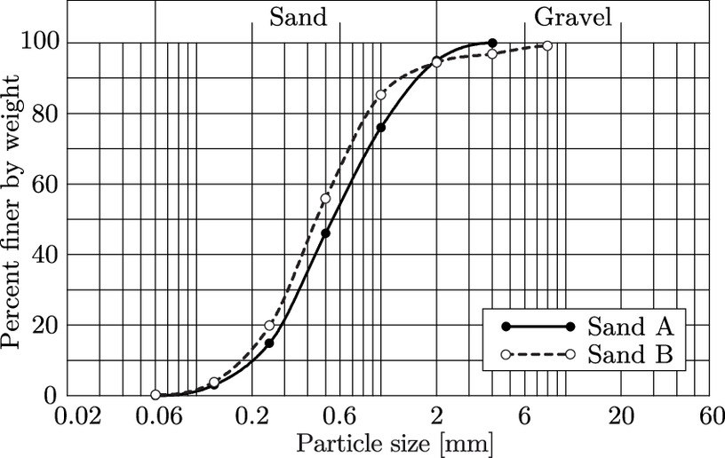
The grain size distributions of the two sands tested in the present study are shown in Fig. 5. Sand A is a medium to coarse-grained sand originating from an excavation pit in northern Berlin. Sand B is also a medium to coarse-grained sand retrieved from another location in Berlin. Light microscopy images showed that these two sands exhibit a rounded grain shape (Glasenapp 2016). The soil mechanical characteristics of the tested sands are listed in Table 1. Further characteristics and standard test results for these sands can be found in Glasenapp (2016), Le (2015), and Bai (2010).
Equipments and Procedures
In the experimental investigations in this study, a simple shear device and two triaxial devices were used. The first cyclic triaxial device used a hydraulic driving system for axial load application and pneumatic controllers for cell and back pressure application. The volume was measured using a burette system, allowing an accurate measurement of the volume change during the test. This device was used to perform the tests under drained conditions with up to 100,000 cycles. More details on this triaxial device can be found in Le (2015). The second triaxial device used in this study was a device with an electromechanical driving system for cyclic axial load application. The back and cell pressures in this device were applied by two pressure controllers. These controllers were simultaneously used for volume measurement. The second triaxial device was more suitable for undrained tests with a significantly smaller number of cycles than for drained tests. The construction and technical details of this device were presented by Glasenapp (2016). All specimens for the triaxial tests exhibit the same diameter and height of D × H = 100 × 200 mm. The test materials were prepared by dry pluviation and then saturated under a back pressure of 300 kPa. The saturation degree was evaluated with the B value, according to Skempton (1954). All of the tests in this study yielded a B-value > 0.95.
In addition to the triaxial devices, an electromechanical cyclic simple shear device of the modified NGI type was used in this study. This test device could perform monotonic and cyclic loading with different boundary conditions: constant normal stress (drained condition) and constant volume (undrained condition). Furthermore, specimens of different sizes could be tested. In this study, a specimen diameter of 9 cm with a height of 2 cm was preferred. The construction and technical details of this device were presented by Le and Rackwitz (2020). As in the triaxial tests, the materials were prepared via dry pluviation. All simple shear tests were conducted with dry specimens. Undrained conditions were ensured via dry specimens with a constant-volume controller. The simple shear test procedure in this study was in accordance with ASTM D8296-19 (ASTM 2019).
Programs
The main focus of the study is the investigation of the characteristics and evolution of the secant shear modulus during cyclic loading considering the drainage condition and form of the hysteresis loop. Regarding these aims, cyclic triaxial and simple shear tests were conducted employing two sands under different stress and drainage conditions. The test programs are presented in Tables 2–4.
| No. | Material | pav (kPa) | qav (kPa) | qampl (kPa) | Condition | Cycles | Initial relative density ID0 (%) | Remark |
|---|---|---|---|---|---|---|---|---|
| TX1 | Sand A | 200 | 150 | 40 | Drained | 1,000 | 59 | — |
| TX2 | Sand A | 200 | 150 | 40 | Undrained | 1,000 | 74 | — |
| TX3 | Sand A | 200 | 0 | 20 | Undrained | 2,292 | 71 | — |
| TX4 | Sand A | 200 | 0 | 40 | Undrained | 40 | 70 | — |
| TX5 | Sand A | 200 | 0 | 60 | Undrained | 5 | 72 | — |
| TX6 | Sand A | 200 | 0 | 40 | Undrained | 25 | 73 | With 1 precycle |
| TX7 | Sand A | 200 | 150 | 20 | Undrained | 1,000 | 71 | — |
| TX8 | Sand A | 200 | 150 | 40 | Undrained | 1,000 | 74 | — |
| TX9 | Sand A | 200 | 150 | 60 | Undrained | 1,000 | 71 | — |
| TX10 | Sand A | 200 | 150 | 80 | Undrained | 1,000 | 70 | — |
| No. | Material | σv (kPa) | τav (kPa) | τampl (kPa) | Condition | Cycles | Initial relative density ID0 (%) |
|---|---|---|---|---|---|---|---|
| SS1 | Sand A | 200 | 0 | 30 | Drained | 10,000 | 65 |
| SS2 | Sand A | 200 | 10 | 30 | Drained | 10,000 | 64 |
| SS3 | Sand A | 200 | 20 | 30 | Drained | 10,000 | 63 |
| SS4 | Sand A | 200 | 30 | 30 | Drained | 10,000 | 63 |
| SS5 | Sand A | 200 | 40 | 30 | Drained | 10,000 | 64 |
| SS6 | Sand A | 200 | 50 | 30 | Drained | 10,000 | 63 |
| SS7 | Sand A | 200 | 60 | 30 | Drained | 10,000 | 66 |
| SS8 | Sand A | 200 | 70 | 30 | Drained | 10,000 | 63 |
| SS9 | Sand B | 150 | 0 | 7,5 | Drained | 1,000 | 61 |
| SS10 | Sand B | 150 | 0 | 10 | Drained | 1,000 | 66 |
| SS11 | Sand B | 150 | 0 | 15 | Drained | 1,000 | 65 |
| SS12 | Sand B | 150 | 0 | 20 | Drained | 1,000 | 64 |
| SS13 | Sand B | 150 | 0 | 5 | Drained | 1,000 | 43 |
| SS14 | Sand B | 150 | 0 | 7,5 | Drained | 1,000 | 43 |
| SS15 | Sand B | 150 | 0 | 10 | Drained | 1,000 | 43 |
| SS16 | Sand B | 150 | 0 | 15 | Drained | 1,000 | 42 |
| SS17 | Sand B | 150 | 0 | 7,5 | Undrained | 159 | 65 |
| SS18 | Sand B | 150 | 0 | 10 | Undrained | 49 | 65 |
| SS19 | Sand B | 150 | 0 | 15 | Undrained | 21 | 62 |
| SS20 | Sand B | 150 | 0 | 20 | Undrained | 11 | 63 |
| SS21 | Sand B | 150 | 0 | 5 | Undrained | 480 | 42 |
| SS22 | Sand B | 150 | 0 | 7,5 | Undrained | 93 | 43 |
| SS23 | Sand B | 150 | 0 | 10 | Undrained | 31 | 39 |
| SS24 | Sand B | 150 | 0 | 15 | Undrained | 7 | 41 |
| No. | Material | σv (kPa) | γav (%) | γampl (%) | Condition | Cycles | Initial relative density ID0 (%) |
|---|---|---|---|---|---|---|---|
| SS25 | Sand A | 25 | 0 | 0.03 | Drained | 1,000 | 68 |
| SS26 | Sand A | 50 | 0 | 0.03 | Drained | 1,000 | 69 |
| SS27 | Sand A | 100 | 0 | 0.03 | Drained | 1,000 | 71 |
| SS28 | Sand A | 150 | 0 | 0.03 | Drained | 1,000 | 71 |
| SS29 | Sand A | 200 | 0 | 0.03 | Drained | 1,000 | 68 |
| SS30 | Sand A | 300 | 0 | 0.03 | Drained | 1,000 | 71 |
Results
Unloading and Reloading Secant Shear Moduli
In several tests, the secant shear moduli for unloading and reloading differ. Fig. 6 shows a series of simple shear tests (Table 3: SS1‒SS8), in which the secant shear modulus is investigated depending on the average shear stress τav. All tests were conducted under constant normal stress conditions (drained) with σv = 200 kPa and an amplitude of τampl = 30 kPa (stress-controlled). The average shear stress τav (also denoted as the static shear stress) varies between 0 and 70 kPa. The diagrams show the development of the secant moduli and depending on the cycle number up to N = 10,000. In all tests, except for symmetric loading (τav = 0 kPa), a significant gap between and is observed. This discrepancy between the secant shear modulus increases with increasing average shear stress. After a certain number of cycles, the gap between and vanishes. In the tests with higher τav, more cycles are needed to close the gap. The unloading secant shear modulus is unaffected by the variation in the average stress τav, while the reloading modulus decreases with increasing τav.

In Fig. 7, the evolution of the unloading and reloading secant shear modulus is presented exemplarily for drained and undrained triaxial tests. These two tests experienced identical initial stress conditions and the same cyclic loading (two-way loading with the same average deviatoric stress and amplitude). In the drained test [Fig. 7(a)], the unloading modulus does not indicate a clear tendency. During the first 100 cycles, the reloading modulus is lower than and continuously increases. Afterward, it reaches and remains with the same magnitude range. In the undrained test [Fig. 7(b)], the difference between and is much larger than that in the drained test. Due to the large deformation under undrained conditions, is significantly lower than . The modulus for reloading rapidly increases throughout the whole test and approaches the curve of . With a reversal tendency, continuously decreases during the test. These tests clearly show that the larger accumulation deformation in the undrained test leads to a larger difference between and .

In the following sections, only the behavior of the unloading secant shear modulus is discussed. A detailed designation with superscript letter U is thus omitted.
Influence of the Drainage Condition
The principle of the deformation behavior of soils differs under drained and undrained conditions. In simple shear tests with dry sand, these conditions can be realized with a constant volume (undrained) or a constant normal stress (drained). In this section, the difference in the development of the secant shear modulus between the drained and undrained tests is presented. Fig. 8 shows the results of the test program comprising 16 simple shear tests. The program consists of two series with different initial relative densities, ID0: dense sand with an average relative density of approximately ID0 = 60% [Figs. 8(a–d)] and medium sand with an average density of approximately ID0 = 40% [Figs. 8(e–h)]. All tests were conducted with the same consolidation stress σv = 150 kPa under symmetric two-way loading (τav = 0 kPa). In the first test series, the amplitude was adjusted from 7.5 to 20 kPa. Considering the quicker liquefaction for medium sand, the amplitude in the second series was reduced to a value between 5 and 15 kPa. At each amplitude, a pair of drained and undrained tests was conducted. It can be observed, as expected, that the development of the secant shear modulus fundamentally differs. While under cyclic loading in drained conditions, the specimens become denser and stiffer. The secant shear modulus increases during the loading process and remains high. In the undrained tests, the secant shear modulus decreases in general and reaches zero upon liquefaction. The stiffness of the specimens is lost. The drainage condition only slightly affects the secant shear modulus of the first cycle. Except for a small discrepancy, the drained and undrained tests initially yield quite similar shear moduli. This statement can be confirmed by a comparison of the drained and undrained triaxial tests to analog test pairs (Glasenapp 2016).

Stiffness Index δN and the Influence of the Cycle Number
In several studies, the stiffness index normalized with the modulus of the first cycle is used. However, the deformation measurement from the first cycle is not always objective. The first cycle in laboratory tests often exhibits an atypical deformation behavior relative to the further test cycles. The first cycle is called the irregular cycle, as reported in several studies (Wichtmann 2005; Le 2015; Glasenapp 2016; Niemunis et al. 2005). Due to several unavoidable issues with specimen preparation (e.g., the setting problem of the top cap and flattening of the surface or orientation of the soil particles during preparation), the first cycle usually indicates a significantly larger strain. Due to this problem, the use of this value in the evaluation of the stiffness index can lead to several uncertainties in the test results. The stiffness index shows the behavior of the specimen in the test devices but not always the natural characteristics of the soil. To investigate this problem in detail, an alternative stiffness index with the value of the second cycle Gs,N = 2 was used to express the discrepancy when the first cycle was not considered. Furthermore, an additional triaxial test with a precycle (TX6, Table 2) for the elimination of the influence of the irregular cycle was conducted.
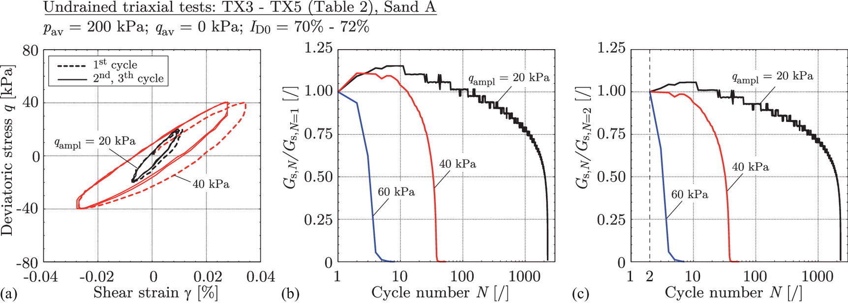
Fig. 9 shows demonstrative results of the undrained triaxial test with different definitions of the stiffness index. Fig. 9(a) shows the first three cycles of the tests with qampl = 20 and 40 kPa. The first cycle (dashed curve) indicates a visibly larger shear strain. The second and third cycles (solid line) exhibit a very similar hysteresis loop. In Fig. 9(b), the normalized secant shear modulus with Gs,N = 1 is shown. The secant shear moduli in the test with qampl = 20 and 40 kPa increase at the beginning of the test and then decrease during cyclic loading. The maximum growth at qampl = 20 is more than 15%, and that at qampl = 40 kPa exceeds 10%. This behavior agrees with the simple shear test results reported in Vucetic et al. (2021) and Vucetic and Mortezaie (2015). Fig. 9(c) presents the normalized modulus using Gs,N=2. Here, the curves start at N = 2, and the value of the first cycle is not considered. The development of the degradation curves Gs,N/Gs,N=2 follows a similar trend to that of the Gs,N/Gs,N=1 curves. However, for qampl = 40 kPa, the degradation curve does not show an increase at the beginning of the test. For qampl = 20 kPa, the growth in the secant shear modulus at the beginning is significantly smaller (5% versus 15%).
To demonstrate the influence of the irregular cycle, the triaxial test with qampl = 40 kPa (TX4) was repeated with an additional precycle. In this repeated test, the influence of the first cycle was eliminated during the precycle. The precycle was applied under drained conditions and exhibited the same amplitude. After the precycle, the density condition of the test changed only minimally. The loading scheme of the two tests is presented in Fig. 10(a). At the start of the tests (undrained conditions), both tests indicate the same stress conditions and similar densities. The development of the secant shear modulus and stiffness index fundamentally differ [Figs. 10(b and c)]. In the test with the precycle, the degradation curve does not show an increase at the beginning of the test. In other words, the increase in the degradation curves in the test without the precycle generates due to the atypically lower modulus GN=1 of the irregular cycle. The concept of the precycle to eliminate the effect of the irregular first cycle of undrained tests has been used in several studies (Wichtmann 2016; Wichtmann et al. 2010).

To quantify the cyclic degradation in the stiffness and the development of the secant shear modulus, the stiffness indexes δN (calculated with Gs,N = 1) dependent on the number of cycles are evaluated via simple shear tests (Tests SS9–SS24, Table 3). In the tests under constant-volume conditions [Figs. 11(a and c)], the stiffness index rapidly decreases to zero immediately after the specimen attains liquefaction. With small amplitudes, δN increases at the beginning of the test and reaches a peak (e.g., 1.11–1.15 for τampl = 5 and 7.5 kPa). Under a constant normal stress, the specimen is compacted under cyclic loading. The density continuously increases during the test. In comparison to the behavior under constant-volume conditions, the specimen under constant normal stress in drained condition shows a completely different trend. The stiffness under constant normal stress conditions significantly increases [Figs. 11(b and d)]. In most of the tests, δN grows in the first 100 cycles and remains relatively constant at a high level under further loading. For similar amplitudes, the tests with looser sand indicate a larger increase in the stiffness index.

Influence of the Stress Level
The stress level has a large influence on the stiffness of the soil. In this study, the dependency of the secant shear modulus on the stress level is investigated by means of a series of drained simple shear tests under strain-controlled cyclic loading. All tests presented in the previous sections are performed with stress-controlled cycles. In these tests, the shear strain amplitude changes continuously during cyclic loading. Therefore, to quantify the influence of the stress level, a series of strain-controlled simple shear tests with the same shear strain amplitude of γampl = 0.03% and at different consolidation stresses in the range of σv = 25‒300 kPa were carried out. Fig. 12 shows the evolution of the secant shear modulus with the number of cycles [Fig. 12(a)] and the stiffness index [Fig. 12(b)]. Under cyclic loading in drained conditions, the specimens become denser and stiffer. The secant shear modulus increases during the loading process. The stiffness index expresses the percentage growth of the secant shear modulus compared with the modulus at the beginning of the test (first cycle). It can be observed that the evolution of the stiffness index is greater in the test with lower stress levels. In the test with σv = 25 kPa, the secant shear modulus doubles after 1,000 cycles, while at σv = 300 kPa, the increase is 25%. The significant change is observed primarily in the first 100 cycles.

To quantify the effect of the stress level on the stiffness, the secant shear modulus measured in the 1st, 10th, and 1,000th cycles is utilized. The mean stress levels in the simple shear test cannot be directly evaluated due to the unknown horizontal stress. Therefore, the mean confining stress is assumed to be p = σv(1 + 2K0)/3 according to Silver and Seed (1971) with the coefficient K0 = 1–sin(φc). The parameter φc is the critical friction angle (Table 1). The results in Fig. 13 show that the secant shear modulus increases disproportionately with the mean confining stress. The pressure dependence of Gs can be described here with the exponential relationship Gs ∼ pn. Fitting to the test results gives an exponent of n = 0.78 for the modulus in the first cycle and n = 0.58 for the 1,000th cycle. The exponent n for describing Gs depends on the shear strain amplitude. For the same sand, an exponent of n = 0.52 is evaluated for Gmax based on the resonant column test results (Le 2015). According to Hardin and Black (1966) and Wichtmann and Triantafyllidis (2009), the average value for the exponent to describe Gmax is n = 0.5.

Isotropic and Anisotropic Loading Conditions
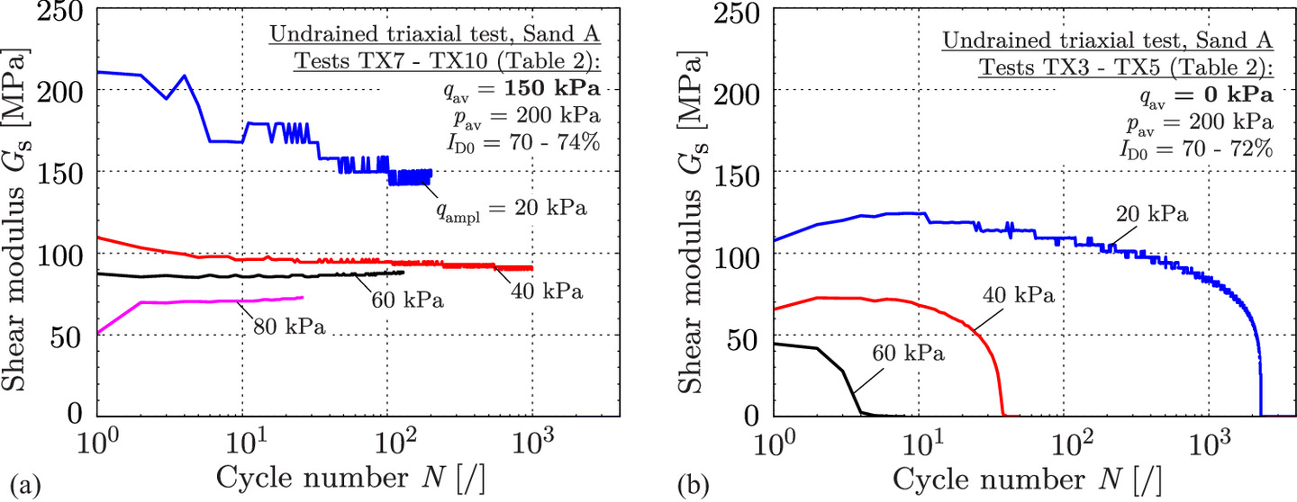
The influence of anisotropy in the loading condition can be investigated using triaxial tests. The development of the secant shear modulus in undrained triaxial tests under anisotropic and isotropic consolidation is presented in Fig. 14. All tests were conducted with the same mean confining stress pav = 200 kPa and similar densities. The amplitude qampl was adjusted from 20 to 80 kPa. Under undrained conditions, the test with qampl = 80 kPa liquefies within two cycles and is not presented in Fig. 14(b). All anisotropic tests involve 1,000 cycles [Fig. 14(a)]. However, due to the small range of the local displacement transducer and the large deformation of the specimens, the secant shear modulus here cannot be evaluated over the whole test. The tests show cyclic mobility under anisotropic conditions, and the cycle indicated a butterfly shape, while under isotropic conditions, the specimens experience liquefaction. The results show that the modulus in the anisotropic tests approaches a constant value, while the modulus is zero upon liquefaction under isotropic conditions.
Conclusions
An extensive laboratory program comprising several series of tests is carried out on medium and coarse sands using cyclic triaxial and simple shear devices. The drained and undrained tests in the study show, as expected, that the shape of the hysteresis loop depends on the loading and drainage conditions and can attain different forms. By the wide open stress‒strain loops, the secant shear moduli evaluated from the reloading and unloading branches can strongly differ. During cyclic loading, after a certain number of cycles, the difference between the reloading and unloading shear moduli decreases, and the cyclic loops close. It is well known that under drained and undrained conditions, soil stiffness develops in fundamentally different ways. During drained tests, the specimen becomes denser and stiffer, while during undrained tests, the specimen softens due to the development of excess pore-water pressure. This behavior can be confirmed by the secant shear modulus. At the beginning of the tests, the specimens under drained and undrained conditions exhibit a similar secant shear modulus. In the drained tests, the secant shear modulus increases with an increasing number of cycles. Under undrained conditions, the secant shear modulus decreases. The stiffness of the material is lost due to liquefaction, and the secant shear modulus is close to zero. Anisotropy has a significant influence on the undrained tests. Under anisotropic consolidation, the specimen reaches the state of cyclic mobility. In this state, although the accumulated shear strain increases continuously, the secant shear modulus tends to approach a constant value.
Appendix. Evaluation of the Secant Shear Modulus in the Triaxial Test
As mentioned previously, the secant shear modulus can be evaluated via two different methods [Eqs. (3) and (4)]. In most standard triaxial devices, measurement of the volumetric change of the specimen is possible. The radial strain ɛ3 can be estimated from the value of the volumetric strain ɛv. In some advanced devices, the radial strain ɛ3 can be directly measured using specific local displacement transducers (Wichtmann 2016; Goto et al. 1991). As such, the first method with Eq. (3) for secant shear modulus evaluation can be used. However, in certain situations (e.g., dry or unsaturated specimens in standard devices without local transducers), measurement of the radial strain is not obtainable. In this case, the second method with an assumption of Poisson's ratio ν by determination of the secant shear modulus from Young's modulus can be used [Eq. (4)]. In the undrained test, Poisson's ratio is ν = 0.5, and in the drained test, ν ranges from 0.20 to 0.40 (Wichtmann and Triantafyllidis 2009). To demonstrate the difference between these two methods, the secant shear modulus is evaluated through drained and undrained tests (Fig. 15).

In the undrained test, the two methods deliver the same results [Fig. 15(a)]. Under undrained conditions, the volume of the specimen remains constant, Poisson's ratio is ν = 0.5. In the drained test, Poisson's ratio is unknown. Estimation of Poisson's ratio leads to different results with Eq. (4). The area in gray in Fig. 15(b) represents the values of the secant shear modulus when we adjust Poisson's ratio from 0.25 to 0.35. For ν = 0.3, the results of this method suitably agree with those of the other method. For demonstration, the evaluation of the secant shear modulus for the fifth cycle of the Drained test TX1 (Table 2) according to Eqs. (3) and (4) is presented in Fig. 16.

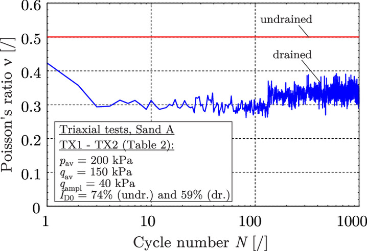
From the results of these triaxial tests, Poisson's ratio can be evaluated as ν = E/2Gs − 1. Therefore, Young's modulus can be calculated with the deviatoric stress and the axial strain [Eq. (4)], while the secant shear modulus can be evaluated with Eq. (3). Fig. 17 shows the development of Poisson's ratio with the number of cycles. In the undrained test, the ratio remained constant at 0.5. In the drained test, ν ranged from 0.27 to 0.38 (except for the first value). The estimation with ν = 0.3 for these tests [results presented in Fig. (15)] is reasonable up to 130 load cycles.
Data Availability Statement
Some or all data, models, or codes that support the findings of this study are available from the corresponding author upon reasonable request. They include the test results listed in Tables 2–4.
References
ASTM. 2003. Standard test methods for the determination of the modulus and damping properties of soils using the cyclic triaxial apparatus. ASTM D3999-1991 (Reapproved 2003). West Conshohocken, PA: ASTM.
ASTM. 2019. Standard test method for consolidated undrained direct simple shear test under constant volume with load controll or displacement controll. ASTM D8296-19. West Conshohocken, PA: ASTM.
Bai, L. 2010. “Preloading effects on dynamics sand propeties.” Ph.D. thesis, Publication of the Soil Mechanics and Geotechnical Engineering Div., Technische Universität Berlin.
DIN (Deutsche Institut für Normung e.V.). 2022. Soil, investigation and testing-Determination of density of non cohesive soils for maximum and minimum compactness. DIN 18126:2022-10. Berlin: Beuth Verlag.
Doroudian, M., and M. Vucetic. 1995. “A direct simple shear device for measuring small-strain behavior.” Geotech. Test. J. 18 (1): 69–85. https://doi.org/10.1520/GTJ10123J.
Glasenapp, R. 2016. “Behavior of sand under cyclic irregular loading.” Ph.D. thesis. [In German.] Ph.D. thesis, Soil Mechanics and Geotechnical Engineering Div., Technische Universität Berlin. https://doi.org/10.14279/depositonce-5402.
Goto, S., F. Tatsuoka, S. Shiubuya, Y. S. Kim, and T. Sato. 1991. “A simple gauge for local small strain measurements in the laboratory.” Soils Found. 31 (1): 169–180. https://doi.org/10.3208/sandf1972.31.169.
Hardin, B. O., and W. L. Black. 1966. “Sand stiffness under various triaxial stresses.” J. Soil Mech. Found. Div. 92 (SM2): 27–42. https://doi.org/10.1061/JSFEAQ.0000865.
Hardin, B. O., and V. P. Drnevich. 1972. “Shear modulus and damping in soils: Design equation and curves.” J. Soil Mech. Found. Div. 89 (7): 667–692. https://doi.org/10.1061/JSFEAQ.0001760.
Idriss, I. M., R. Dobry, and R. D. Singh. 1978. “Nonlinear behavior of soft clays during cyclic loading.” J. Geotech. Eng. Div. 104 (12): 1427–1447. https://doi.org/10.1061/AJGEB6.0000727.
Kukusho, T. 1980. “Cyclic triaxial test of dynamic soil properties for wide strain range.” Soils Found. 20 (2): 45–60. https://doi.org/10.3208/sandf1972.20.2_45.
Le, V. H. 2015. “Behavior of sand under cyclic loading with polarization changes in simple shear test.” [In German.] Ph.D. thesis. Publications of the Soil Mechanics and Geotechnical Engineering Div., Technische Universität Berlin. https://doi.org/10.14279/depositonce-4896.
Le, V. H., and F. Rackwitz. 2020. “A new cyclic simple shear test procedure with multidirectional loading.” Geotech. Test. J. 43 (1): 275–286. https://doi.org/10.1520/GTJ20180074.
Mortezaie, A. R., and M. Vucetic. 2012. “Small-strain cyclic testing with standard NGI simple shear device.” Geotech. Test. J. 35 (6): 935–948. https://doi.org/10.1520/GTJ20120007.
Niemunis, A., T. Wichtmann, and Th. Triantafyllidis. 2005. “A high-cycle accumulation model for sand.” Comput. Geotech. 32 (4): 245–263. https://doi.org/10.1016/j.compgeo.2005.03.002.
Park, T. K., and M. L. Silver. 1975. “Dynamic triaxial and simple shear behavior of sand.” J. Geotech. Eng. Div. 101 (6): 513–528. https://doi.org/10.1061/AJGEB6.0000170.
Seed, H. B., R. T. Wong, I. M. Idriss, and K. Tokimatsu. 1986. “Moduli and damping factors for danamic analyses of cohesionless soils.” J. Geotech. Eng. 112 (11): 1016–1032. https://doi.org/10.1061/(ASCE)0733-9410(1986)112:11(1016).
Silver, M. L., and H. B. Seed. 1969. The behavior of sands under seismic loading conditions. Rep. No. EERC 69-16. Berkeley, CA: Univ. of California.
Silver, M. L., and H. B. Seed. 1971. “Deformation characteristics of sand under cyclic loading.” J. Soil Mech. Found. Div. 97 (8): 1081–1098.
Skempton, A. W. 1954. “The pore-pressure coefficients A and B.” Geotechnique 4 (4): 143–147. https://doi.org/10.1680/geot.1954.4.4.143.
Song, B., K. Yasuhara, and S. Murakami. 2004. “Direct simple shear testing for post-cyclic degradation in stiffness of nonplastic silt.” Geotech. Test. J. 27 (6): 607–613. https://doi.org/10.1520/GTJ11194.
Vucetic, M. 1988. “Normalized behavior of offshore clay under uniform cyclic loading.” Can. Geotech. J. 25 (1): 33–41. https://doi.org/10.1139/t88-004.
Vucetic, M. 1994. “Cyclic threshold shear strains in soils.” J. Geotech. Eng. 120 (12): 2208–2228. https://doi.org/10.1061/(ASCE)0733-9410(1994)120:12(2208).
Vucetic, M., and R. Dobry. 1991. “Effect of soil plasticity on cyclic response.” J. Geotech. Eng. 117 (1): 89–107. https://doi.org/10.1061/(ASCE)0733-9410(1991)117:1(89).
Vucetic, M., and A. Mortezaie. 2015. “Cyclic secant shear modulus versus pore water pressure in sands at small cyclic strains.” Soil Dyn. Earthquake Eng. 70: 60–72. https://doi.org/10.1016/j.soildyn.2014.12.001.
Vucetic, M., and K. Tabata. 2003. “Influence of soil type on the effect of strain rate on small-strain cyclic shear modulus.” Soils Found. 43 (5): 161–173. https://doi.org/10.3208/sandf.43.5_161.
Vucetic, M., H. Thangavel, and A. Mortezaie. 2021. “Cyclic secant shear modulus and pore water pressure change in sand at small cyclic strains.” J. Geotech. Geoenviron. Eng. 147 (5): 04021018. https://doi.org/10.1061/(ASCE)GT.1943-5606.0002490.
Wichtmann, T. 2005. “Explicit accumulation model for non-cohesive soil under cyclic loading.” Ph.D. thesis. Publications of the Institute of Soil Mechanics and Foundation Engineering, Ruhr-Universität Bochum.
Wichtmann, T. 2016. “Soil behaviour under cyclic loading–Experimental observations, constitutive description and applications.” Habilitaion thesis. Publications of the Institute for Soil Mechanics and Rock Mechanics, Karlsruhe Institute of Technology (KIT).
Wichtmann, T., A. Niemunis, B. Rojas, and T. Triantafyllidis. 2010. “Stress- and strain-controlled undrained cyclic triaxial tests on a fine sand for a high-cycle accumulation model.” In Proc., Fifth Int. Conf. on Recent Advances in Geotechnical Earthquake Engineering and Soil Dynamics. Rolla, MO: Missouri University of Science and Technology.
Wichtmann, T., and T. Triantafyllidis. 2009. “On the influence of the grain size distribution curve of quartz sand on the small strain shear modulus Gmax.” J. Geotech. Geoenviron. Eng. 135 (10): 1404–1418. https://doi.org/10.1061/(ASCE)GT.1943-5606.0000096.
Wichtmann, T., and T. Triantafyllidis. 2013. “Effect of uniformity coeficient on G/Gmax and damping ratio of uniform to well graded quartz sands.” J. Geotech. Geoenviron. Eng. 139 (1): 59–72. https://doi.org/10.1061/(ASCE)GT.1943-5606.0000735.
Information & Authors
Information
Published In

International Journal of Geomechanics
Volume 24 • Issue 7 • July 2024
Copyright
This work is made available under the terms of the Creative Commons Attribution 4.0 International license, https://creativecommons.org/licenses/by/4.0/.
History
Received: Jul 2, 2023
Accepted: Jan 13, 2024
Published online: Apr 26, 2024
Published in print: Jul 1, 2024
Discussion open until: Sep 26, 2024
Authors
Metrics & Citations
Metrics
Citations
Download citation
If you have the appropriate software installed, you can download article citation data to the citation manager of your choice. Simply select your manager software from the list below and click Download.