Leakage Detection in Water Distribution Systems Based on Logarithmic Spectrogram CNN for Continuous Monitoring
Publication: Journal of Water Resources Planning and Management
Volume 150, Issue 6
Abstract
In the context of the Internet of Things, there is a growing demand for real-time monitoring of water distribution systems (WDS). Among the various leak detection methods, acoustic leak detection is considered to be a suitable method. However, existing methods are not very effective in environments with high daytime ambient noise. To address this issue, this paper conducted on-site data collection experiments and designed a monitoring system that combines traditional nighttime monitoring with daytime monitoring, combining water company pipeline inspections and repair work. A large number of daytime audio samples were collected. In this paper, the logarithmic spectrogram (log spectrogram) was used to represent the features of the leak signal. By comparing the features of the signal during day and night, noisy and quiet environments, and leak and normal signals, we identified the interfering frames that required noise reduction, and applied frame-level noise reduction processing to the signal. Based on this, a log PS-ResNet18 model was developed to identify leaks, and its performance was compared with other classification models [including traditional nighttime detection methods, random forests, XGBoost, and convolutional neural network (CNN)]. The results showed that the log PS-ResNet18 model had the best performance, with an all-day accuracy rate of 99.4% and a daytime accuracy rate of 99.3%. In addition, by conducting ablation experiments to explore the role and contribution of the log PS-ResNet18 and noise reduction methods in the model, the results showed that the log spectrogram and noise reduction methods increased the all-day accuracy rate by 18.8% and 23.2%, respectively, and by 24.7% when used together. In another practical application, the log PS-ResNet18 model achieved an all-day detection accuracy rate of 99.6%. This study demonstrated the applicability of the log spectrogram and CNN combination in daytime leak detection, overcoming research limitations in the field.
Practical Applications
This research presents the log PS-ResNet18 framework, which combines deep learning models and denoised logarithmic spectrograms to improve leak detection in water supply pipelines under daytime environmental noise. The research focuses on field data collection and analysis of cast iron pipes with different diameters in Hangzhou (HZ). The model was tested on cast iron pipes in Lishui (LS) and proved to be effective. The proposed method is highly versatile and can be applied to different regions and pipe materials after sufficient sample collection and model training validation. The research recommends a comprehensive leak monitoring solution that involves initial intelligent detection using front-end noise meters and secondary identification of suspicious audio signals using the log PS-ResNet18 model in the cloud. This enables water utility operators to respond quickly to pipeline leaks, leading to more efficient water resource conservation and improved water supply service quality.
Introduction
Water distribution systems (WDS) are a critical component of water supply systems, and their healthy operation plays an important role in ensuring the stable delivery of water resources. Statistics show that water loss caused by leaks or pipe breaks in WDS accounts for about 10% to 30% of urban water use (Kang et al. 2017). Due to the invisibility of hidden pipe leaks, the water loss caused by them is more severe. Hidden leaks occur more frequently compared to pipe bursts. Therefore, identifying leaks in WDS is crucial for ensuring the stable delivery of water resources (Mounce et al. 2010; Wang et al. 2022; Xin and Wu 2020). It is crucial to detect and repair hidden leaks as early as possible to prevent continuous water loss and worsening of the leaks. Among the various methods for leak detection in WDS, the acoustic emission method is nondestructive, accurate, and efficient (Diao et al. 2020; Fantozzi and Fontana 2001; Fuchs and Riehle 1991), making it suitable for real-time monitoring (Fan et al. 2022). The leak sound wave is caused by the interaction between the water at the leak point and the pipe wall; therefore, it is a random signal with short-term nonstationary and long-term stationary components. Its propagation characteristics in the pipeline are mainly reflected in: (1) the lower the elastic modulus of the pipe material, the lower the frequency of the leak signal, (2) the higher the pressure inside the pipe, the stronger the leak sound signal and the more high-frequency components, (3) the energy attenuation occurs during sound wave propagation, with high frequencies attenuating faster than low frequencies, and the energy of the high-frequency part being more concentrated closer to the leak point, (4) the sound wave energy during a leak condition is higher than during normal conditions, increasing first and then decreasing with an increase in the leak hole size, while the sound wave energy during normal conditions increases with an increase in pipeline pressure, and (5) the frequency components of the leak sound signal produced during the initial stage of a leak are complex and unstable.
Currently, noise logger leak detection methods can be mainly divided into two categories: traditional pattern recognition methods and deep learning-based methods (Guo et al. 2021). Traditional pattern recognition methods use time-domain and frequency-domain features for identification. Lim (2014) detected leaks by using a predefined threshold based on the change of the crest factor (CF) with flow rate and pressure. Martini et al. (2015) developed a monitoring algorithm based on standard deviation, which also uses a predefined threshold for leak detection. Martini et al. (2018) developed a leak detection method using the autocorrelation function and selected the kurtosis of normalized autocorrelation as a feature. This method was validated in on-site tests with artificially generated leaks. Tariq et al. (2022) combined Martini’s monitoring algorithm based on standard deviation with machine learning models such as k-nearest neighbor, decision tree, random forest, and adaptive boosting (Adaboost) for leak and nonleak classification. However, traditional methods rely on prior knowledge and experience of the signal for feature selection, and their detection performance is often influenced by environmental noise and high-energy interference, which limits their applicability in practical scenarios (Xin and Wu 2020). In recent years, deep learning-based methods have received widespread attention in leak detection and achieved good results. Kang et al. (2017) proposed an adaptive design leakage detection system that combines one-dimensional convolutional neural networks (CNNs) and support vector machines (SVMs) for leak detection. Zhou et al. (2019) designed a new DNN-based model. Guo et al. (2021) proposed a time-frequency CNN model (TFCNN) and mixed the original nighttime signal with white Gaussian noise (WGN) during the data set construction phase to simulate different signal-to-noise ratio (SNR) conditions and test the effect of noise on the detection model. Although these models have achieved good results, most of the studies focus on nighttime audio data in the field or laboratory data, which does not meet the requirements for round-the-clock monitoring in the field. Moreover, the noise components in actual WDS are complex and not just simple white noise. Therefore, daytime leak detection has become an urgent practical problem that requires real-time monitoring experiments on actual WDS and solving the problem of high-energy noise interference (Fan et al. 2022).
Extracting more valuable feature information from signals is beneficial for leak detection. Time-frequency domain features express the changes of time-frequency content with time and often appear in the form of spectrograms, which represent three-dimensional information on a two-dimensional plane and can provide more valuable information for complex signals that are difficult to describe with time-domain or frequency-domain features. Therefore, in recent years, spectrograms have often been used as inputs for deep learning. Shukla and Piratla (2020) used scalogram images of acceleration signals to establish a deep learning model. Guo et al. (2021) proposed using linear spectrograms to characterize audio signal features. Cody et al. (2020) proposed a semisupervised method based on hydroacoustic spectrograms of underwater acoustic signals. However, this method may have limitations in noisy environments (Fan et al. 2022). Since the amplitude range of linear spectrogram or scalogram images is linear, the dynamic range is limited, resulting in less richness of details and colors in the images. Therefore, the above studies did not fully explore the time-frequency domain features of the signals. On the other hand, log spectrograms exhibit advantages in terms of dynamic range.
To address these issues, this study first designed a field data collection experiment, using noise loggers to monitor an actual water distribution system for 24 h a day to collect and obtain audio signals of the water distribution system under both normal and leak conditions. Secondly, log spectrograms were used to represent the audio signals, and a frame-level denoising method was applied to remove high-energy background noise from the signals as much as possible. The denoised log spectrograms were used as inputs for the CNN deep learning model to perform daytime leak detection, and were compared with other classification models. Finally, the models were evaluated and analyzed separately for noisy daytime environments and quiet nighttime environments.
The contributions of this paper mainly include the following aspects:
1.
Designed and conducted a real-world noise logger data collection experiment for WDS, collecting a large number of samples in relatively noisy daytime environments to conduct daytime leak detection.
2.
The short time Fourier transform (STFT) method is employed to create log spectrograms to represent the time-frequency characteristics of the detection signals, and optimize the parameters to fully exploit the time-frequency domain features of the signals and improve the detection capability of the model.
3.
Proposed a method to identify and denoise high-energy background noise to reduce noise interference.
4.
Developed a deep learning model based on log spectrograms and achieved feasible daytime leak detection technology under real-world conditions of WDS.
Methodology
Spectrogram
Guo et al. (2021) showed through experiments that under low SNR conditions, linear spectrogram features are more stable than time-domain or frequency-domain features, which helps to improve the reliability of the model; time-domain or frequency-domain features are susceptible to noise interference, leading to poorer model performance. Linear spectrograms are images that display the amplitude distribution of signal frequency components in both time and frequency domains, and are commonly used to analyze the frequency distribution of continuous signals such as audio signals and seismic waves. Linear spectrograms can decompose signals into two parts: the time domain and frequency domain, which can be used to represent the distribution on the time axis and the frequency axis. In linear spectrograms, time is usually represented along the horizontal axis, frequency along the vertical axis, and the amplitude of signal frequency components is represented by color or brightness.
Similarly, log spectrograms are also images that represent the energy distribution of signals in both time and frequency domains, but with the amplitude values using logarithmic values (Dennis et al. 2010). In this paper, linear spectrograms and log spectrograms were established based on STFT, with the following basic steps: (1) the original signal is segmented into frames, and the duration of each frame is called the frame length. In order to ensure the smoothness of audio feature parameters, overlapping frames are usually used, and there is a staggered part between adjacent frames, which is called the frame shift; (2) the original signal is windowed: frame segmentation is equivalent to adding a rectangular window to the audio signal, which truncates the signal in the time domain and causes multiple side lobes at the edge, resulting in spectral leakage. In order to reduce spectral leakage, other forms of windowing operations are usually performed on the segmented signal, including Hamming window, Hanning window, etc.; (3) perform Fourier transform on each segmented signal after windowing to obtain the representation of each frame signal in the frequency domain. At this point, all frames are arranged in order to obtain a linear spectrogram; and (4) on this basis, perform logarithmic transformation on the squared amplitude of each frequency component at each moment, with the unit being decibel (dB). At this point, all frames are arranged in order to obtain a log spectrogram.
When STFT is used to generate spectrograms, time resolution can be adjusted by changing the window length, while frequency resolution can be adjusted by changing the fast Fourier transform (FFT) length. Specifically, shorter window lengths result in higher time resolution, which can better capture short-term changes in the signal, while longer FFT lengths for each frame result in higher frequency resolution, which can better distinguish different frequency components in the signal. Therefore, adjusting the window length and FFT length can balance time and frequency resolution to obtain the best spectrogram analysis results. For audio with a sampling frequency of 8 kHz, the length of each frame is usually set to 20–40 ms (i.e., the frame length). Meanwhile, the ratio of frame shift to frame length is often set to to fully utilize the time information of the signal and avoid information overlap between adjacent frames. The specific frame length and frame shift can be adjusted according to actual needs to obtain the optimal spectrogram analysis results. The FFT length is usually specified as a power of 2, such as (128–512). This allows for easy computation using the FFT algorithm and provides relatively high-frequency resolution.
Denoising of High-Energy Background Noise
One of the challenges in daytime leak detection is the interference of high-energy background noise in noisy environments (Adedeji et al. 2017; Chan et al. 2018; Fan et al. 2022). Low-frequency high-energy background noise is more common, with frequencies often concentrated in the low frequency range (0–300 Hz), which does not overlap with the frequency bands related to leakage caused by metal pipelines. To reduce the impact of low-frequency high-energy noise, methods such as low-pass filtering and preemphasis are commonly used (Bhangale and Mohanaprasad 2022). In urban environments, common sources of high-energy noise include industrial activity, traffic noise such as car horns and manhole cover rolling, and other noises such as construction and raindrops. Such noise has a high amplitude and nonconcentrated frequency characteristics in the frequency domain, and is a type of random high-energy background noise.
El-Abbasy et al. (2016) stated that background noise and leakage noise exhibit different frequency-domain distribution characteristics over time. Background noise, due to its strong randomness, typically has wide bandwidth and nonstationary characteristics, is clearly time-varying, and exhibits a divergent spectral distribution. Leakage noise, on the other hand, is a short-term nonstationary and long-term stationary random signal with clear time invariance and locality, and exhibits a concentrated spectral distribution. Based on these characteristics, (1) interference signals are identified, and the frequency-domain characteristics of each frame are analyzed. Frames with high-energy noise are identified by their high average and high standard deviation of spectral values (Fan et al. 2022; Martini et al. 2015). If the average and standard deviation of the spectral values of a frame exceed certain limits, the frame is considered to be an interference frame (see Case Study for details), and (2) denoising of the interference frames is performed by calculating and retaining only 1–2 local energy peaks in each frame. Under leak conditions, the retained energy peaks will reflect the characteristics of the leakage signal. Under normal conditions, even if there is high background noise, the retained wide frequency features can still be distinguished from the leakage signal features. In addition, since continuous high-energy low-frequency noise has similar time-frequency characteristics to leakage signals, processing of the corresponding low-frequency band is required to eliminate its influence on the peak retention method before peak retention operation. Generally, truncation of the low-frequency band or reassignment of values to the low-frequency band can achieve the desired effect.
ResNet Model and Evaluation Metrics
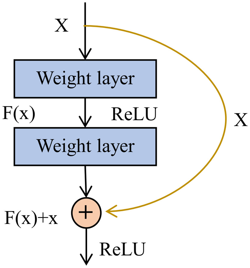
ResNet (Residual Network) is a type of CNN structure proposed by He et al. (2016) in 2015, aimed at solving the problem of vanishing gradients in deep neural networks. The core idea of ResNet is to introduce residual connections between certain layers in the network. These connections allow the network to skip some layers and directly transmit information from one layer to another. Residual connections effectively create a shortcut path in the network, making it easier to learn and reducing the likelihood of vanishing gradients.
As shown in Fig. 1, the structure of a ResNet block typically includes two or more convolutional layers, followed by a batch normalization layer and a nonlinear activation function, such as ReLU (Rectified Linear Unit). The output of the block is then added to the inputs through a residual connection, and the result is passed through another activation function. This structure is repeated multiple times throughout the network, with the number of blocks and the number of filters in each block varying depending on the specific ResNet architecture used.
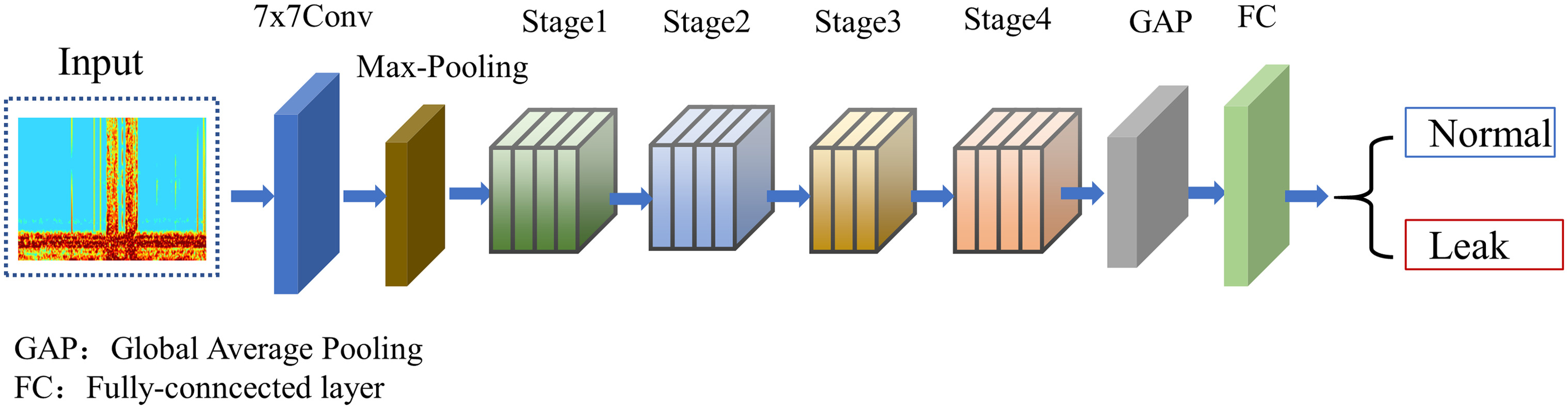
As shown in Fig. 2, ResNet18 (Odusami et al. 2021) consists of 18 layers, including a convolutional layer, four residual blocks, a global average pooling layer, and a fully connected layer. Because the ResNet18 model is relatively small, it is often used for computer vision tasks such as image classification and object detection when computing resources are limited. It has good performance on many computer vision tasks and relatively fast training speed, making it suitable for edge computing and deployment.
For performance evaluation of binary classification models, a confusion matrix can be used to count true negatives (TNs), false negatives (FNs), true positives (TPs), and false positives (FPs), and calculate metrics such as accuracy, recall, and precision. Here, true positive (TP) indicates that a leak event is correctly detected, false positive (FP) indicates that a normal event is incorrectly identified as a leak event, true negative (TN) indicates that a normal event is correctly identified, and false negative (FN) indicates that a leak event is not detected. Accuracy represents the proportion of correctly classified samples, recall represents the proportion of actual leaks that are correctly identified among all actual leaks, and precision represents the proportion of correctly classified positive samples (i.e., leak event) among all samples classified as positive. In addition, F1-score is also a commonly used binary classification metric, which combines recall and precision, with a larger value indicating better model performance. An F1-score greater than 0.9 usually indicates practical value of the model.
Comparison of Classification Models
To more accurately evaluate the performance of the proposed method in this article, it will be compared with other classification methods. In traditional pattern recognition methods, a commonly used approach is to classify signals using predefined thresholds, while machine learning methods are more complex but typically achieve better performance. Martini et al. (2015) proposed a traditional detection algorithm based on the standard deviation (STD) of the amplitude of the original signal, which calculates the standard deviation of the amplitude of the original signal as the monitoring index (MI), and obtained the monitoring index efficiency (MIE) by comparing it with the preset MI (). Each type of pipeline has a different MIE, for further details see Tariq et al. (2022). When the MIE value exceeds a certain threshold, a leakage alarm is triggered, thus achieving automatic leakage detection. This method has been applied by Tariq et al. (2022) and has achieved high accuracy in nighttime leak detection, demonstrating its applicability in traditional signal processing.
Supervised machine learning models typically use time-domain and frequency-domain features as inputs to construct classification models. Random forest (RF) and extreme gradient boosting (XGBoost) are tree-based ensemble models that combine multiple decision trees to improve classification performance, and have strong classification capabilities. Several studies (Guo et al. 2022, 2021; Tariq et al. 2022) have demonstrated their applicability in related fields. Based on previous research, commonly used time-domain features for machine learning include root mean square, standard deviation, and crest factor (CF), while commonly used frequency-domain features include the average decibel of power spectral density and zero-crossing rate.
Guo et al. (2021) proposed a time-frequency convolutional neural network (TFCNN) that recognizes leaks by using a CNN model to analyze three linear spectrograms with different resolutions. The model inputs include high time resolution, high-frequency resolution, and harmonically resolved time-frequency spectrograms. TFCNN has three parallel CNN layers, each corresponding to one of the linear spectrograms, followed by a max pooling layer and a batch normalization layer. The merge layer connects the output tensors of the previous layer. Finally, the output tensor is connected to several fully connected layers and an exit layer. Guo et al. (2021) reported that this model achieved an average accuracy of 98% on raw data and white Gaussian noise (WGN) mixed detection signals collected at night, even under different SNR conditions. The average detection accuracy reached 90% even at a SNR of .
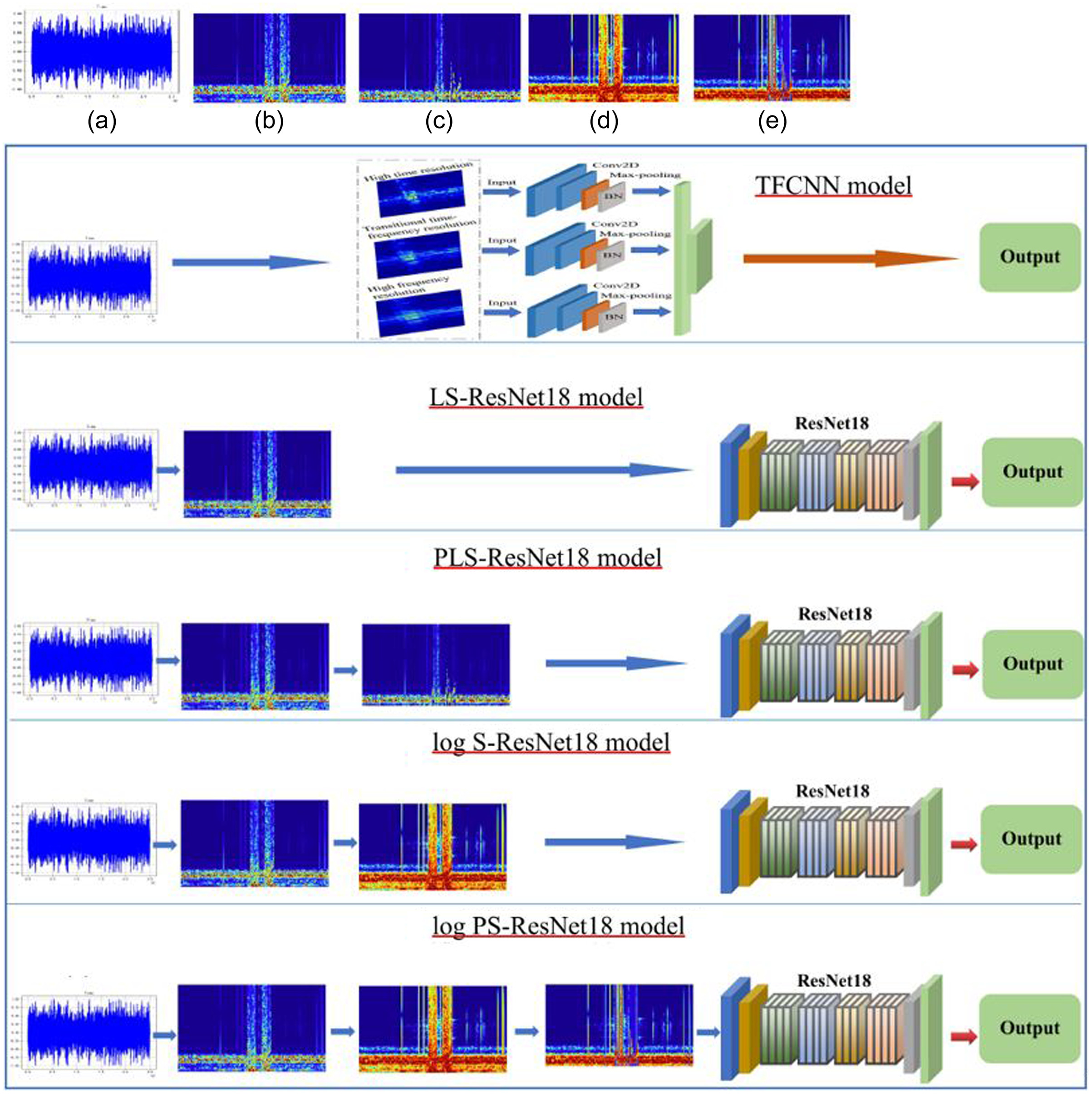
The improvement proposed in this article is to use log spectrograms as features and adopt peak retention denoising technology. In order to clarify the effects of these two improvement methods, an ablation experiment was designed, and three classification models were added: the Linear Spectrogram ResNet18 model (LS-ResNet18 model), the Peak Retention Linear Spectrogram ResNet18 model (PLS-ResNet18 model), and the Log Spectrogram ResNet18 model (log S-ResNet18 model). These models were compared with the Log Peak Retention Spectrogram ResNet18 model (log PS-ResNet18 model) proposed in this article. All of these models used the ResNet18 CNN model, but with different inputs. The LS-ResNet18 model used linear spectrograms as inputs, the PLS-ResNet18 model used peak retention denoised linear spectrograms as inputs, the log S-ResNet18 model used log spectrograms as inputs, and the log PS-ResNet18 model used peak retention denoised log spectrograms as inputs. Fig. 3 shows the structures of the five different CNN models.
Case Study
Experimental Setup
The experimental equipment consisted of noise loggers and a pipeline leakage monitoring cloud platform developed by our collaborating partners. The noise logger adopts a high-sensitivity piezoelectric sensor and is installed by magnetic attachment to metal pipe sections or valves. The sampling frequency is 8 kHz, and the sampling precision is 16 bits. Equipped with NB remote transmission and Lora short-range inspection antennas, it had functions of night and day monitoring and synchronous detection of multiple measuring points. The cloud platform collected and stored the original data (audio and parameters) in real-time, and had functions such as audio playback and routine detection. The experiment revolves around the water company’s actual leak detection and maintenance work. When the leak detection personnel identify a pipeline leakage and there is no urgency for immediate repair, and there are nearby inspection wells, the research team members are notified to arrange the placement of noise loggers and collect data. Typically, 5–6 noise loggers are deployed in the inspection wells around the actual leakage point, generally within a distance of 200 meters. Continuous data was collected for 5–7 days before and after repairs (1–2 days before repairs and 4–5 days after repairs), with audio data collected/uploaded every hour to ensure the collection of leakage/normal sample data of various pipe diameters and all-weather conditions. At the same time, the traditional nighttime monitoring method was retained, with audio signal amplitude STD calculated every 100 s from midnight to 4 a.m., with 36 groups collected per hour and the smallest 10 groups used to calculate the average value, saved and uploaded for MI threshold detection method.
The experiment lasted for one year from November 2021 to November 2022, and the water supply network is a circular layout, supplied by three water plants. Within residential areas and units, a secondary water supply system is implemented. The water pressure in the municipal network generally ranges from 0.25 MPa to 0.3 MPa. A total of 12,316 audio samples were collected and organized from more than 10 different actual pipeline sections in HZ city, of which 3,435 samples were labeled as leaks and 8,881 samples were labeled as normal. The pipeline materials include galvanized steel pipes and ductile iron pipes, with pipe sizes ranging from DN100 to DN400 (diameter 100 to 400 mm). The entire data set was randomly divided into an 80% training data set and a 20% testing data set. The audio samples were single-channel audio with a duration of 2.5 s. The division of daytime and nighttime periods was the same as that of traditional nighttime monitoring, with 10,298 daytime audio samples and 2,018 nighttime audio samples. The data calculations of this experiment were implemented using Python programming.
Plotting Log Spectrograms
In STFT, the FFT length, frame length, frame shift, and window function are important parameters that affect the size and time-frequency resolution of the spectrogram. In previous studies, the frame length was set equal to the FFT length, which made it difficult to balance the time and frequency resolution and led to poor detection performance. Although multiple resolution images can be used as inputs, this increases the complexity of the model. In this paper, the sampling frequency remains constant at 8,192 Hz, we use an FFT length of (512) to obtain higher frequency resolution. At the same time, the frame length of 25 ms (205) and frame shift of 10 ms (82) can achieve higher time resolution and ensure that there is enough data for the FFT calculation. The Hann window is a commonly used window function known for providing good frequency resolution and side-lobe suppression capabilities in spectral analysis. In this paper, the Hann window is used to estimate the spectrum. After these processing steps, we can obtain the raw data for plotting linear spectrograms. By squaring the data and taking the logarithm, we obtain the log spectrograms.
When plotting the spectrogram, the color mapping and value range are two key parameters that can significantly affect the visual performance of the spectrogram. The color mapping converts numerical values into colors, with a dark blue set as the minimum value and light blue, light green, yellow, orange, red, and dark red representing increasing values. The amplitude range of the linear spectrogram is set to [0, 12] using a linear scale, while the color of the log spectrogram represents the energy in decibel (dB) units using a logarithmic scale, with a value range of [–100,–20]. Setting a reasonable value range can reduce the impact of outliers on the spectrogram and improve the detection performance.
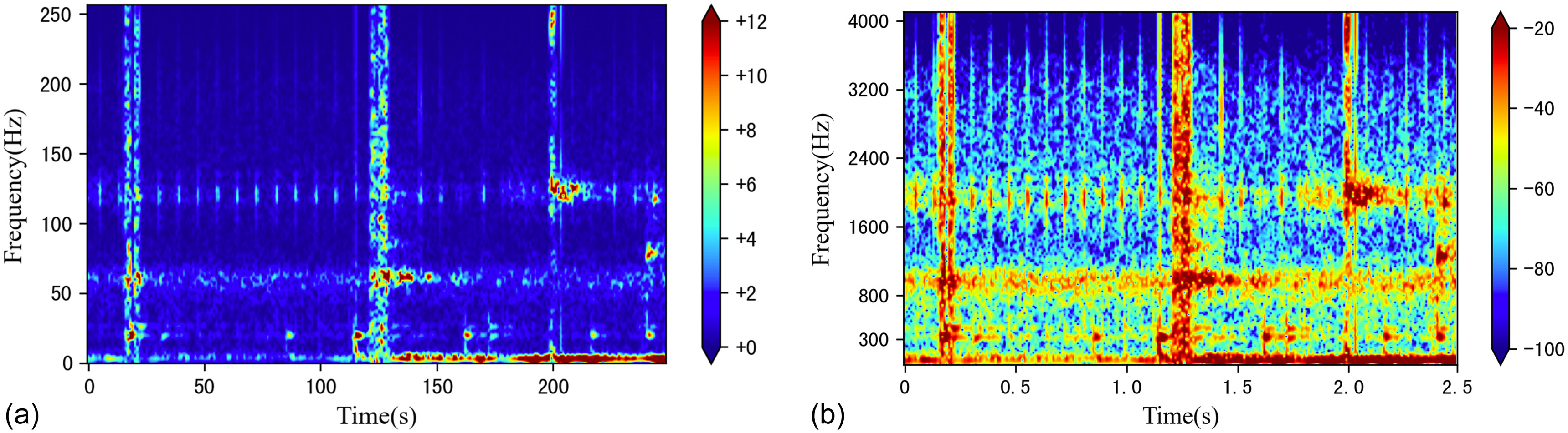
Compared to linear spectrograms, log spectrograms have a wider dynamic range, which can more prominently display differences and energy distributions between signals and are more suitable for comparing the strength and energy distribution of different signals. Therefore, using log spectrograms to characterize the time-frequency features of audio signals is more appropriate. Fig. 4 shows the linear and log spectrograms of the same audio, demonstrating the advantages of the log spectrogram.
Extracting Features as Model Inputs
As shown in Fig. 5, the log peak retention spectrogram (log P-Spectrogram) is used to extract signal features. First, the original signal is divided into frames and windowed, and then FFT is performed to obtain a linear spectrogram. Next, data within the frequency range of 0–300 Hz is removed, and interference frames are identified for each frame of the signal. For frames that are identified as interference frames, peak retention denoising technology is used to obtain the peak retention linear spectrogram (PL-Spectrogram). Finally, the matrix is mathematically transformed by taking the logarithm, resulting in the matrix for the log P-Spectrogram.
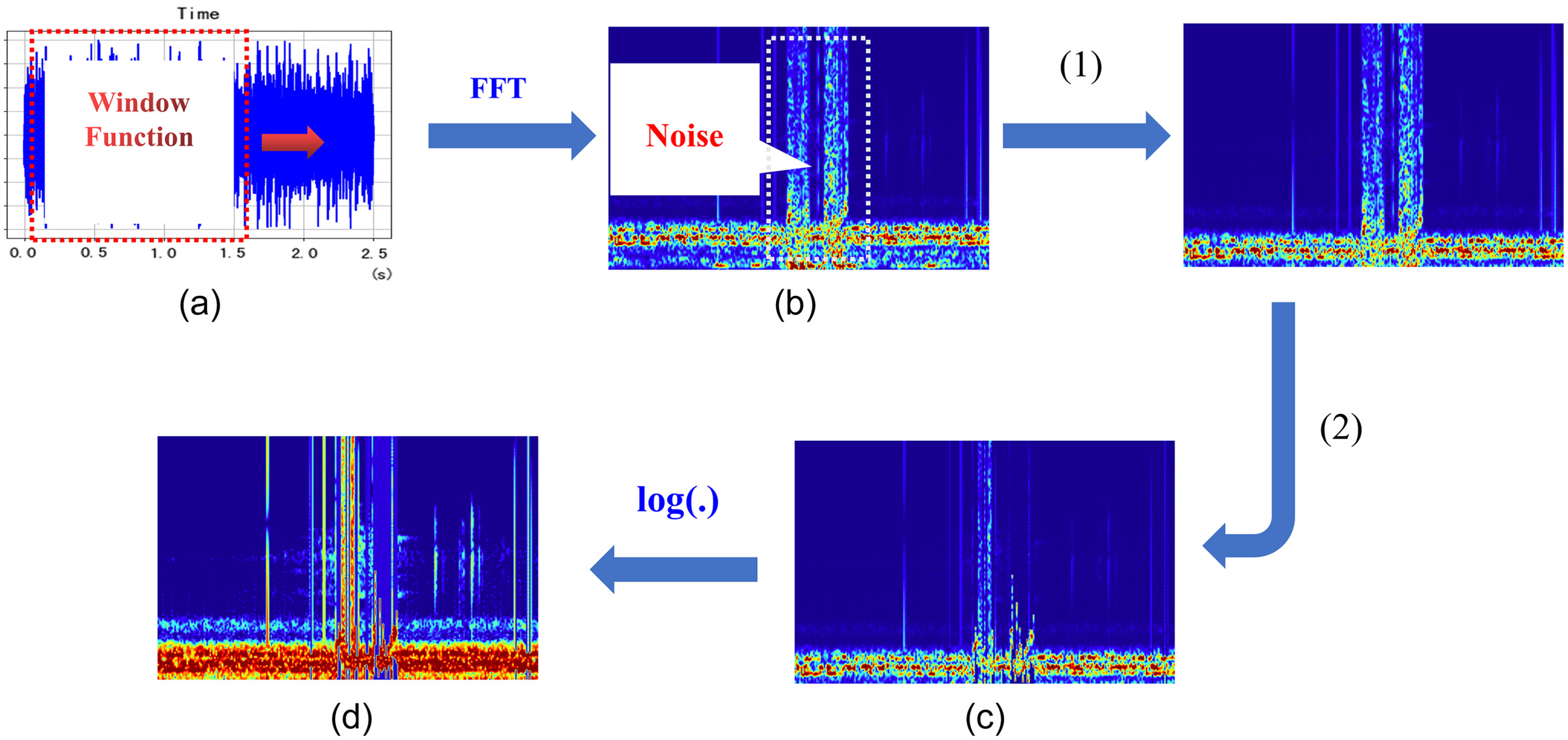
Fig. 6(a) shows the log spectrogram of a leak sample before denoising. The -axis represents time (s), and the -axis represents frequency (Hz). The stable leak signal appears in specific frequency bands based on the pipe material, diameter, and distance from the leak point. The leak signals generated in metal pipes have frequencies higher than 300 Hz. For metal pipes, the leak frequency is higher than 300 Hz. The noise mainly consists of high background noise in the low-frequency band and random high background noise. In this study, to address the high background noise in the low-frequency band, the low-frequency band of 0–300 Hz is removed to extract the relevant frequency bands caused by leaks. The main reason for doing this is to avoid the influence of low-frequency signals during frame denoising.
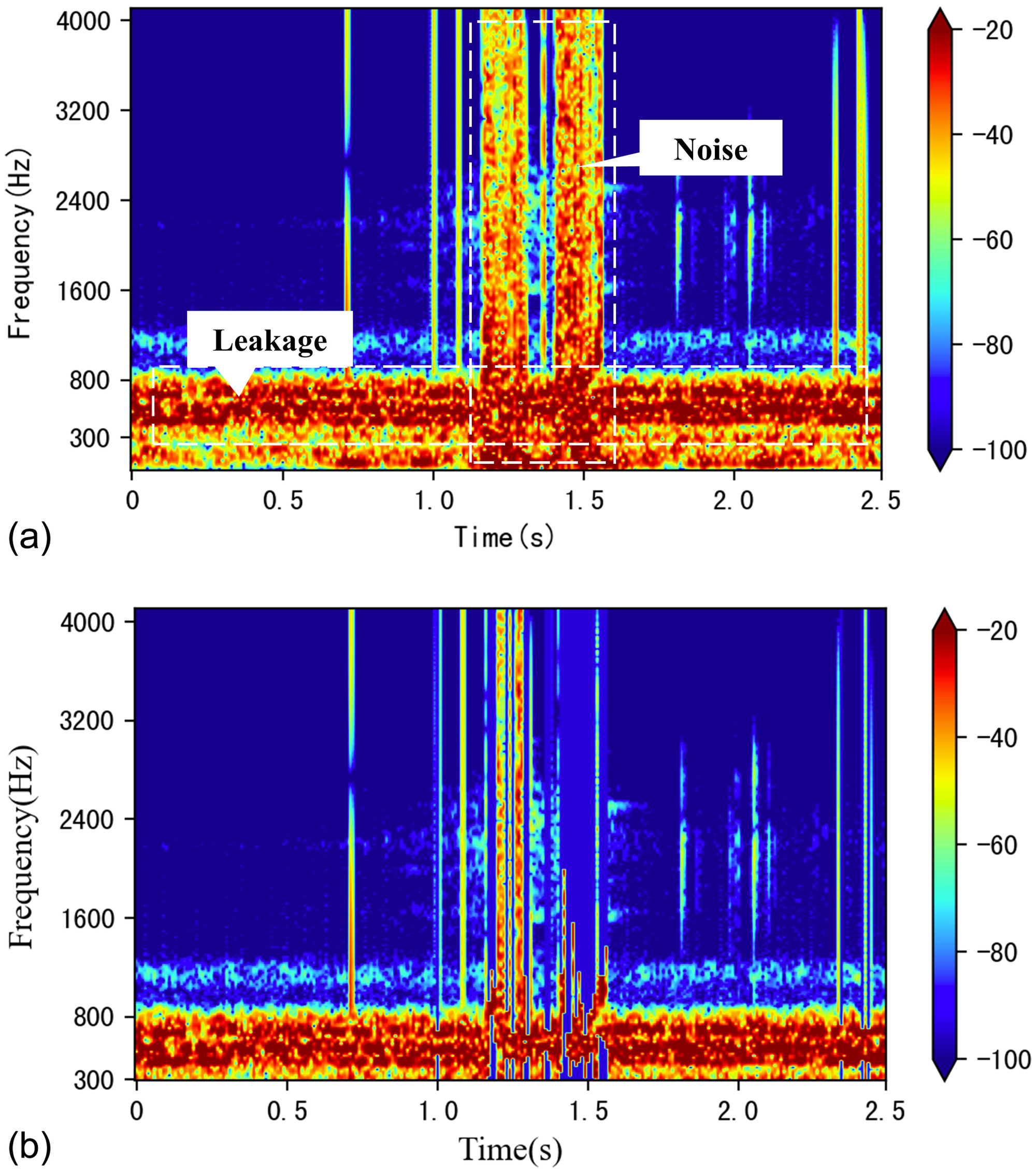
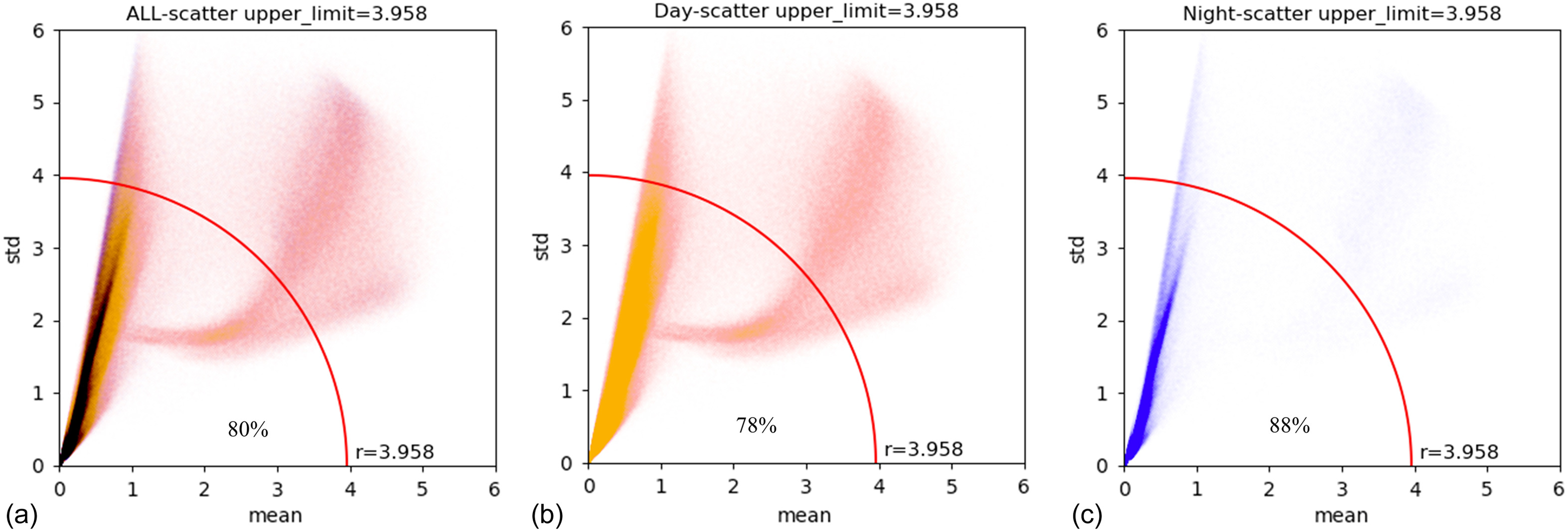
For random high background noise, the interference frame threshold is first determined. The mean and standard deviation of the FFT spectrum values for each frame of all 8,881 normal samples are calculated, and the Euclidean distance from the vector (mean, std) to the origin (0, 0) is computed to obtain a one-dimensional array of Euclidean distances Li (). Using the rule, the threshold is set as the 80th percentile value of 3.958 after sorting the array from smallest to largest [as shown in Fig. 7(a)]. The first 80% of the array is considered as normal frames, and the last 20% is considered as interference frames. Secondly, interference frames are identified and denoised. The mean and standard deviation of the spectral values for each frame of the audio after STFT are calculated, and if the Euclidean distance from the vector (mean, std) to the origin is greater than or equal to 3.958, the frame is identified as an interference frame and is denoised using peak retention. Two local peaks are retained for each interference frame, with a width of 6. As shown in Fig. 6(b), the processed log spectrogram is used as inputs for the PLS-ResNet18 model. As shown in Figs. 7(b and c), 78% of the daytime frames and 88% of the nighttime frames are within the threshold range, which is consistent with the fact that interference is more severe during the day than at night.
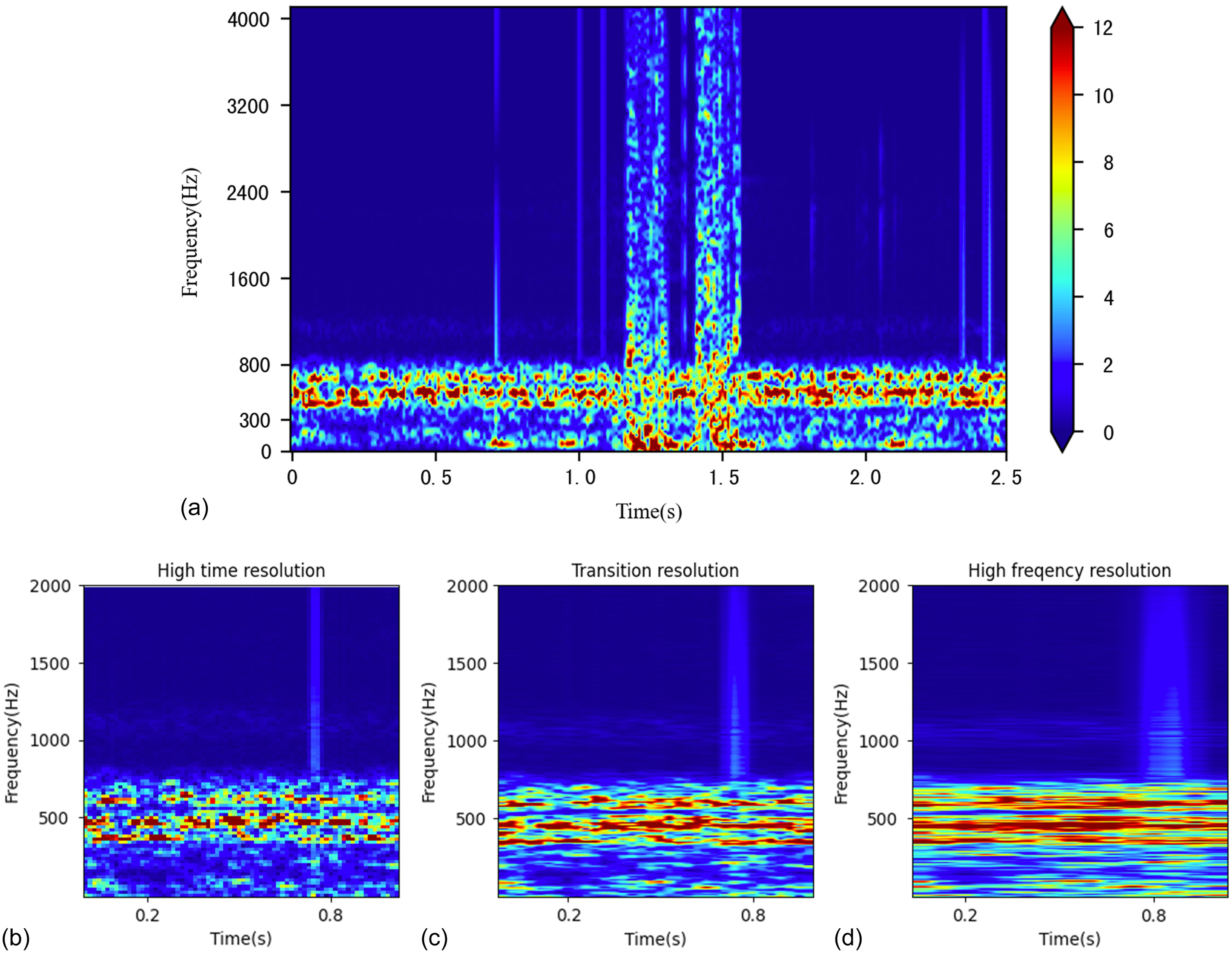
The time-frequency features of other classification models are extracted using the same data set. The linear spectrogram is shown in Fig. 8(a), and the parameters such as window function, FFT length, frame length, frame shift, and color mapping table are set the same as those for the log spectrogram. For the three resolution inputs figures of the TFCNN model shown in Figs. 8(b–d), a one-second audio signal is taken with a sampling frequency of 4,800 Hz. For high time resolution, the size of the spectrogram matrix is (100, 72); for intermediate time-frequency resolution, the size of the spectrogram matrix is (208, 34); and for high-frequency resolution, the size of the spectrogram matrix is (425, 15) (Guo et al. 2021).
Training and Evaluation of PLS-ResNet18 Model
The PLS-ResNet18 model was implemented using PyTorch 1.11.0+cu113 and Python 3.9.7. The ResNet18 model was constructed using the PyTorch framework, and the Adam optimizer was used to initialize the model parameters with a learning rate of 0.01 and weight decay set to . The MultiStepLR scheduler was used to adjust the learning rate to 0.1 times during training, at the 10th and 20th epochs, to gradually reduce the learning rate during training and avoid overfitting and oscillation. The cross-entropy loss function was used to define the loss, with a batch size of 256. ReLU was used as the activation function to speed up training and avoid gradient vanishing.
The model input is an audio file, and it is processed by constructing a data set class to read and preprocess audio and organize the data into a format that can be used by PyTorch. The specific steps are as follows: Read the audio from the audio path and obtain the audio array and the sampling rate. Perform frame segmentation on the audio array in the time domain with a frame length of 205, corresponding to a time range of 25 ms. Apply the Hann window as the window function. Set the frame shift to 83, corresponding to a time range of 10 ms. The obtained frames are transformed with FFT to obtain the amplitude spectrum Xi(k) for each frame, which is then combined into a two-dimensional matrix STFT. The result can be used to construct a linear spectrogram. The STFT matrix is squared and logarithmically transformed to obtain a two-dimensional matrix power with a unit of decibel (dB). It should be noted that the range of power values has a certain impact on the classification performance of the model. Increasing the minimum value is equivalent to filtering out signals with weak energy, which has a certain noise reduction effect. Here, the value range is set to [, ]. Finally, interference frame identification and peak retention denoising are used to generate a log spectrogram matrix with retained peaks.
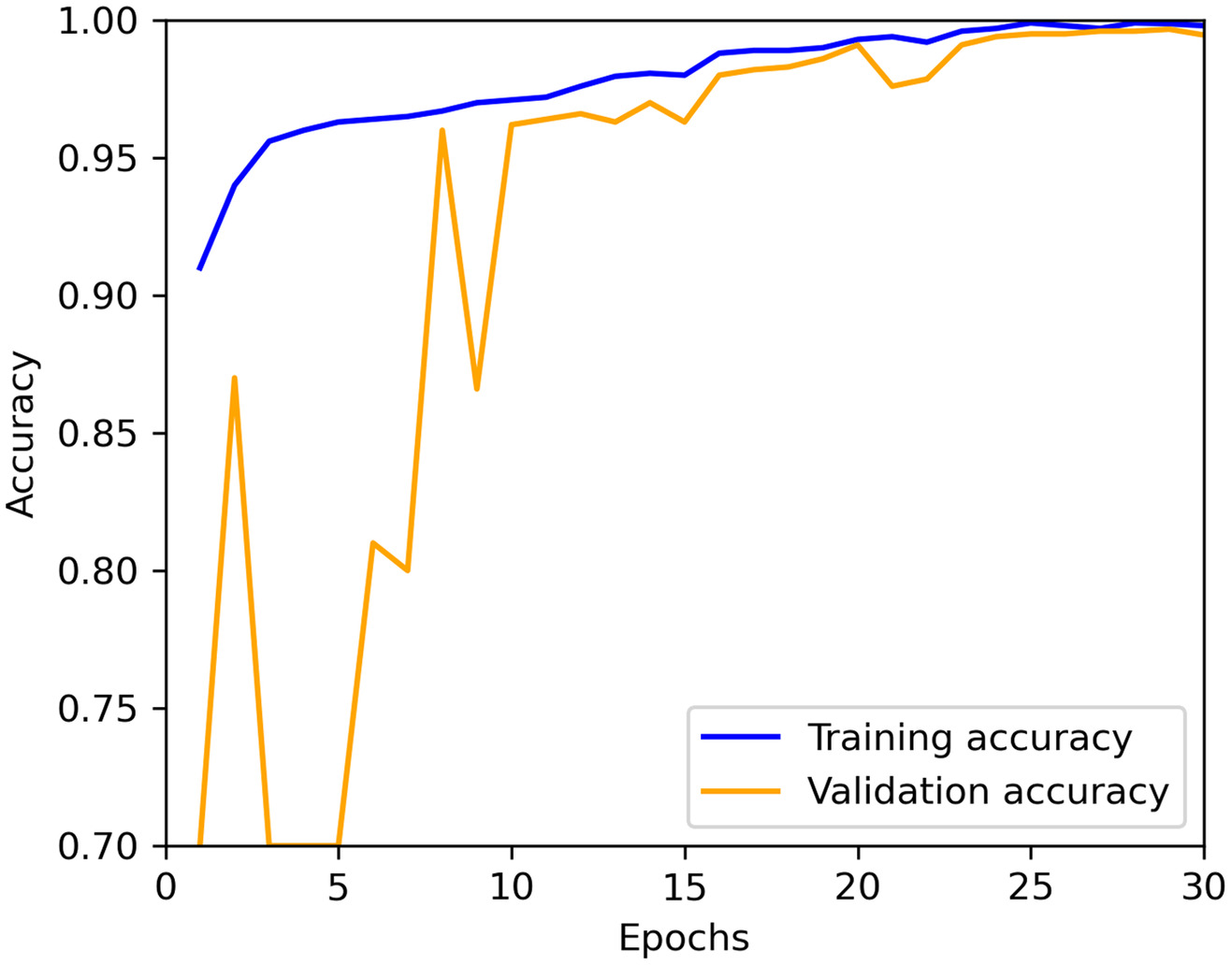
Fig. 9 shows the accuracy of the training set and the test set during the model training process, with both accuracies stabilizing at 0.993 after 16 epochs. The trained parameters were loaded, and the trained model was used to predict all data. The model accuracy was about 0.996, recall was approximately 0.990, precision was approximately 0.995, and F1-score was approximately 0.993, with all parameters exceeding 0.99.
Results and Discussion
Performance Evaluation
Table 1 summarizes the performance of different classification models on the entire data set, separately for daytime and nighttime. The results show that the accuracy (ACC) of the proposed method is 99.4% and the F1-score is 98.9%, both of which are significantly higher than other detection and classification methods. Compared with other experimental results obtained using different models, the proposed method has the following advantages: (1) the proposed method uses time-frequency features to characterize audio signals, which contain richer information than the single feature used by traditional STD-based detection algorithms and time-domain or frequency-domain features used in machine learning, (2) the proposed method uses a CNN model, which is good at processing complex nonlinear data and automatically extracting features, and can better reflect the changes of signals in the time and frequency domain, thus improving the accuracy and stability of leak detection, and (3) compared with the TFCNN model, the accuracy of the proposed model is improved by 5.3%, 5.0%, and 6.6% in the full day, daytime, and nighttime, respectively.
| Models | Period | TP | TN | FP | FN | ACC | Recall | Precision | F1-score |
|---|---|---|---|---|---|---|---|---|---|
| STD | Night | 340 | 1,320 | 152 | 206 | 0.822 | 0.623 | 0.691 | 0.655 |
| RF | All-day | 2,916 | 8,751 | 130 | 519 | 0.947 | 0.849 | 0.957 | 0.900 |
| Day | 2,459 | 7,288 | 121 | 430 | 0.946 | 0.851 | 0.953 | 0.851 | |
| Night | 457 | 1,463 | 9 | 89 | 0.951 | 0.837 | 0.981 | 0.903 | |
| XGBoost | All-day | 2,924 | 8,714 | 167 | 511 | 0.945 | 0.851 | 0.946 | 0.896 |
| Day | 2,464 | 7,253 | 156 | 425 | 0.944 | 0.853 | 0.940 | 0.895 | |
| Night | 460 | 1,461 | 11 | 86 | 0.952 | 0.842 | 0.977 | 0.905 | |
| TF-CNN | All-day | 3,021 | 8,573 | 308 | 414 | 0.941 | 0.879 | 0.907 | 0.893 |
| Day | 2,556 | 7,160 | 249 | 333 | 0.943 | 0.885 | 0.911 | 0.890 | |
| Night | 465 | 1,413 | 59 | 81 | 0.931 | 0.852 | 0.887 | 0.869 | |
| LS-ResNet18 | All-day | 2,561 | 6,639 | 2,242 | 864 | 0.747 | 0.748 | 0.555 | 0.637 |
| Day | 2,203 | 5,359 | 2,050 | 686 | 0.734 | 0.763 | 0.518 | 0.617 | |
| Night | 368 | 1,280 | 192 | 178 | 0.817 | 0.657 | 0.674 | 0.665 | |
| PLS-ResNet18 | All-day | 3,404 | 8,109 | 772 | 31 | 0.935 | 0.991 | 0.815 | 0.894 |
| Day | 2,862 | 6,676 | 733 | 27 | 0.926 | 0.991 | 0.796 | 0.883 | |
| Night | 542 | 1,433 | 39 | 4 | 0.979 | 0.993 | 0.933 | 0.962 | |
| Log S-ResNet18 | All-day | 3,187 | 8,876 | 5 | 248 | 0.979 | 0.928 | 0.998 | 0.962 |
| Day | 2,654 | 7,404 | 5 | 235 | 0.977 | 0.919 | 0.998 | 0.957 | |
| Night | 533 | 1,472 | 0 | 13 | 0.994 | 0.976 | 1.00 | 0.988 | |
| Log PS-ResNet18 | All-day | 3,369 | 8,872 | 9 | 66 | 0.994 | 0.981 | 0.997 | 0.989 |
| Day | 2,828 | 7,401 | 8 | 61 | 0.993 | 0.979 | 0.997 | 0.988 | |
| Night | 541 | 1,471 | 1 | 5 | 0.997 | 0.991 | 0.998 | 0.994 |
From the ablation experiment results, it is found that (1) when the linear spectrogram is replaced by the log spectrogram for the same CNN model, the model accuracy is improved by 23.2%. This proves that the log spectrogram has stronger representation ability, a wider dynamic range, and can better reflect the signal intensity and energy distribution, which greatly enhances the gain of the model, (2) when peak noise reduction is applied to the linear spectrogram, the model accuracy is improved by 18.8%, indicating that peak retention denoising has a significant effect and can effectively suppress interference, greatly improving the detection ability, and (3) when both the log spectrogram and denoising are used simultaneously, the accuracy is improved by 24.7%, indicating that these two improvement methods can be used together, and the effect is the best.
Comparing the experimental data of daytime and nighttime, it can be seen that the indicators at nighttime are generally better than those during the daytime. Comparing TFCNN and S-ResNet18, it can be seen that although the signal duration and sampling frequency are increased, the representation ability of the single-resolution linear spectrogram for leak signals is still not strong enough, and interference signals have a huge impact on it. In addition, the recall rate of most models is lower than the precision rate, because detecting weak leaks is difficult both during the day and at night, and weak signal features are not obvious and are easily missed due to interference.
Comparing the daily detection metrics (ACC, Recall, Precision, and F1-score) of the seven models in Table 1, the following observations can be made: (1) the machine learning methods RF and XGBoost exhibit similar metrics, indicating a tendency to classify weak leaks as normal during detection, (2) PLS-ResNet18 shows improvement in all metrics compared to LS-ResNet18, suggesting significant noise reduction during the daytime using the peak denoising method, and (3) the log PS-ResNet18 model demonstrates significant improvement in daily detection performance by inheriting the high recall rate of PLS-ResNet18 and the high precision of log S-ResNet18.
Influence of Noise on Model
Figs. 10 and 11 show various time-frequency domain spectrograms for normal and leak states. Upon comparison, it is easy to find that due to the existence of a large amount of interference signals, the graphics corresponding to the two states are quite similar, and only the log P-Spectrogram shows a significant difference between the two states, which makes only the log PS-ResNet18 method correctly identify these two states. The high-energy background noise exhibits intense and sustained performance, and its high-intensity energy covers the entire log spectrogram, making leak detection difficult in this situation. This is also the main reason for the FP rate of daytime leak detection. The leak signal is continuous in the time domain and has consistent high-level intensity in the frequency domain, with a relatively narrow frequency band (400–800 Hz).
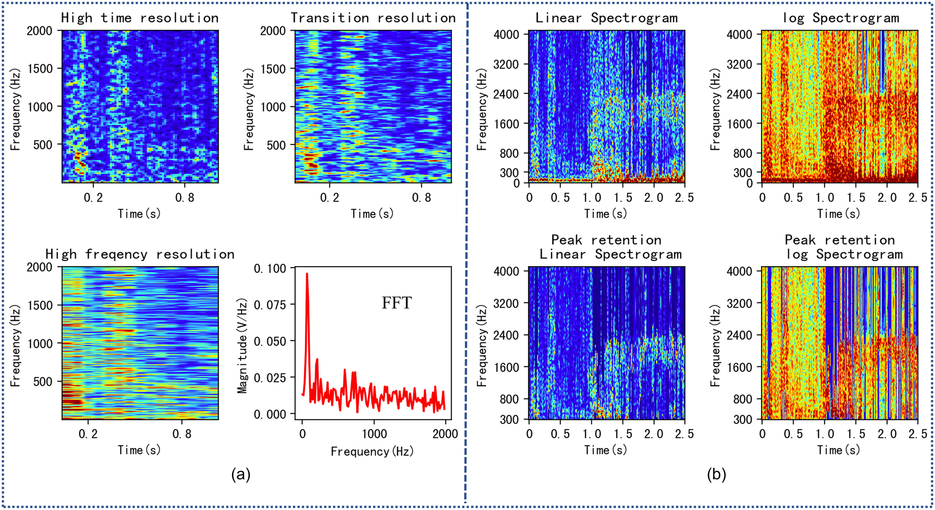
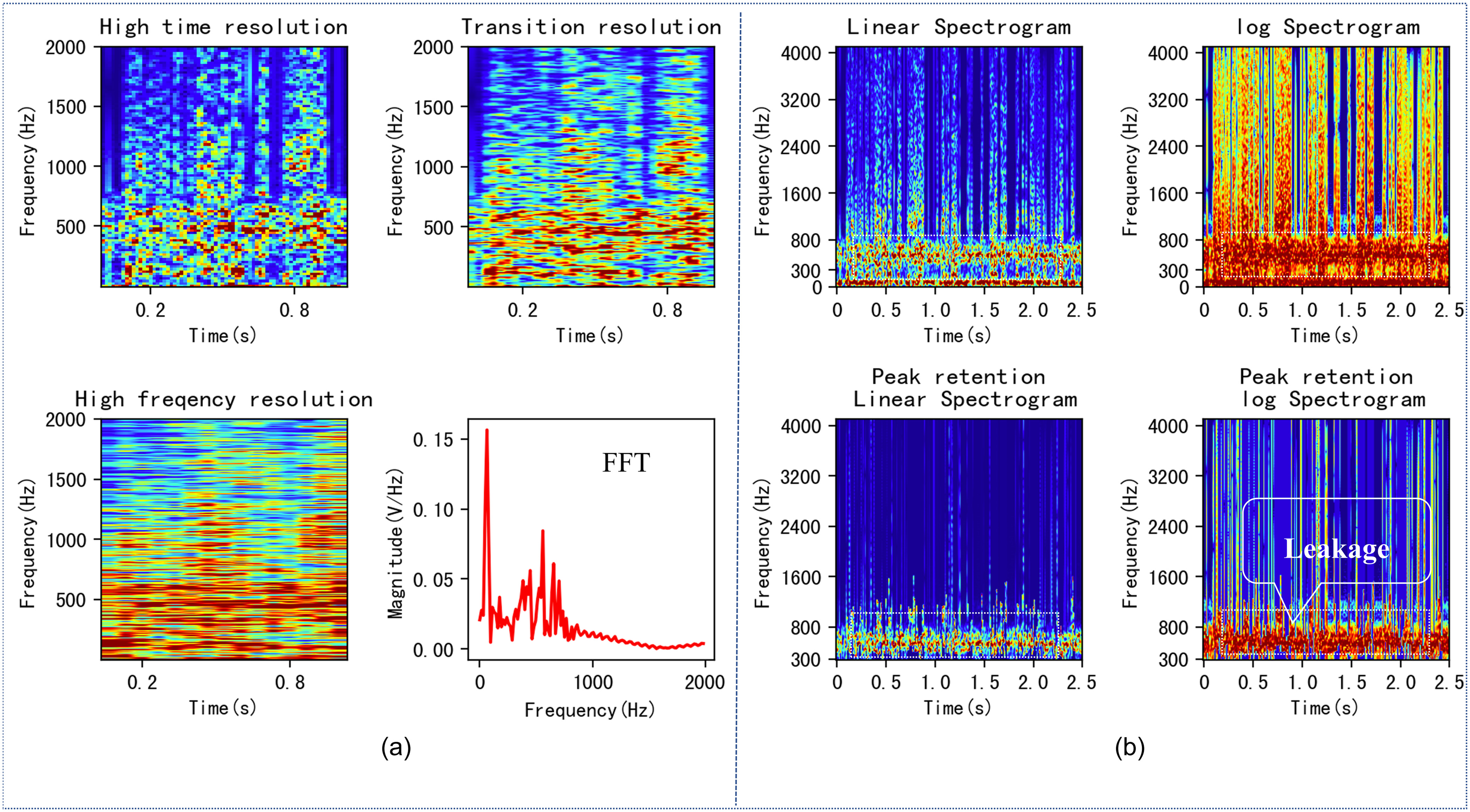
To address the high-energy noise in the low-frequency band, the TFCNN model uses a bandpass filter with a frequency response range of 100 to 2,000 Hz to reduce interference. For cases where the interference frequency band and leak response frequency band are different, we believe that it is unnecessary to process the unrelated frequency bands, and the CNN model can automatically distinguish between the interference and leak frequency bands. If peak preservation is required, processing of sustained low-frequency high-energy noise should be performed before the operation. In this paper, we use the truncation method to achieve better noise reduction results.
Application of Log PS-ResNet18 Model
In this paper, we trained and tested multiple classification models using real round-the-clock data from WDS to verify their performance in actual environments. Our experimental results show that the log PS-ResNet18 model performs the best in practical applications and has the highest detection accuracy. Therefore, we recommend deploying this model on the server-side for intelligent detection. Specifically, we can deploy round-the-clock noise loggers in the distribution network and use multiple features extracted from the audio signals (such as STD, CF, and ZCR) for leak discrimination. These features can be calculated using simple models such as RF and XGBoost for low-power initial detection. Then, the suspicious audio signals can be transmitted to the cloud platform for secondary recognition using the log PS-ResNet18 model to further improve detection accuracy.
We monitored part of the water distribution network in LS City using the above devices, which includes pipes with diameters ranging from DN100 to DN400, and collected 518 leak samples and 1,316 normal samples (a total of 1,834 samples collected by 11 noise loggers for ). After testing, there were seven FNs, and the rest of the samples were correctly detected, with an accuracy rate of 99.6%, a recall rate of 98.7%, a precision rate of 100%, and an F1-score of 99.3%. This indicates that the proposed intelligent detection model has high accuracy in practical applications. After examination, the seven FNs corresponded to weak leaks in daytime environments, where the leak signal characteristics were not obvious, resulting in detection errors. This also indicates that detecting weak leaks during the daytime remains a challenge in this field. Further breakthroughs and upgrades are needed in both algorithms and hardware instrumentation to solve this problem.
Conclusions
This study combined logarithmic spectrograms and the ResNet18 model to detect leaks in real round-the-clock WDS. Unlike most studies that do not consider actual field conditions, this research developed and selected feature extraction and detection methods for leak detection in noisy daytime environments, and proposed a CNN leak detection method based on peak-preserved denoising log spectrograms suitable for practical/field situations. Using the peak-preserved log spectrogram as the feature of the leak signal, the ResNet18 model was used for leak detection and compared with other models. The following conclusions were drawn:
1.
Logarithmic spectrograms can better highlight the characteristics of leak and interference signals, with a wider dynamic range and more effectively emphasize the time-frequency characteristics of signals. We also designed a reasonable color mapping and selected an appropriate matrix value range based on signal characteristics, fully leveraging the advantages of time-frequency domain.
2.
By analyzing the log spectrogram, it was confirmed that leak signals have consistent high-level intensity in frequency, with a relatively narrow distribution range, while random high-energy background noise often has high-intensity peaks in frequency with a wide distribution range, showing strong randomness.
3.
Daytime interference is more abundant and energetic, belonging to a low SNR environment, and the detection indicators of all models are lower than those in nighttime environments. Achieving round-the-clock detection requires reducing the influence of random high-energy noise interference during the daytime.
4.
Nonstationary noise such as traffic noise significantly affects leak detection. To reduce interference, we used frame-based approaches to identify and preserve the peak values of interference frames to achieve denoising effects.
5.
Machine learning models have a higher dependence on feature selection and can achieve higher detection performance. Among deep learning models, the model based on a single linear spectrogram has the worst performance, while models based on three resolution linear spectrograms show significant improvement in detection results. The model based on log spectrograms performs better, and the model based on an improved log spectrogram has the best performance. This model is expected to achieve round-the-clock leak detection in actual WDS.
Future work will develop practical applications based on this model, integrate them with cloud platforms, and conduct comparative studies with industry best practices to verify the accuracy and efficiency of the proposed method. In addition, research on detecting weak signals and leak localization will be conducted.
Data Availability Statement
Some or all data, models, or code that support the findings of this study are available from the corresponding author upon reasonable request: (1) sample data including audio files and labels, (2) models, and (3) codes.
Acknowledgments
This work was supported by the National Natural Science Foundation of China (U1509205).
References
Adedeji, K. B., Y. Hamam, B. T. Abe, and A. M. Abu-Mahfouz. 2017. “Towards achieving a reliable leakage detection and localization algorithm for application in water piping networks: An overview.” IEEE Access 5 (Sep): 20272–20285. https://doi.org/10.1109/ACCESS.2017.2752802.
Bhangale, K., and K. Mohanaprasad. 2022. Speech emotion recognition using mel frequency log spectrogram and deep convolutional neural network, 241–250. New York: Springer.
Chan, T. K., C. S. Chin, and X. Zhong. 2018. “Review of current technologies and proposed intelligent methodologies for water distributed network leakage detection.” IEEE Access 6 (Mar): 78846–78867. https://doi.org/10.1109/ACCESS.2018.2885444.
Cody, R. A., B. A. Tolson, and J. Orchard. 2020. “Detecting leaks in water distribution pipes using a deep autoencoder and hydroacoustic spectrograms.” J. Comput. Civ. Eng. 34 (2): 04020001. https://doi.org/10.1061/(ASCE)CP.1943-5487.0000881.
Dennis, J., H. D. Tran, and H. Li. 2010. “Spectrogram image feature for sound event classification in mismatched conditions.” IEEE Signal Process Lett. 18 (2): 130–133. https://doi.org/10.1109/LSP.2010.2100380.
Diao, X., J. Jiang, G. Shen, Z. Chi, Z. Wang, L. Ni, A. Mebarki, H. Bian, and Y. Hao. 2020. “An improved variational mode decomposition method based on particle swarm optimization for leak detection of liquid pipelines.” Mech. Syst. Signal Process. 143 (May): 106787. https://doi.org/10.1016/j.ymssp.2020.106787.
El-Abbasy, M. S., F. Mosleh, A. Senouci, T. Zayed, and H. Al-Derham. 2016. “Locating leaks in water mains using noise loggers.” J. Infrastruct. Syst. 22 (3): 04016012. https://doi.org/10.1061/(ASCE)IS.1943-555X.0000305.
Fan, H., S. Tariq, and T. Zayed. 2022. “Acoustic leak detection approaches for water pipelines.” Autom. Constr. 138 (Mar): 104226. https://doi.org/10.1016/j.autcon.2022.104226.
Fantozzi, M., and E. Fontana. 2001. “Acoustic emission techniques: The optimum solution for leakage detection and location in water pipelines.” Insight 43 (2): 105–107.
Fuchs, H. V., and R. Riehle. 1991. “Ten years of experience with leak detection by acoustic signal analysis.” Appl. Acoust. 33 (1): 1–19. https://doi.org/10.1016/0003-682X(91)90062-J.
Guo, C., K. Shi, and X. Chu. 2022. “Cross-correlation analysis of multiple fibre optic hydrophones for water pipeline leakage detection.” Int. J. Environ. Sci. Technol. 19 (1): 197–208. https://doi.org/10.1007/s13762-021-03163-y.
Guo, G., X. Yu, S. Liu, Z. Ma, Y. Wu, X. Xu, X. Wang, K. Smith, and X. Wu. 2021. “Leakage detection in water distribution systems based on time–frequency convolutional neural network.” J. Water Resour. Plann. Manage. 147 (2): 04020101. https://doi.org/10.1061/(ASCE)WR.1943-5452.0001317.
He, K., X. Zhang, S. Ren, and J. Sun. 2016. “Deep residual learning for image recognition.” In Proc., IEEE Conf. on Computer Vision and Pattern Recognition, 770–778. New York: IEEE. https://doi.org/10.1109/cvpr.2016.90.
Kang, J., Y.-J. Park, J. Lee, S.-H. Wang, and D.-S. Eom. 2017. “Novel leakage detection by ensemble CNN-SVM and graph-based localization in water distribution systems.” IEEE Trans. Ind. Electron. 65 (5): 4279–4289. https://doi.org/10.1109/TIE.2017.2764861.
Lim, J. 2014. Underground pipeline leak detection using acoustic emission and crest factor technique, 445–450. New York: Springer.
Martini, A., A. Rivola, and M. Troncossi. 2018. “Autocorrelation analysis of vibro-acoustic signals measured in a test field for water leak detection.” Appl. Sci. 8 (12): 2450. https://doi.org/10.3390/app8122450.
Martini, A., M. Troncossi, and A. Rivola. 2015. “Automatic leak detection in buried plastic pipes of water supply networks by means of vibration measurements.” Shock Vib. 2015 (Jan): 1–13. https://doi.org/10.1155/2015/165304.
Mounce, S. R., J. B. Boxall, and J. Machell. 2010. “Development and verification of an online artificial intelligence system for detection of bursts and other abnormal flows.” J. Water Resour. Plann. Manage. 136 (3): 309–318. https://doi.org/10.1061/(ASCE)WR.1943-5452.0000030.
Odusami, M., R. Maskeliūnas, R. Damaševičius, and T. Krilavičius. 2021. “Analysis of features of Alzheimer’s disease: Detection of early stage from functional brain changes in magnetic resonance images using a finetuned ResNet18 network.” Diagnostics 11 (6): 1071. https://doi.org/10.3390/diagnostics11061071.
Shukla, H., and K. Piratla. 2020. “Leakage detection in water pipelines using supervised classification of acceleration signals.” Autom. Constr. 117 (Sep): 103256. https://doi.org/10.1016/j.autcon.2020.103256.
Tariq, S., B. Bakhtawar, and T. Zayed. 2022. “Data-driven application of MEMS-based accelerometers for leak detection in water distribution networks.” Sci. Total Environ. 809 (Feb): 151110. https://doi.org/10.1016/j.scitotenv.2021.151110.
Wang, Z., X. He, H. Shen, S. Fan, and Y. Zeng. 2022. “Multi-source information fusion to identify water supply pipe leakage based on SVM and VMD.” Inf. Process. Manage. 59 (2): 102819. https://doi.org/10.1016/j.ipm.2021.102819.
Xin, M., and L. Wu. 2020. “Using multi-features to partition users for friends recommendation in location based social network.” Inf. Process. Manage. 57 (1): 102125. https://doi.org/10.1016/j.ipm.2019.102125.
Zhou, B., V. Lau, and X. Wang. 2019. “Machine-learning-based leakage-event identification for smart water supply systems.” IEEE Internet Things J. 7 (3): 2277–2292. https://doi.org/10.1109/JIOT.2019.2958920.
Information & Authors
Information
Published In

Journal of Water Resources Planning and Management
Volume 150 • Issue 6 • June 2024
Copyright
This work is made available under the terms of the Creative Commons Attribution 4.0 International license, https://creativecommons.org/licenses/by/4.0/.
History
Received: Jun 2, 2023
Accepted: Jan 9, 2024
Published online: Mar 27, 2024
Published in print: Jun 1, 2024
Discussion open until: Aug 27, 2024
Authors
Metrics & Citations
Metrics
Citations
Download citation
If you have the appropriate software installed, you can download article citation data to the citation manager of your choice. Simply select your manager software from the list below and click Download.