Water Management for Conservation and Ecosystem Function: Modeling the Prioritization of Source Water in a Working Landscape
Publication: Journal of Water Resources Planning and Management
Volume 149, Issue 5
Abstract
Conservation in working landscapes is an important aspect of stream restoration. Landowners with agricultural water rights are increasingly adding instream flow as a beneficial use of their allocated water. However, stream restoration projects commonly focus on the quantity of water dedicated to the environment and overlook water quality. For cold-water ecosystems, the preservation of natural thermal regimes is a key to conservation efforts in the face of a changing climate. This study explored the effects of increasing stream flow using alternative water sources (e.g., instream runoff versus offchannel springs) to enhance cold-water stream habitat on a working cattle ranch. Using empirical data to create a steady-state stream flow and water temperature model, we evaluated temperature benefits and management trade-offs for ecological and agricultural water use. The modeled results showed that the source of water and the method used to deliver water to the channel affected the quality and extent of cold-water habitat. Offchannel spring water cooled 7-day average maximum temperatures and 7-day average mean temperatures by as much as 3.7°C and 2.9°C, respectively, but only when potential offchannel aquatic habitat was sacrificed for mainstem habitat. When offchannel, spring-fed habitat was provided, the value of spring water to the main channel decreased. Our findings suggest that source water thermal quality is of paramount importance for enhancing ecosystem function and improving cold-water habitat in working landscapes. In addition, the restoration of a historic spring channel may provide added ecosystem benefits by enhancing aquatic habitat for cold-water species.
Practical Applications
In the western United States, understanding the best possible uses for high-quality cold-water sources may provide the greatest benefits to the environment and adjacent working landscapes. Whereas water purchases and leases tend to focus on water quantity, this study could direct such investments toward higher value sources for the environment. In places like California, where drought has resulted in water right curtailments for agricultural diverters, understanding the best uses for high quality cold water compared with other sources can provide the greatest benefits to both agriculture and the environment.
Introduction
With 45% of streams and rivers in the United States in a state of impairment (USEPA 2000), stream restoration has become a major focus in environmental management and hydrologic science (Wohl et al. 2005). Extinction rates for freshwater species are five times greater than they are for terrestrial fauna; this can be attributed to habitat loss associated with shifts in water quality (including thermal regimes) and flow (Ricciardi and Rasmussen 1999). To reverse the loss of critical freshwater habitat and restore the ecological integrity of streams throughout the western United States, actively managing impaired rivers is vital (Bernhardt et al. 2007; Downs et al. 2011).
Cold-water spring-fed streams have recently been recognized for their ecological value in producing stable flows and temperatures (Isaak et al. 2015; Lusardi et al. 2016, 2021; Willis et al. 2017, 2021) and robust ecosystems (Lusardi et al. 2020, 2021). The restoration and maintenance of springs and spring-fed rivers is fundamental to the conservation of cold-water biota, including keystone species such as salmonids (Isaak et al. 2015; Lusardi et al. 2016, 2020, 2021). Conservation efforts that seek to maintain instream flows and temperature during crucial migration and rearing periods, particularly within working landscapes, have proven to be successful elsewhere (Nichols et al. 2010; Willis et al. 2016).
Despite recent successes, maintaining cold-water habitat across working landscapes may be more critical now than ever. Private agricultural lands account for 52% of the total land area in the United States and provide habitat for 85% of all federally listed endangered species (Kamal et al. 2015). However, less than 1% of private lands are currently used to enhance habitat, particularly where freshwater resources are concerned (Kamal et al. 2015). To complicate matters, water management is commonly a source of disunity between freshwater conservationists and private landowners (Garibaldi et al. 2021), and current climate projections suggest that nearly 40% of cold-water habitat across the United States will be lost if present trends continue (Mohseni et al. 2003). In drought-prone northern California, limited water resources, private water rights allocations, and the inefficient transport and use of natural water resources often leads to complications in water resources management (Vissers 2017).
The identification and preservation of cold-water habitats is vital to the future success of dependent species (Isaak et al. 2015; Fullerton et al. 2018). The vulnerability of these species has led to numerous studies assessing the potential thermal effects of a warming climate on freshwater fish habitat (Eaton and Scheller 1996; Isaak et al. 2018). For species with complex migratory life histories, like salmon, the uncertainties surrounding the effects of a warming climate are even greater, because these species are highly sensitive to thermal changes and fluctuations (Crozier et al. 2008; Lestelle 2007). Water temperatures above certain thresholds have been shown to reduce reproductive success and limit the growth and survival of numerous native fishes, particularly those that are dependent on cold water (Fenkes et al. 2016; Welsh et al. 2001). Juvenile salmon, like other cold-water adapted species, require cold water during their stream residency period, making the quality of these habitats critical to population success.
To recover and conserve cold-water species within working landscapes, it is imperative to utilize cold-water resources effectively and efficiently (Isaak et al. 2018). Restoration on private, working lands can improve habitat connectivity, range, and quality to help limit impairment associated with climate change (Seavy et al. 2009), and studies have shown that the restoration of spring-fed cold-water habitats on private agricultural lands is beneficial to cold-water fishes (Null et al. 2010; Nichols et al. 2020). However, many river restoration strategies focus on improving habitats through changes to volume or timing of flow (e.g., Kiernan et al. 2012; Null et al. 2017; Willis et al. 2016, 2022). Fewer studies have assessed the ecological trade-offs of dedicating water rights to beneficial instream uses of comparable volume but substantially different water quality. Specifically, in regions where both instream runoff and offchannel springs are diverted for agricultural use, the relative value of each water source in enhancing thermal and water quality conditions and flow volumes has not been explored.
In this study, we modeled the stream temperature outcomes of alternative water management strategies to examine the efficacy of using surface runoff or spring-fed water rights dedication to support a cold-water ecosystem, specifically during the summer period for juvenile salmonids. Our aim was to (1) assess stream temperature outcomes and differences between surface runoff and offchannel spring-fed water rights used to enhance stream temperature; and (2) better understand the trade-offs in prioritizing thermal regimes and habitat in a runoff stream versus a spring-fed tributary channel. The results of this study can be used to prioritize conservation efforts for water rights transfers that enhance both the quantity and quality of instream aquatic habitat within working landscapes.
Methods
Study Area
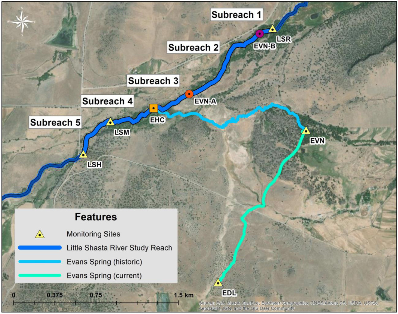
Evans Spring is a natural cold-water spring located in the Shasta River watershed of northern California. This watershed supports the southernmost population of southern Oregon/northern California coast (SONCC) coho salmon (Oncorhynchus kisutch), a species listed as threatened under the Federal and California endangered species acts. Historically, Evans Spring was a tributary to the Little Shasta River, contributing approximately of mean annual flow. Currently, Evans Spring is diverted for agricultural use and does not directly contribute to the Little Shasta River. Recent studies have suggested that the foothills of the Little Shasta River may still provide suitable cold-water habitat for oversummering salmonids (SVRCD 2013; Nichols et al. 2016), making the upper reaches of this river an area of interest for conservation.
The 2.2-km reach of the Little Shasta River that was modeled for this study is located just upstream of a surface water diversion [Little Shasta River at Hart-Haight diversion (LSH); see Fig. 1]. During summer baseflow, this diversion becomes a point of hydrologic disconnection to downstream reaches. Reaches downstream of this diversion are seasonally disconnected, while reaches upstream of this diversion remain entirely connected and potentially provide oversummering habitat for cold-water fishes. The historical point of connection of Evans Spring to the Little Shasta River is also located within this reach.
Stream Temperature Modeling
We used stream temperature metrics to assess the relationship between Evans Spring and stream temperatures in the Little Shasta River. Water temperature metrics for this study were based on thresholds for juvenile coho salmon habitat utilization from Welsh et al. (2001), with a maximum weekly average temperature (MWAT) of 17.6°C and a maximum weekly maximum temperature (MWMT) of 18.1°C.
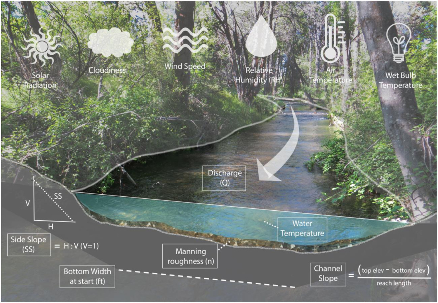
A stream temperature model was developed to simulate alternative management scenarios. The Water Temperature Transaction Tool version 0.9n_1 (W3T) was developed as an open-access, open-code spreadsheet model to track individual diversions or water transfers through a stream and evaluate how they influence water temperature over short-term (1–7-day) periods (Watercourse Engineering 2013). This steady-state stream model allows the assessment of the thermal impacts of various alterations to a stream, including tributary inflows and irrigation diversions, on an hourly time step.
Three separate models were required to simulate alternative management strategies for Evans Spring. The first model was created to simulate water temperatures within the study reach of the Little Shasta River. Initially, observed hourly stream temperature data for the Little Shasta River (LSH) was assessed to identify a 7-day period with high maximum daily temperatures and stable stream flow. Next, publicly accessible data were assembled, reviewed, and used to implement and calibrate the model. A second W3T was created to model the current Evans Spring channel, and a third W3T model was created to simulate the effects of the historical channel when reconnected and restored with riparian planting. Last, the results from both current and historical Evans Spring models were applied as inflows to the original Little Shasta model to simulate outgoing temperatures for each management strategy. Details of the equipment and locations used for field monitoring, sources of publicly accessed data, and model performance targets and scenario analysis are provided in the following.
Field Monitoring and Data Collection
Water temperature was monitored in the Little Shasta River and Evans Spring from mid-June to late-September of 2020 to capture high temperatures during the baseflow period. Little Shasta River remote station (LSR) stage, flow, and temperature were monitored via a remote station operated by The Nature Conservancy. At monitoring sites LSH and Evans Spring (EVN), Solinst Levelogger Edge M10s (Solinst Canada Ltd., Georgetown, Ontario, Canada) were installed instream within PVC stilling wells to monitor water temperature and stage at 30-min intervals. The temperature sensors on these loggers have an accuracy of and an operating range of to 80°C; the stage sensors have an accuracy of . After estimating the length of the Evans Spring historical channel using publicly accessible remote images via Google Earth version 7.3.4.8642, a HOBO U22 Water Temperature Pro v2 data logger (Onset Computer Corporation, Bourne, Massachusetts) was installed in the current channel [Evans Spring diversion lower (EDL)] at the same measured distance. This logger also recorded water temperatures in 30-min intervals with an accuracy of . In addition, to place the analysis in a wider context, snowpack data from a publicly accessible database was used to determine hydrologic year type (e.g., dry, normal, or wet).
Model Implementation
Along with the collection of field data, additional data were required to implement each model. These data were collected through multiple sources, including publicly accessible data from permanent weather stations, satellite imagery, and estimated values based on field observations of the study reach (see Table 1). To allow for a more detailed representation of variations in channel characteristics, each modeled reach was divided into multiple subreaches based on the locations of monitoring sites, diversions, and tributaries or on notable changes in slope or land cover (see Table 2).
| Data | Source | Timestep | Units |
|---|---|---|---|
| Water temperature | |||
| Little Shasta River | Remote stations at LSR and LSH | 15 min | °C |
| Evans Spring | Dataloggers at EVN and EDL | 15 min | °C |
| Discharge | |||
| Little Shasta River | Remote stations at LSR and LSH | 15 min | |
| Evans Spring | Dataloggers at EVN and EDL | 15 min | |
| Channel geometry | |||
| Bottom width at start | Estimated based on field observations | N/A | ft |
| Side slope (SS) | Calculated based on Google Earth imagery | N/A | N/A |
| Channel slope | Calculated based on Google Earth imagery | N/A | N/A |
| Manning roughness () | Estimated based on field observations | N/A | N/A |
| Riparian vegetation | Estimated based on field observations | N/A | N/A |
| Meteorological | |||
| Air temperature | Remote station at Big Springs Creek | 1 h | °C |
| Cloudiness | Calculated based on solar radiation | 1 h | N/A |
| Wind speed | Remote station at Big Springs Creek | 1 h | mph |
| Relative humidity (RH) | Remote station at Big Springs Creek | 1 h | % |
| Wet bulb temperature | Calculated based on RH and air temp | 1 h | °C |
| Subreach | Site | Name | River kilometer | Type |
|---|---|---|---|---|
| 1 | LSR | Upstream property boundary | 23.51 | Upstream boundary |
| 2 | EVN-A | Evans Pipe Scenario A | 23.54 | Tributary |
| 3 | EVN-B | Evans Pipe Scenario B | 26.94 | Tributary |
| 4 | EHC | Evans historical channel | 26.96 | Tributary |
| 5 | LSM | Musgrave diversion | 28.69 | Diversion |
| — | LSH | Hart-Haight diversion | 29.74 | Downstream boundary |
Note: Each subreach is bordered by monitoring sites as shown.
Meteorological data, including relative humidity, solar radiation, air temperature, and wind speed, were obtained from a remote monitoring station at Big Springs Creek (coordinates: 41.6018075, ). This station is located approximately 14.5 km south-southwest from the Little Shasta River study reach. Wet bulb temperatures were calculated based on relative humidity and air temperature measurements, and cloud cover was calculated based on daily maximum solar radiation measurements.
Shade data for each subreach was estimated using Google Earth imagery. Shade features were generalized as either vegetation (e.g., deciduous trees, shrubs, grassland, etc.) or topographic (e.g., cutbank) and were further refined by type and direction relative to the course of the stream channel. Each shade feature was also associated with defined values for height and percent density.
Channel geometry was estimated based on Google Earth imagery and qualitative field observations of the study reach. The bottom width of the channel describes the bottom of the wetted portion of the channel at a specified flow and was estimated based on field observations of channel width. Side slope describes the slope of the sides of the wetted channel and was estimated based on elevation data from Google Earth imagery along the banks of the monitoring reach. Channel slope describes the slope of the longitudinal profile of the channel and was also calculated based on Google Earth elevations of the top and bottom of the study reach. Last, channel roughness describes the size and texture of the sediment on the bed of the channel, which was estimated based on guidelines from Chow (1959) and field observations. A summary of all channel geometry parameters used in the model is shown in Fig. 2.
Model Calibration
Model performance was quantified based on guidelines established in Moriasi et al. (2007). Performance metrics included percent bias (PBIAS), mean absolute error (MAE), and root mean squared error (RMSE). Percent bias (PBIAS) was calculated to show the percent of error between observed and simulated temperatures. Mean absolute error (MAE) was calculated to show the average error between observed and simulated temperature data. Root-mean square error (RMSE) was calculated to assess for potential larger errors. The goal for the MAE and RMSE statistics were for the results to be within half of the standard deviation between the observed and simulated temperatures, and the goal for PBIAS was to get as close to 0.00% as possible. Positive PBIAS values indicate an underestimation bias, and negative values indicate an overestimation bias.
Model Application: Alternatives Analysis
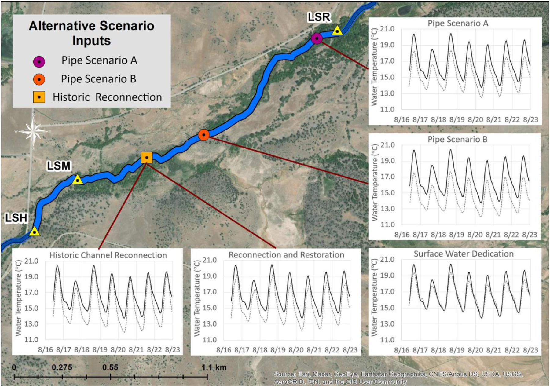
After calibrating baselines for all three study reaches (Little Shasta River, Evans Spring historical, Evans Spring current), five alternative water management scenarios were simulated. To quantify the short-term and potential long-term effects of reconnecting Evans Spring using its natural channel to convey spring water, the historical channel was modeled given current and restored (e.g., following riparian restoration planting) riparian vegetation conditions. Next, to quantify the maximum thermal benefit of Evans Spring on the Little Shasta River, two scenarios were simulated in which Evans Spring water was piped directly to two locations in Little Shasta River. Pipe Scenario A involved piping water from near the source of Evans Springs directly to the Little Shasta River, close to the top of the property boundary. Pipe Scenario B involved piping Evans Spring water from near the spring source to a point that would entail the shortest distance of piping to the Little Shasta River. For both pipe scenarios, no temperature gain was assumed for the Evans Spring water as it flowed from its source to the pipe outlet. Observed water temperatures from near the source of Evans Spring (EVN) were applied to the Little Shasta River model to simulate the addition of piped spring water to the study reach. Last, to quantify the effects of surface water runoff, streamflow at the upstream boundary was increased by , with no contribution from Evans Spring. The effects of each scenario were assessed based on the 7-day minimum, mean, and maximum stream temperatures at the downstream boundary of the Little Shasta River study reach.
Results
Observed Data
The date range of August 16–22, 2020, was selected for this study based on the assessment of 7-day average maximum daily temperatures in the Little Shasta River at the downstream boundary site LSH (see Fig. 3). This was the second-warmest date range during the monitoring period, and the dates also correlated with stable stream stages at LSR and LSH. The combination of high daily maximum stream temperatures and stable flow indicated that summer baseflows were observed during this period and that there were minimal effects from surface water diversions. The elevated stream temperature conditions and steady observed flows made this period well-suited for representation by the steady state W3T models.
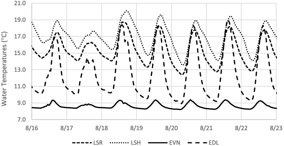
Based on assessments of snow-water content from the nearest snowpack monitoring station, 2020 was a normal water year for this region. A baseflow of was used as the inflow at the top of the reach (LSR); was diverted from the stream at Little Shasta River at Musgrave (LSM), leaving of outflow from the reach (LSH). Flow produced from Evans Spring was based on manually measured flows during the study period.
Model Calibration
The Little Shasta model was developed as five different subreaches, split based on the three potential Evans Spring inflow points and the diversion from LSM (Table 3). All subreaches had the same riparian vegetation parameter of small deciduous (5-m height, 0.5% density) with a northeast-southwest (NE-SW) aspect. Comparing modeled results with observed temperatures confirmed that each model produced accurate simulations of baseline water temperature conditions through each reach. Although the maximum simulated temperatures were underestimations from the observed temperatures and the minimum simulated temperatures were overestimations (see Fig. 4, Table 4), the differences were negligible (). Under baseline conditions, water passing through the study reach of the Little Shasta River took 9 h and 1 min from the top of the property boundary at LSR to the Hart-Haight diversion at LSH. The observed water temperature increased by an average of 1.6°C during this time.
| Reach parameters | Subreach | ||||
|---|---|---|---|---|---|
| 1 | 2 | 3 | 4 | 5 | |
| Bottom width at start (m) | 1.07 | 1.07 | 1.07 | 1.22 | 1.22 |
| Side slope (SS) () | 1.0 | 1.0 | 1.5 | 1.5 | 1.5 |
| Channel slope (no units) | 0.0001 | 0.0001 | 0.0001 | 0.0001 | 0.0001 |
| Manning Roughness | 0.0400 | 0.0400 | 0.0400 | 0.0450 | 0.0450 |
| Modeled reach | Result Type | MAE | RMSE | PBIAS |
|---|---|---|---|---|
| Little Shasta River | Average | 0.002 | 0.031 | 0.81% |
| Target | 0.303 | 0.303 | 0.00% | |
| Evans Spring: current | Average | 0.001 | 0.024 | |
| Target | 0.157 | 0.157 | 0.00% |
Note: Target values indicate the maximum allowable value that meets model performance criteria.
Model Application: Water Management Scenarios
The first alternative management strategy simulated changes to Little Shasta water temperatures with the reconnection of the Evans Spring historical channel. By reconnecting the historical Evans Spring channel, mean 7-day minimum and average simulated water temperatures were reduced to 12.8°C () and 15.4°C (), respectively (see Fig. 4, Table 5). However, maximum daily water temperatures exhibited a modest reduction of 0.6°C from baseline, resulting in a 7-day average maximum daily temperature of 19.0°C.
| Scenario | Minimum (°C) | Average (°C) | Maximum (°C) |
|---|---|---|---|
| Baseline | 14.6 | 16.8 | 19.6 |
| Historical channel reconnection | 12.8 () | 15.4 () | 19.0 () |
| Historical channel reconnection and restoration | 12.8 () | 15.2 () | 18.3 () |
| Pipe Scenario A: upstream property boundary | 13.1 () | 15.2 () | 17.6 () |
| Pipe Scenario B: above debris jam | 12.6 () | 14.5 () | 16.9 () |
| Surface runoff instream dedication | 14.5 () | 16.5 () | 18.5 () |
Note: Values in parentheses show the temperature reduction of each alternative management scenario compared with the baseline.
Reconnecting and restoring the Evans Spring historical channel exhibited greater temperature benefits compared to the historical reconnection alternative (see Fig. 4). Although mean, minimum, and average temperatures were similar to those simulated in the unrestored channel, maximum daily temperatures were reduced by 1.3°C from baseline, resulting in a 7-day average maximum temperature of 18.3°C (see Table 5).
Greater simulated water temperature benefits were observed by piping water from Evans Spring instead of restoring flow through the exposed historical channel (see Fig. 4). When the piped water was conveyed to the top of the study reach (Pipe Scenario A), average 7-day minimum and mean temperatures were reduced to 13.1°C () and 15.2°C (), respectively, and the average 7-day average maximum temperature was reduced to 17.6°C (, Table 5). However, the scenario in which piped water was conveyed directly to the Little Shasta River (Pipe Scenario B) showed the greatest effects on outgoing water temperatures in the Little Shasta (Fig. 4). Average 7-day minimum and mean temperatures were reduced to 12.6°C () and 14.5°C (), respectively, and the 7-day average maximum temperature was reduced to 16.9°C (, see Table 5).
The results of the surface water dedication showed that simply increasing Little Shasta River flow provided negligible benefits to the average 7-day minimum and mean temperatures compared to baseline conditions (see Fig. 4, Table 5). However, the additional flow reduced the 7-day average maximum to 18.5°C, ().
Discussion
Water Management and Cold-Water Conservation
The results of this study show that alternative water management strategies to enhance cold-water habitat presents important environmental trade-offs. When evaluated strictly by the benefit to stream temperature in the Little Shasta River, the greatest improvements were observed when spring water was transported by pipe. The addition of piped water from Evans Spring directly to the Little Shasta River (Pipe Scenario B) effectively reduced average 7-day average maximum temperatures to 16.9°C, which is within the thermal preferences of MWMT for coho salmon in coastal northern California streams (Welsh et al. 2001). This scenario also reduced outgoing water temperatures. However, the trade-offs in this scenario include shifting additional cold-water habitat further upstream (see Fig. 4). As a result, the downstream distance of overall desirable cold-water habitat may be enhanced but is also potentially limited by passage barriers present in the study reach. Nevertheless, this alternative resulted in an average 7-day average maximum of 17.6°C (see Table 5). Although the temperature benefits of piping offchannel spring water may be optimal, this option also entails the cost of piping and ongoing maintenance and sacrifices the potential benefit of offchannel, spring-fed habitat in the historical spring channel.
There are different trade-offs associated with a water management strategy of reconnecting an offchannel spring using its historical channel. Although piping scenarios exhibited the greatest thermal benefits to the mainstem Little Shasta River, only the alternatives that involved reconnecting the Evans Spring historical channel have the potential to provide additional ecological benefits (e.g., offchannel habitat, habitat heterogeneity, enhanced aquatic food webs). However, although the benefits to daily maximum temperatures in the Little Shasta River were considerable under this scenario (e.g., ), the results did not fall into the range of preferred temperatures for juvenile coho salmon. This suggests that this alternative would produce desirable habitat locally, but also that the value of offchannel, spring-fed habitat would be minimal compared with thermal benefits associated with improved mainstem habitat. Last, the thermal value of spring-fed water versus runoff water was compared. Dedicating an equivalent amount of runoff water in the study reach showed a maximum stream temperature reduction comparable to the simulation in which the historical spring-fed channel was reconnected and restored. However, minimum and average temperatures showed no improvement from additional runoff streamflow.
This results of this study illustrate how effective and imperative it can be to prioritize alternative sources of water for instream ecological objectives in working landscapes. The observed water temperatures within this reach of the Little Shasta River during the study period were near impairment thresholds for rearing habitat (Welsh et al. 2001). Reducing maximum temperatures during summer baseflows is vital to mitigating elevated water temperatures due to seasonal warming exacerbated by stream diversions. When the Evans Spring water rights were dedicated to the Little Shasta River channel either via piping or a restored historical channel, stream temperatures were generally reduced below target thresholds; when Evan Spring remained diverted from the stream channel but runoff flows were augmented by the same rate as the diverted spring flow, target thresholds were exceeded for both metrics. Improving the quality of cold-water habitat in upstream reaches may enhance rearing habitat, leading to increased juvenile survival. In addition to local effects, prioritizing spring-fed sources over surface runoff for instream dedications may have reach-scale effects. Previous studies have shown how restoration efforts in small sections of spring-fed rivers can have a major influence on downstream reaches (Willis et al. 2017; Nichols et al. 2020).
Working Landscapes: Water Quality versus Quantity
As part of a working landscape, the modeled water temperatures of the Little Shasta River and Evans Spring provide an informative glimpse of the effects of stream management and restoration and the intrinsic value of water quality. Stream restoration on working lands with substantial water diversions typically focuses on improving the volume of instream flows during certain periods (Kraft et al. 2019; Willis et al. 2016; Null et al. 2010), yet prioritization of source water quality is rarely considered. Because Evans Spring is utilized by only one water rights holder with a desire to improve ecosystem function in the Little Shasta river watershed, the results have provided a simplified case study of the environmental trade-offs involved in water rights dedications. Using water temperature as a metric of quality, this study highlighted the environmental trade-offs managers might consider when deciding what water source to dedicate and how to dedicate that water for environmental purposes.
The results of this study show that restoration activities aimed at improving environmental function (e.g. enhanced cold-water habitat) may exhibit varying degrees of success, with some providing little to no environmental benefit. The greatest thermal benefits were associated with the direct pipeline alternative, which conveyed high quality cold water from Evans Spring to the Little Shasta River. However, implementing this water management strategy would not enhance the surrounding riparian ecosystem. In contrast, the restoration of a historical Evans Spring channel would require the sacrifice of some thermal benefits, but such actions would likely improve habitat heterogeneity and offchannel rearing habitat for salmonids and other native fishes. In addition, native riparian landscapes may benefit from improved water quality and provide invaluable ecosystem services through benefits to working lands, including flood retention, carbon sequestration, enhanced biodiversity, and improved resilience to climate change (Garbach et al. 2014; Kremen and Merenlender 2018; Seavy et al. 2009). Conversely, the quantity of water available for irrigation and the fiscal impacts associated with restoration activities are valid concerns for agricultural working landscapes. Because cold water is a limited resource and some agricultural crops benefit from warmer water (Raney et al. 1957; Roel et al. 2005), it may be worthwhile to seek alternative water sources for agricultural uses in similar situations in which high-quality cold water is ideally suited for environmental uses.
With the western United States experiencing unprecedented drought (Williams et al. 2022), drought curtailments will likely become more frequent, putting even more stress on water users (Vissers 2017). Water purchases and leases are a widespread tool used to secure water rights for environmental purposes, and they typically occur during seasonally elevated stream temperatures (Richter et al. 2020). Buyers are typically nongovernmental organizations (NGOs; Richter et al. 2020), but some states are beginning to explore policies to buy back private water rights. For example, California recently considered a budget proposal (May revision 2022–2023) to allocate $1.5 billion to buy back private agricultural water rights to mitigate drought and support ecological uses. However, because water rights purchases can exceed () (Richter et al. 2020), understanding which water rights are likely to achieve the largest environmental benefit is critical. For cold-water habitats, the quality of the sources in water buy-backs will determine the success of the efforts.
Implications for Climate Change
In addition to improving cold-water habitat for native fishes, the restoration of Evans Spring as a tributary also has important implications for climate resiliency. In a study modeling the primary factors controlling stream temperature, Beaufort et al. (2020) showed that streams influenced by groundwater inputs and riparian shading exhibited reduced thermal sensitivity, but streams without cold-water inputs and adequate shading were more sensitive to the effects of climate change. A similar study suggested that groundwater inputs were more effective at cooling simulated stream temperatures than surface water inputs (Baker and Bonar 2019). Maintaining natural thermal regimes in the face of a changing climate is essential for the conservation of cold-water species and ecosystems (LeMoine et al. 2020). In addition, cold-water refugia, as promoted by improving water temperatures within a working landscape, can also effectively act as climate shields, making it more difficult for invasive species to succeed (Isaak et al. 2015). The results of our study suggest that reconnecting offchannel spring sources may improve stream ecosystem climate resiliency by reducing thermal sensitivity.
Although the results show improvements to water temperatures in the study reach, 2020 was categorized as a normal water year based on regional snowpack data. Therefore, during dry water years when summer baseflows are typically further reduced, the results presented here may be less dramatic in terms of the thermal benefits to cold-water species. Furthermore, climate change is expected to result in a shift toward elevated water temperatures and more frequent and prolonged summer droughts throughout the region (Eaton and Scheller 1996). Continued monitoring and assessment during summer baseflow periods during dry water years will provide a more precise understanding of the potential for improving Little Shasta River climate resiliency through the addition of cold-water inputs. Although the climate resiliency benefits achieved through the efforts described herein may be limited, the results suggest the importance of considering source water quality on working lands when attempting to restore or provide additional habitat for cold-water species.
Future Work
Although this study highlighted the importance of water quality for environmental flow management, additional factors may guide next steps when instream dedications are under consideration. Impacts on agriculture and fiscal demands of restoration were not specifically addressed in this study, because the goal was simply to determine the trade-offs between restoration alternatives as they pertained to environmental improvements in the study reach. There are economic costs associated with reconnecting a historical channel to the mainstem Little Shasta River in order to realize the greatest potential thermal benefits. For example, such costs would include restoring riparian habitat to reduce future heating associated with the channel. Depending on the location, these costs may make certain alternatives economically infeasible despite their ecological desirability. In addition, the study focused on a reach with few irrigation diverters (Evans Spring is diverted by a single water user) and no other water management objectives. For watersheds with other water management objectives, including reservoir storage and associated flow regulation, thermoelectric power plant effluent, or wastewater treatment effluent, additional analysis is recommended to explore whether spring-flow dedications can mitigate multiple potential thermal impairments. Future research should look at the economic costs associated with restoration activities and potential impacts on other water uses.
Conclusion
The current literature overwhelmingly focuses on the quantity of water dedicated to stream ecosystems, often overlooking water quality. In many of California’s working landscapes, this suggests that cold-water sources with high ecological value are often allocated to agricultural uses with no consideration of their relative thermal benefit to instream habitat. From an engineering perspective, efficiently managing water rights as arid landscapes become drier and water security becomes less predictable is essential to the preservation of agriculture and the environment. For cold-water ecosystems in particular, water dedications on a priority basis with no bearing on quality may not provide intended environmental effects. Prioritizing different water sources and when to use them may provide considerable benefits for water resource and stream management.
Data Availability Statement
Some data used during the study are available in a repository or online in accordance with funder data retention policies. Water temperature data collected during the study can be found at https://doi.org/10.25338/B8MD1K. Models used during the study were provided by a third party (Water Temperature Transaction Tool). Direct request for these materials may be made to [email protected].
Acknowledgments
Thanks to California Trout for funding this research (Grant No. 06-001544-TO23). Thanks to the Hart Ranch for providing access to the sites and context for research. Thanks to Watercourse Engineering, Inc. for providing the Water Temperature Transaction Tool (version 0.9n_1). Last, thanks to the three anonymous reviewers for helping to improve the quality and effectiveness of this paper.
References
Baker, J. P., and S. A. Bonar. 2019. “Using a mechanistic model to develop management strategies to cool Apache Trout streams under the threat of climate change.” North Am. J. Fish. Manage. 39 (5): 849–867. https://doi.org/10.1002/nafm.10337.
Beaufort, A., F. Moatar, E. Sauquet, P. Loicq, and D. M. Hannah. 2020. “Influence of landscape and hydrological factors on stream–air temperature relationships at regional scale.” Hydrol. Processes 34 (3): 583–597. https://doi.org/10.1002/hyp.13608.
Bernhardt, E. S., et al. 2007. “Restoring rivers one reach at a time: Results from a survey of US river restoration practitioners.” Restor. Ecol. 15 (3): 482–493. https://doi.org/10.1111/j.1526-100X.2007.00244.x.
Chow, V. T. 1959. Open channel hydraulics, 680. New York: McGraw-Hill.
Crozier, L. G., A. P. Hendry, P. W. Lawson, T. P. Quinn, N. J. Mantua, J. Battin, R. G. Shaw, and R. B. Huey. 2008. “Potential responses to climate change in organisms with complex life histories: Evolution and plasticity in Pacific salmon.” Evol. Appl. 1 (2): 252–270. https://doi.org/10.1111/j.1752-4571.2008.00033.x.
Downs, P. W., M. S. Singer, B. K. Orr, Z. E. Diggory, and T. C. Church. 2011. “Restoring ecological integrity in highly regulated rivers: The role of baseline data and analytical references.” Environ. Manage. 48 (4): 847–864. https://doi.org/10.1007/s00267-011-9736-y.
Eaton, J. G., and R. M. Scheller. 1996. “Effects of climate change on fish thermal habitat in streams of the United States.” Limnol. Oceanogr. 41 (5): 1109–1115. https://doi.org/10.4319/lo.1996.41.5.1109.
Fenkes, M., H. A. Shiels, J. L. Fitzpatrick, and R. L. Nudds. 2016. “The potential impacts of migratory difficulty, including warmer waters and altered flow conditions, on the reproductive success of salmonid fishes.” Comp. Biochem. Physiol. A: Mol. Integr. Physiol. 193 (Mar): 11–21. https://doi.org/10.1016/j.cbpa.2015.11.012.
Fullerton, A. H., C. E. Torgersen, J. J. Lawler, E. A. Steel, J. L. Ebersole, and S. Y. Lee. 2018. “Longitudinal thermal heterogeneity in rivers and refugia for coldwater species: Effects of scale and climate change.” Aquat. Sci. 80 (3): 1–15. https://doi.org/10.1007/s00027-017-0557-9.
Garbach, K., J. C. Milder, M. Montenegro, D. S. Karp, and F. A. J. DeClerck. 2014. “Biodiversity and ecosystem services in agroecosystems.” Encycl. Agric. Food Syst. 2 (Jan): 20. https://doi.org/10.1016/B978-0-444-52512-3.00013-9.
Garibaldi, L. A., et al. 2021. “Working landscapes need at least 20% native habitat.” Conserv. Lett. 14 (2): e12773. https://doi.org/10.1111/conl.12773.
Isaak, D. J., C. H. Luce, D. L. Horan, G. L. Chandler, S. P. Wollrab, and D. E. Nagel. 2018. “Global warming of salmon and trout rivers in the northwestern US: Road to ruin or path through purgatory?” Trans. Am. Fish. Soc. 147 (3): 566–587. https://doi.org/10.1002/tafs.10059.
Isaak, D. J., M. K. Young, D. E. Nagel, D. L. Horan, and M. C. Groce. 2015. “The cold-water climate shield: Delineating refugia for preserving salmonid fishes through the 21st century.” Global Change Biol. 21 (7): 2540–2553. https://doi.org/10.1111/gcb.12879.
Kamal, S., M. Grodzińska-Jurczak, and G. Brown. 2015. “Conservation on private land: A review of global strategies with a proposed classification system.” J. Environ. Plann. Manage. 58 (4): 576–597. https://doi.org/10.1080/09640568.2013.875463.
Kiernan, J. D., P. B. Moyle, and P. K. Crain. 2012. “Restoring native fish assemblages to a regulated California stream using the natural flow regime concept.” Ecol. Appl. 22 (5): 1472–1482. https://doi.org/10.1890/11-0480.1.
Kraft, M., D. E. Rosenberg, and S. E. Null. 2019. “Prioritizing stream barrier removal to maximize connected aquatic habitat and minimize water scarcity.” J. Am. Water Resour. Assoc. 55 (2): 382–400. https://doi.org/10.1111/1752-1688.12718.
Kremen, C., and A. M. Merenlender. 2018. “Landscapes that work for biodiversity and people.” Science 362 (6412): eaau6020. https://doi.org/10.1126/science.aau6020.
LeMoine, M. T., L. A. Eby, C. G. Clancy, L. G. Nyce, M. J. Jakober, and D. J. Isaak. 2020. “Landscape resistance mediates native fish species distribution shifts and vulnerability to climate change in riverscapes.” Global Change Biol. 26 (10): 5492–5508. https://doi.org/10.1111/gcb.15281.
Lestelle, L. C. 2007. Coho salmon (Oncorhynchus kisutch) life history patterns in the Pacific Northwest and California. Klamath Falls, OR: US Bureau of Reclamation.
Lusardi, R. A., M. T. Bogan, P. B. Moyle, and R. A. Dahlgren. 2016. “Environment shapes invertebrate assemblage structure differences between volcanic spring-fed and runoff rivers in northern California.” Freshwater Sci. 35 (3): 1010–1022. https://doi.org/10.1086/687114.
Lusardi, R. A., B. G. Hammock, C. A. Jeffres, R. A. Dahlgren, and J. D. Kiernan. 2020. “Oversummer growth and survival of juvenile coho salmon (Oncorhynchus kisutch) across a natural gradient of stream water temperature and prey availability: An in situ enclosure experiment.” Can. J. Fish. Aquat. Sci. 77 (2): 413–424. https://doi.org/10.1139/cjfas-2018-0484.
Lusardi, R. A., A. L. Nichols, A. D. Willis, C. A. Jeffres, A. H. Kiers, E. E. Van Nieuwenhuyse, and R. A. Dahlgren. 2021. “Not all rivers are created equal: The importance of spring-fed rivers under a changing climate.” Water 13 (12): 1652. https://doi.org/10.3390/w13121652.
Mohseni, O., H. G. Stefan, and J. G. Eaton. 2003. “Global warming and potential changes in fish habitat in US streams.” Clim. Change 59 (3): 389–409. https://doi.org/10.1023/A:1024847723344.
Moriasi, D. N., J. G. Arnold, M. W. Van Liew, R. L. Bingner, R. D. Harmel, and T. L. Veith. 2007. “Model evaluation guidelines for systematic quantification of accuracy in watershed simulations.” Am. Soc. Agric. Biol. Eng. 5 (3): 885–900.
Nichols, A., A. Willis, D. Lambert, E. Limanto, and M. Deas. 2016. Little Shasta River hydrologic and water temperature assessment: April to December 2015. Davis, CA: Univ. of California.
Nichols, A. L., C. A. Jeffres, A. D. Willis, N. J. Corline, A. M. King, R. A. Lusardi, M. L. Deas, J. F. Mount, and P. B. Moyle. 2010. Longitudinal baseline assessment of salmonid habitat characteristics of the Shasta River, March to September 2008. Davis, CA: Univ. of California.
Nichols, A. L., R. A. Lusardi, and A. D. Willis. 2020. “Seasonal macrophyte growth constrains extent, but improves quality, of cold-water habitat in a spring-fed river.” Hydrol. Processes 34 (7): 1587–1597. https://doi.org/10.1002/hyp.13684.
Null, S. E., M. L. Deas, and J. R. Lund. 2010. “Flow and water temperature simulation for habitat restoration in the Shasta River, California.” River Res. Appl. 26 (6): 663–681. https://doi.org/10.1002/rra.1288.
Null, S. E., N. R. Mouzon, and L. R. Elmore. 2017. “Dissolved oxygen, stream temperature, and fish habitat response to environmental water purchases.” J. Environ. Manage. 197 (Jul): 559–570. https://doi.org/10.1016/j.jenvman.2017.04.016.
Raney, F., R. Hagan, and D. Finfrock. 1957. “Water temperature in irrigation: Cold water damage to rice can be controlled by use of small unshaded warming basins before water is applied to fields.” Calif. Agric. 11 (4): 19–37.
Ricciardi, A., and J. B. Rasmussen. 1999. “Extinction rates of North American freshwater fauna.” Conserv. Biol. 13 (5): 1220–1222. https://doi.org/10.1046/j.1523-1739.1999.98380.x.
Richter, B. D., S. Andrews, R. Dahlinghaus, G. Freckmann, S. Ganis, J. Green, I. Hardman, M. Palmer, and J. Shalvey. 2020. “Buy me a river: Purchasing water rights to restore river flows in the Western USA.” JAWRA J. Am. Water Resour. Assoc. 56 (1): 1–15. https://doi.org/10.1111/1752-1688.12808.
Roel, A., R. Mutters, J. Eckert, and R. Plant. 2005. “Effect of low water temperature on rice yield in California.” Agron. J. 97 (3): 943–948. https://doi.org/10.2134/agronj2004.0129.
Seavy, N. E., T. Gardali, G. H. Golet, T. Griggs, C. A. Howell, R. Kelsey, S. L. Small, J. H. Viers, and J. F. Weigand. 2009. “Why climate change makes riparian restoration more important than ever: Recommendations for practice and research.” Ecol. Restor. 27 (3): 330–338. https://doi.org/10.3368/er.27.3.330.
SVRCD (Shasta Valley Resource Conservation District and McBain & Trush). 2013. Study plan to assess Shasta River salmon and steelhead recovery needs. Yreka, CA: SVRCD.
USEPA. 2000. National water quality inventory. EPA-841-F-02-003. Washington, DC: USEPA.
Vissers, E. 2017. “Low flows, high stakes: Lessons from fisheries management on mill, deer, and antelope creeks during California’s historic drought.” Hastings West-Northwest J. Environ. Law Policy 23 (1): 153–179.
Watercourse Engineering. 2013. Water temperature transaction tool (W3T): Technical and user’s guide (v1.0), 28. Davis, CA: Watercourse Engineering.
Welsh, H. H., G. R. Hodgson, B. C. Harvey, and M. F. Roche. 2001. “Distribution of juvenile salmon in relation to water temperature in tributaries of the Mattole River, California.” North Am. J. Fish. Manage. 21 (3): 464–470. https://doi.org/10.1577/1548-8675(2001)021%3C0464:DOJCSI%3E2.0.CO;2.
Williams, A. P., B. I. Cook, and J. E. Smerdon. 2022. “Rapid intensification of the emerging southwestern North American megadrought in 2020–2021.” Nat. Clim. Change 12 (3): 232–234. https://doi.org/10.1038/s41558-022-01290-z.
Willis, A. D., A. M. Campbell, A. C. Fowler, C. A. Babcock, J. K. Howard, M. L. Deas, and A. L. Nichols. 2016. “Instream flows: New tools to quantify water quality conditions for returning adult Chinook salmon.” J. Water Resour. Plann. Manage. 142 (2): 04015056. https://doi.org/10.1061/(ASCE)WR.1943-5452.0000590.
Willis, A. D., A. L. Nichols, E. J. Holmes, C. A. Jeffres, A. C. Fowler, C. A. Babcock, and M. L. Deas. 2017. “Seasonal aquatic macrophytes reduce water temperatures via a riverine canopy in a spring-fed stream.” Freshwater Sci. 36 (3): 508–522. https://doi.org/10.1086/693000.
Willis, A. D., R. A. Peek, and A. L. Rypel. 2021. “Classifying California’s stream thermal regimes for cold-water conservation.” PLoS One 16 (8): e0256286. https://doi.org/10.1371/journal.pone.0256286.
Willis, A. D., D. E. Rheinheimer, S. M. Yarnell, G. Facincani Dourado, A. M. Rallings, and J. H. Viers. 2022. “Shifting trade-offs: Finding the sustainable nexus of hydropower and environmental flows in the San Joaquin River watershed, California.” Front. Environ. Sci. 10 (Jun): 787711. https://doi.org/10.3389/fenvs.2022.787711.
Wohl, E., P. L. Angermeier, B. Bledsoe, G. M. Kondolf, L. MacDonnell, D. M. Merritt, M. A. Palmer, N. L. Poff, and D. Tarboton. 2005. “River restoration.” Water Resour. Res. 41 (10): 12.
Information & Authors
Information
Published In

Journal of Water Resources Planning and Management
Volume 149 • Issue 5 • May 2023
Copyright
This work is made available under the terms of the Creative Commons Attribution 4.0 International license, https://creativecommons.org/licenses/by/4.0/.
History
Received: Nov 15, 2021
Accepted: Sep 16, 2022
Published online: Feb 24, 2023
Published in print: May 1, 2023
Discussion open until: Jul 24, 2023
Authors
Metrics & Citations
Metrics
Citations
Download citation
If you have the appropriate software installed, you can download article citation data to the citation manager of your choice. Simply select your manager software from the list below and click Download.