The New Self-Anchored Suspension Bridge of the San Francisco Bay Bridge System: A Preliminary Study of Its Response and Behavior during a Small Earthquake
Publication: Journal of Structural Engineering
Volume 149, Issue 6
Abstract
Seismic behavior and performance of the new Self- Anchored Suspension (SAS) Bridge of the San Francisco Bay Bridge System is studied using response data recorded during the October 14, 2019, Pleasant Hill earthquake. The new bridge went into service within the last decade as a replacement for the older truss bridge that spanned between Yerba Buena Island and East Bay. During the October 19, 1989, M6.9 Loma Prieta earthquake, which occurred away from the Bay Bridge, a section of the upper deck of the old truss bridge fell onto the lower deck—thus closing this important lifeline between San Francisco and East Bay. The new SAS Bridge (as well as the rest of the Bay Bridge) is instrumented by the California Strong Motion Instrumentation Program (CSMIP). The unique SAS Bridge is suspended by a single tower that is pivotal in trafficking the cable and hanger system to support the eastbound (E) and westbound (W) decks. At both the west and east ends of the SAS, there is a hinge system that connects the W and E decks to the skyways leading to highways. For the west side, the SAS is led to a tunnel at Yerba Buena Island. The response data analyses highlight the complex and yet identifiable coupled response of the deck, tower, and cable system. Using system identification methods including spectral analyses of both acceleration and displacement time history data, the fundamental frequencies (periods) and critical damping percentages are extracted for the main components (tower, deck, and cables) of the bridge where the sensors are deployed. Frequencies (periods) are then compared with the values computed during the design and analysis process of the bridge. The analyses in this paper showed that there is strong evidence of a beating effect attributed to low critical damping percentages and coupled modes. A possible correlation of fundamental periods of such suspension bridges with their span lengths is discussed. The beating effect and period versus span length can be significant topics for further research.
Introduction
The October 17, 1989, Loma Prieta earthquake (LPE) disrupted large areas of Northern California. Approximately 100 km away from the epicenter of the earthquake, a segment of the upper deck of the old truss bridge spanning between Treasure Island and Yerba Buena Island and East Bay (including Oakland) as part of the San Francisco–Oakland Bay Bridge (SFOBB) system fell onto its lower deck. The failure of the bridge segment, seen in Fig. 1(a) (Penzien et al. 2003), forced the closure of the most important lifeline within the San Francisco Bay Area (SFBA) transportation network. The SFOBB system serves as the main transportation connection between San Francisco, the areas of South Peninsula and north of the Golden Gate Bridge, and the East Bay, thus connecting these areas to major highways leading to northern, southern and eastern California. The map in Fig. 1(b) displays the SFBA communities and the location of the six major long-span bridges, including the SFOBB. The modified map also roughly shows the San Andreas and Hayward Faults, which are the two major geological sources that cause the main seismic hazards, and therefore, the risks to the built environment in the SFBA.
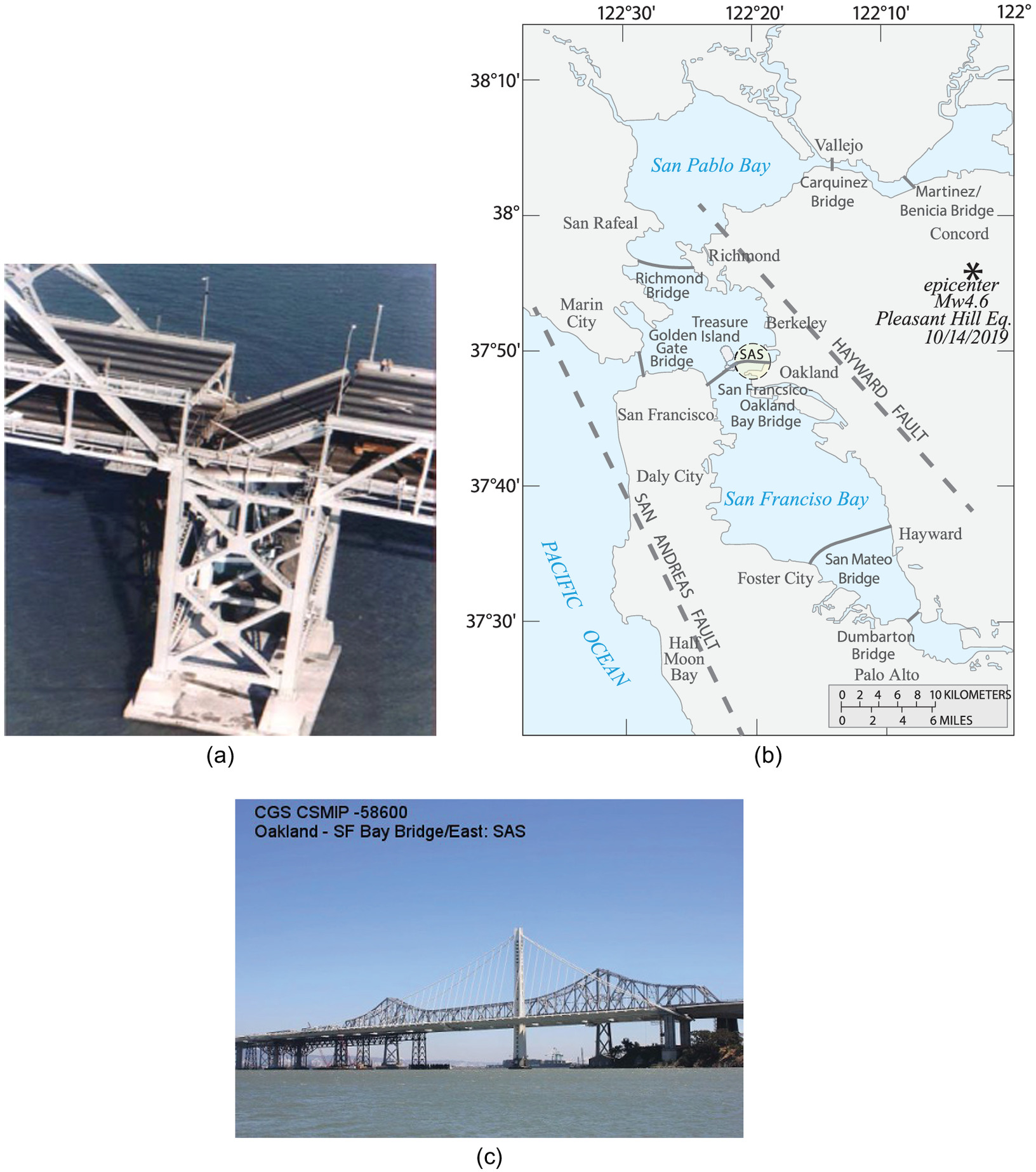
Although the damaged bridge segment was rapidly repaired, studies indicated that the old truss bridge was seismically vulnerable (Penzien et al. 2003). Hence, 24 years after LPE, in 2013, a new bridge to replace the old truss bridge was opened to service. The old truss bridge was razed. The new structure is named the Self-Anchored Suspension (SAS) Bridge. Fig. 1(c) shows a picture of both the SAS and the old truss bridge.
The SFOBB system is seismically monitored by the California Strong Motion Instrumentation Program (CSMIP) of the California Geological Survey (CGS), according to an agreement with the California Department of Transportation (Caltrans). The specific seismic monitoring array of the SAS has been assigned CSMIP station number 58600 at coordinates 37.8152° N, 122.3589° W. The SAS seismic instrumentation comprises accelerometers, tiltmeters, and displacement sensors.
While the main seismic sources affecting SAS and the whole area are known to be San Andreas and Hayward Faults, since the SAS went into service in 2013, in absence of recorded earthquake response data from large earthquakes caused by the major sources, in this paper, data recorded during a small event (the October 14, 2019, Pleasant Hill earthquake) that occurred at an epicentral distance of 29.9 km from the SAS are used. The epicentral location of this event relative to the SAS and the SFBA is provided in the map [Fig. 1(b)]. During the referenced 2019 event, the vast majority of accelerometers functionally recorded the response of the SAS Bridge; therefore, this is the basis for the selection of the 2019 event–related data set. Two other small events’ response data were not recorded by a significant percentage of the array.
Hence, the purpose of this paper is to study the response and behavior of the SAS Bridge during the referenced event only. The scope of the paper does not cover the details of 1989 Loma Prieta earthquake event or details of the fallen section of the old truss bridge. In-depth details of the Loma Prieta earthquake and its effects are provided in the USGS Professional Paper series. Why, in 1989, the section of the old truss bridge fell as it did is explained by Hanks and Brady (1991) using free-field strong motion data at key ground stations (because the SFOBB system was not instrumented at that time). Design details of the SAS are not covered herein either but are discussed by many others including Sun et al. (2004), Frick (2016), McDaniel et al. (2003), and Nader et al. (2014, 2002). The scope of the paper is devoted to the analyses of real-life behavior of the bridge using recorded data. The scope does not include finite element (FEM) analyses.
The SAS Structure and Foundation
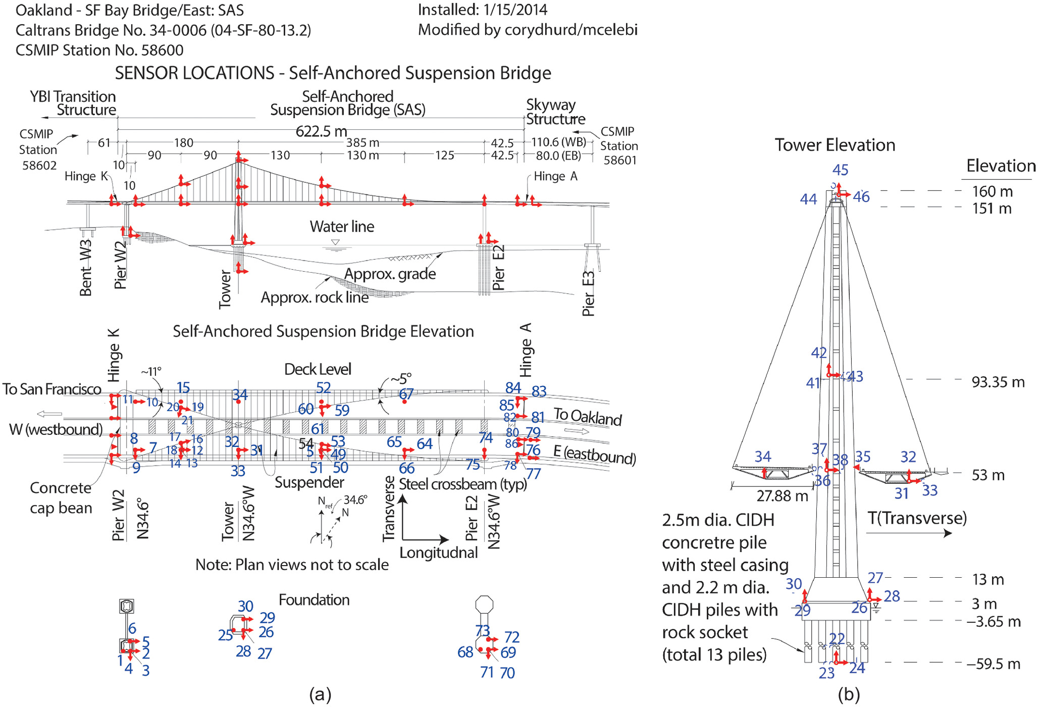
The overall SAS structural system is depicted using the schematics in Fig. 2. A concise summary of the structural system is provided in Strong Motion Center (2023). Accordingly, the SAS is the bridge structure between Pier W2 and Pier E2 (including the tower and foundations), as seen in Figs. 2(a and b), and the main deck comprises dual orthotropic steel box girders each having a width of 27.88 m (91.47 ft) The box girders are not attached to the tower. The westbound (W) and eastbound (E) girders are connected by steel crossbeams and are suspended with hangers from cables, which, in turn, are hung over a saddle system and supported at the top of a single steel tower at an elevation of 160 m (524.93 ft). The self-anchored suspension describes the cables that are anchored at Pier E2 and looped around Pier W2 through saddles (e.g., at top of the tower). In other words, there are no anchorages, as in the vast majority of suspension bridges (e.g., the two side-by-side suspension bridges between San Francisco and Yerba Buena Island, which are west of the SAS, or the Golden Gate Bridge connecting San Francisco and Northern California).
The aforementioned structural attributes are depicted in vertical and plan views in Fig. 2, which will later be reviewed for the details of the instrumentation.
It is noted herein that additional general in-plan orientations of the structure, assigned as longitudinal (L) along the length of the deck and transverse (T) perpendicular to the length of the deck, are added in the modified Fig. 2(a). These are proclaimed herein as the global coordinates of the overall SAS structure. As indicated in the figure, the total length of the deck (and therefore the SAS Bridge) is 622.5 m (2,042 ft).
The tower is a unique design [Fig. 2(b)]. There are four steel shafts that are interconnected with steel shear links. In addition, the shafts are rigidly connected at the saddle at the top of the tower, which supports and traffics the cables. The shear links are designed to experience inelastic behavior and therefore have been cyclic tested in laboratory. Detailed description of these tests are provided by McDaniel et al. (2003). The overall design of the SAS Bridge is detailed in Nader et al. (2002, 2014), and Penzien et al. (2003).
In addition, both Piers W2 and E2 comprise a concrete cap beam that is supported by concrete columns. The columns of Pier W2 are tie-downed to the foundation. The Pier E2 concrete cap beam is connected to the box girders (of the deck) with shear keys and bearings.
The foundation of the bridge is best described as such: (1) at Pier W2 as concrete footing on top of 2.5 m cast-in-drilled-hole (CIDH) concrete piles at the westbound side only; (2) at the tower as concrete footing on top of a total of 13 70-m-long piles (2.5-m-diameter concrete piles with steel casing and 2.2-m-diameter CIDH piles, all rock socketed at an elevation of ); (3) at Pier E2 as each footing cap (below the westbound and eastbound decks) rests on 8 105.5-m-long, 2.5-m-diameter cast-in-steel-shell (CISS) piles; (4) the W and E footing caps are connected by a 5.7-m-deep concrete beam; and (5) all piles are socketed to rock.
The vertical elevation in Fig. 2(b) also shows an approximate rock line and an approximate grade. The rock is described as sedimentary and what is above it as alluvium (Strong Motion Center 2023). Nader et al. (2014) describe the rock as Franciscan Formation, and the alluvium, comprising sandy clays and sand, as Alameda Formation.
Seismic Hazard and Performance Criteria
Details of seismic hazard evaluations of SAS are best described in Nader et al. (2002, 2014). In summary, a safety evaluation earthquake (SEE) and a functional evaluation earthquake (FEE) have been defined. They report that the SEE was defined by a probabilistic seismic hazard analysis with a 1,500-year return period. Design for a functional evaluation earthquake is expected to result in the SAS providing immediate full service with essentially elastic performance (but with minimal damage or minor inelastic response). On the other hand, with a SEE design, the SAS is expected to be functional even after it sustains repairable damage that can be repaired within a few days. Further details are found in Nader et al. (2002, 2014). However, the zero-period accelerations (ZPA) for the design events have not been identified in these references.
Nader et al. (2002) further report that (1) the design of the SAS is governed by the SEE, and (2) the analyses using this criterion computed longitudinal, transverse, and vertical fundamental periods (frequencies) of the SAS as 3.80 s (0.263 Hz), 3.64 s (2.75 Hz) and 4.50 s (0.222 Hz).
It is important to restate that in this paper, recorded data from sensors deployed at components of the SAS are used. Therefore, the fundamental periods (frequencies) reported by Nader et al. (2002) in the global longitudinal, transverse, and vertical coordinates of the bridge are not comparable with those dynamic response characteristics identified using the data from the small 2019 earthquake.
Seismic Instrumentation Array and Recorded Earthquake Data
Fig. 2, modified from the originals in Strong Motion Center (2023) depicts locations and orientations of most of the seismic monitoring sensors (accelerometers, tiltmeters, and displacement sensors), the north (N) and reference north (Nref) as well as the orientations of global coordinates (L and T). For ease in following the analyses of records from the many sensors, Table 1 provides the locations, orientations, and sensor types. It is noted herein that the data from tilt sensors and displacement sensors are not available. Horizontal cable sensors are oriented according to cable-specific longitudinal and translational orientations C1L and C1T for the side span and C2L and C2T for the main span. It is noted that Channels 2 and 3 malfunctioned and Channels 56, 57, and 58 were not active.
| Location | Accelerometer channels | Other sensorsa | ||
|---|---|---|---|---|
| L | T | UP | ||
| Tower top (saddle) | 44 | 46 | 45 | 47,48 (TS) |
| Tower el. 93.35 m | 41 | 43 | 42 | 39,40 (TS) |
| Tower el. 53 m (deck level) | 36 | 38 | 37 | 62,63 (TS), 5 (DS) |
| Tower el. 3 m | 26,29 | 28 | 27,30 | — |
| Tower el. = 59.5 m | 23 | 24 | 22 | — |
| Westbound (W) cable | 19 (C1L) | 21 (C1T) | 20 | — |
| Eastbound (E) cable | 16 (C1L) | 18 (C1T) | 17 | — |
| (W) Deck | — | — | 15 | — |
| (E) Deck | 12 | 14 | 13 | — |
| Pier W2 | ||||
| (W) Deck level | 10 | — | 11 | — |
| (E) Deck level | 7 | 9 | 8 | |
| (E) El. 4.18 m | 5,2 | 4 | 1,3,6 | 2,3 malfunction |
| (W) Deck at tower | — | — | 34 | — |
| (E) Deck at tower | 31 | 33 | 32 | 35 (DS) |
| 1/3 Between tower and Pier E2 | ||||
| (W) Cable el. 93.35 m | 59 (C2L) | 61 (C2T) | 60 | — |
| (E) Cable | 53 (C2L) | 55 (C2T) | 54 | — |
| (W) Deck | — | — | 52 | — |
| (E) Deck | 49 | 51 | 50 | — |
| 2/3 Between tower and Pier E2 | ||||
| (W) Deck level | — | — | 67 | — |
| (E) Deck level | 64 | 66 | 65 | — |
| (E) Pier E2 deck level | — | 75 | 74 | — |
| (E) Top of piles at Pier E2 | 69, 72 | 71 | 68,70,73 | — |
| (W) Hinge A deck level | 81,83 | 85 | 82, 84 | — |
| (E) Hinge A deck level | 76, 79 | 78 | 77,80 | 86 (DS) |
Note: L = longitudinal; T = transverse; UP = vertical; TS = tilt sensor; and DS = displacement sensor; for the side span cable orientation () is w.r.t the longitudinal axis of the side span [cable longitudinal (C1L), cable transverse (C1T)]; and for the main span [cable longitudinal (C2L), cable transverse (C2T)].
a
Data for other sensors are not available; data for Channels 56, 57, 58 are not available.
The one event during which the vast majority of accelerometers recorded the response of the SAS Bridge is the October 14, 2019, Pleasant Hill earthquake [ pacific daylight time (PDT), coordinates 37.9380° N and 122.0570° W, and 14.0 km depth that occurred at an epicentral distance of 29.9 km from the SAS, whose coordinates are 37.8152° N and 122.3589° W] (Strong Motion Center 2023). Table 1 summarizes the channel numbering system according to location and orientation.
It is important to note herein that the recorded response data served by CSMIP via Strong Motion Center (2023) are both (1) raw (unprocessed accelerations); and (2) processed [acceleration (a), velocity (v), and displacement (d)] versions. Processing is executed by CSMIP. Details of processing filters are always included in the headers of each avd data for each channel. In this study, only processed a, v, and d data sets are used as imported Strong Motion Center (2023). Further discussion of data processing is outside the scope of this study.
Analyses of Recorded Data
Acceleration Time Histories at Tops of Foundation Footing, Tower, and Downhole
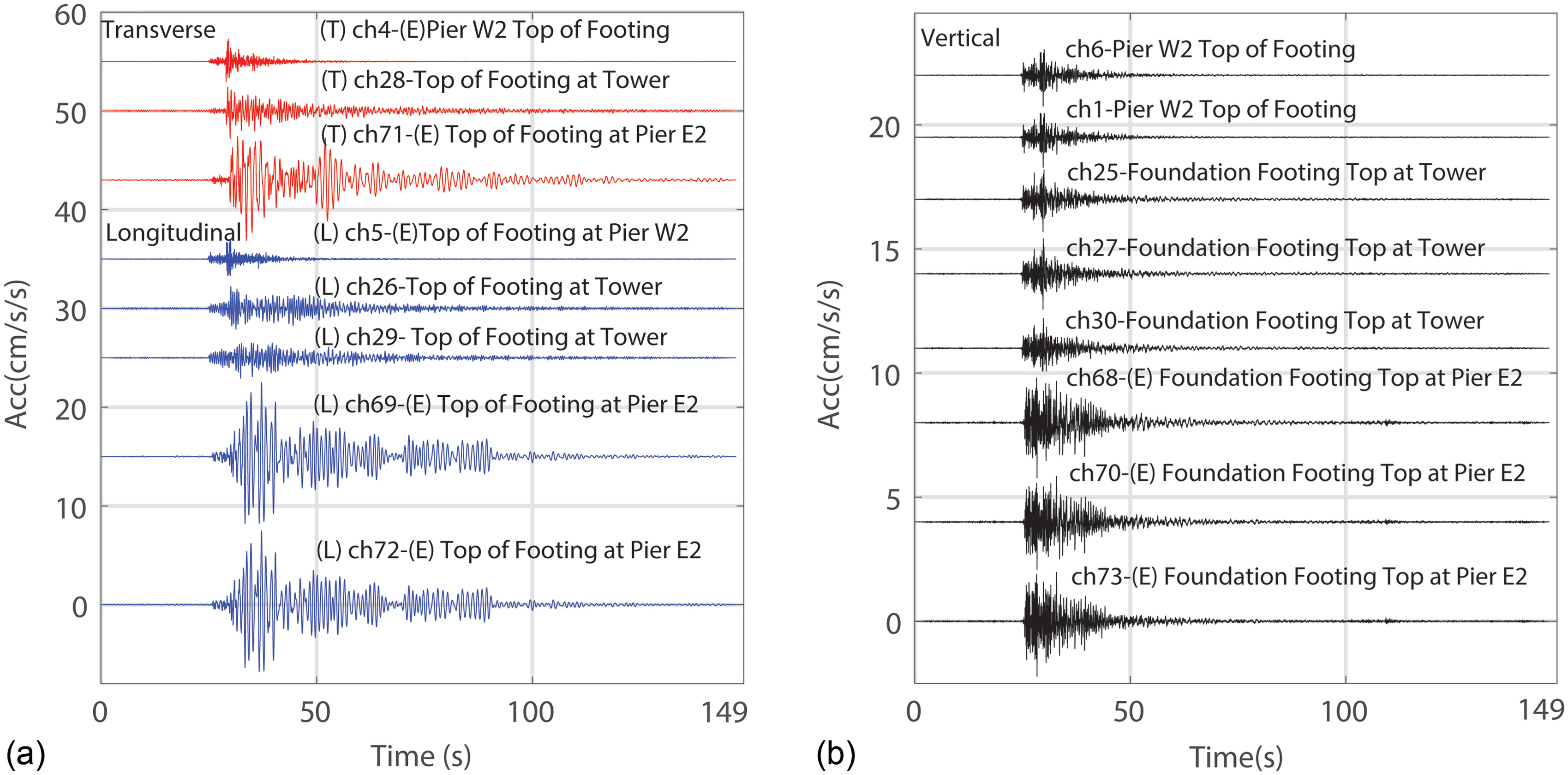
Fig. 3 shows equiscaled plots of acceleration time histories for all horizontal and vertical channels at the top locations of footings at Piers W2 and E2, as well as at the tower location. They are considered the horizontal and vertical input excitation of the SAS structural system supported by the tops of foundation footings. It is not surprising that the amplitudes of accelerations (longitudinal, transverse, and vertical) are greater for those footing top locations that are in deeper alluvial geotechnical media (Pier E2 and the tower location) as compared to those at Pier W2, which is on rock (Channels 4, 5, and 6). Also, the strong shaking duration of the Pier W2 channels (4, 5, and 6) are visually smaller in their respective orientations than those of Pier E2 and the tower location. Simply stated and as expected, motions at the rock location are amplified at alluvium locations.
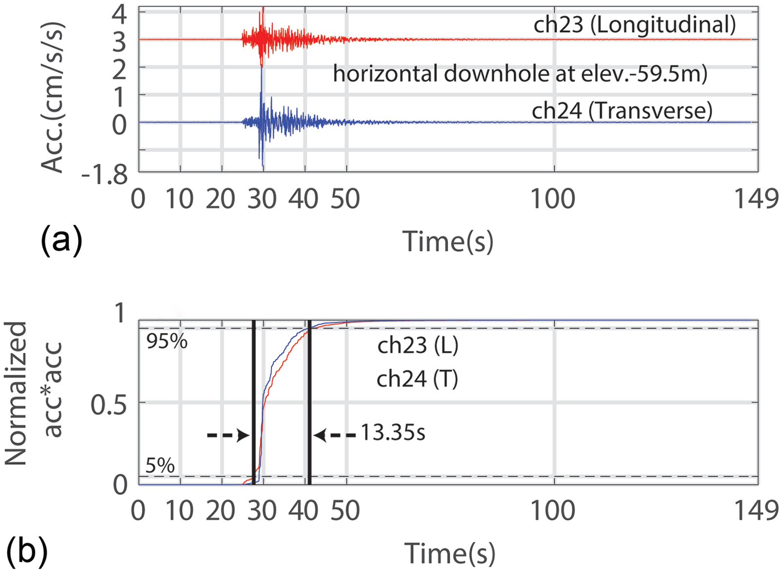
However, to compute the strong shaking duration of input horizontal motions, the recorded accelerations (recorded by Channels 23 and 24) at the borehole bottom (rock at elevation is 59.5 m) are used. Fig. 4(a) is developed to display acceleration time history plots of horizontal downhole data (of Channels 23 and 24). Fig. 4(b) shows the assessment of strong ground shaking duration a using summed squared horizontal accelerations method (Trifunac and Brady 1975; Boore and Thompson 2014). The 5%–95% method is used to define the strong shaking duration as applied in the figure in which both horizontal longitudinal and transverse Channels 23 and 24 at the borehole bottom indicate 13.25 s as an estimate of the duration of strong shaking input motions to the SAS. Later in the paper, this figure is referred to in discussions of the elongated duration of shaking at the superstructure of the SAS.
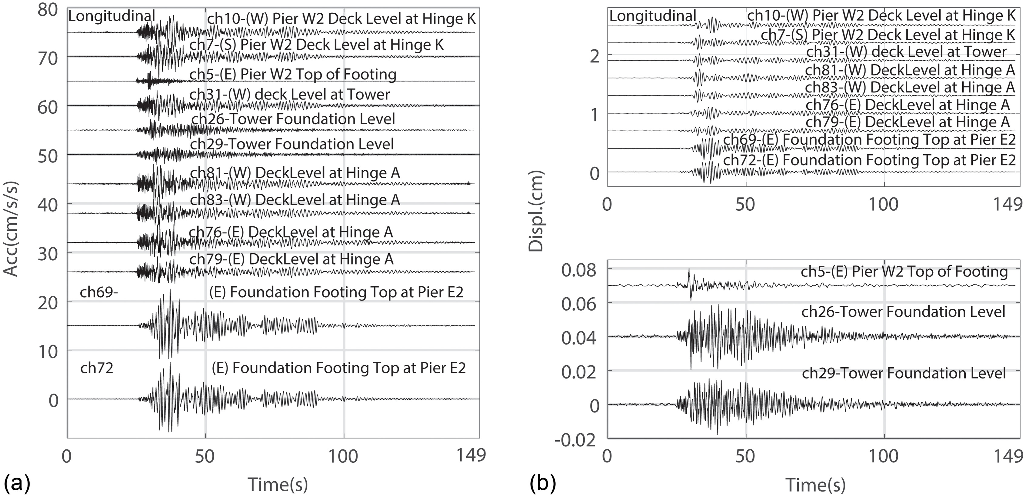
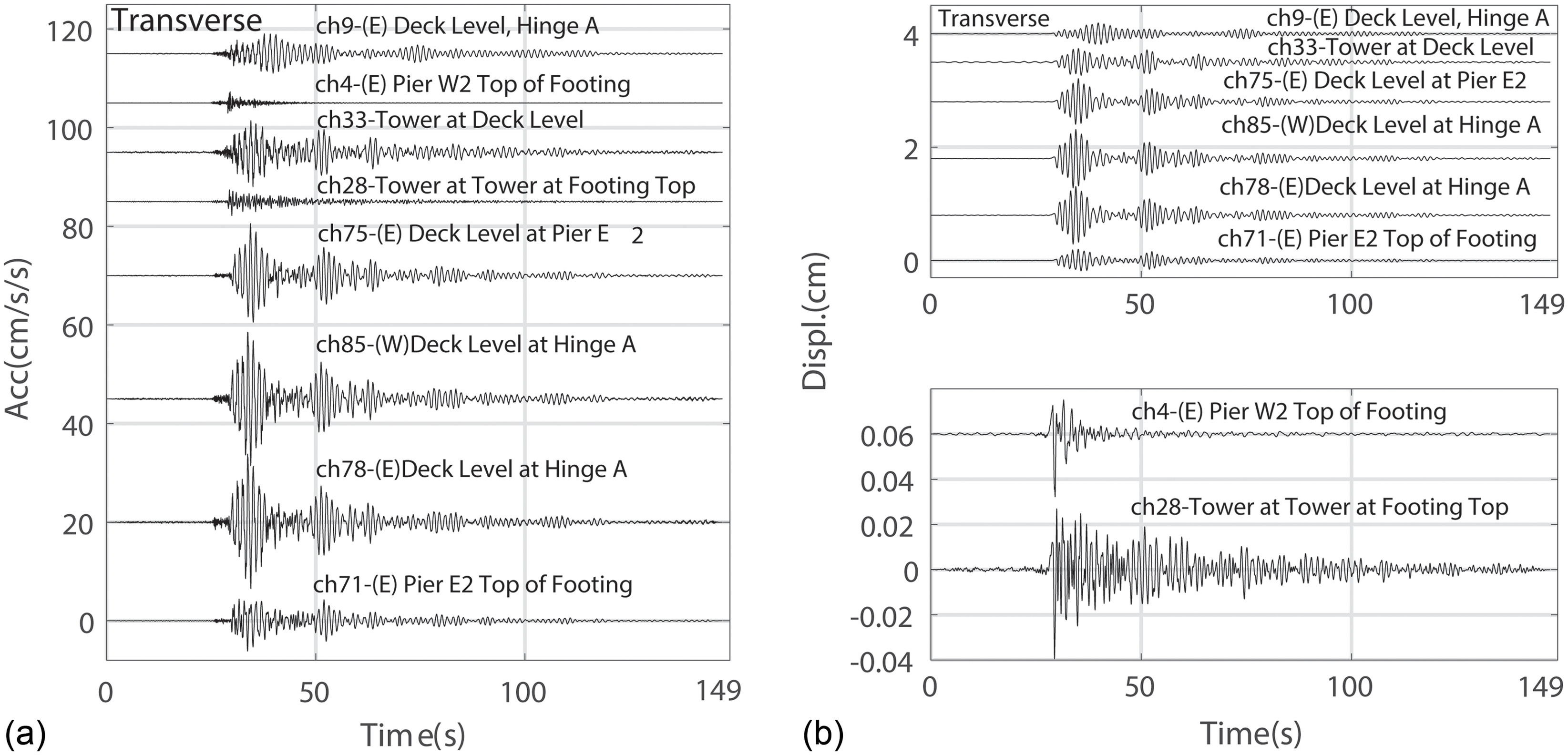
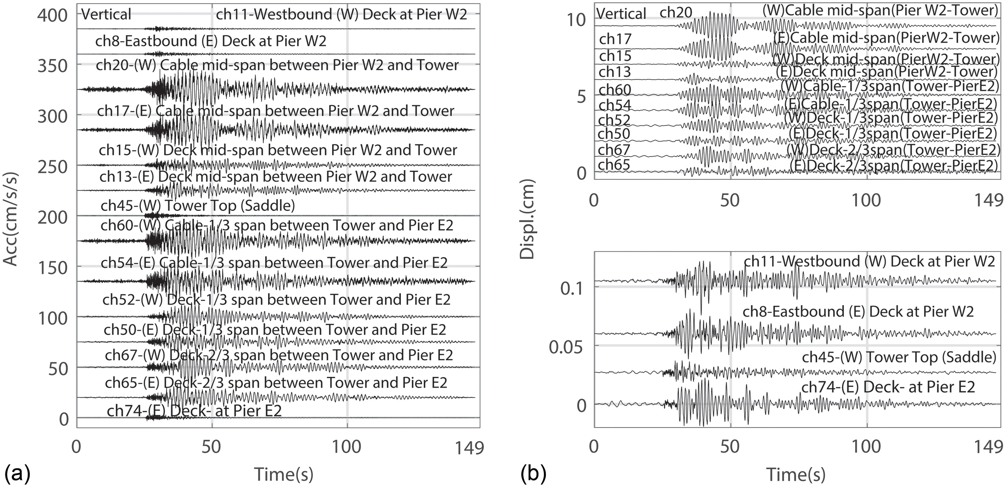
Acceleration and Displacement Time Histories at SAS Superstructure (Deck, Tower, and Cables) and Foundation Tops
For all structural histories, the figures display the strong shaking duration which, as expected, is longer than that of the input motion strong shaking duration. And, as discussed earlier and displayed in Figs. 4(a and b), particularly in the displacement time histories of numerous channels (Figs. 5–7), there is strong evidence of a repetitious beating effect that will be discussed in detail later in the paper.
Identification of Structural Dynamic Characteristics
Upfront and at the expense of being repetitious, it is important to note that sensors are deployed at the three main structural components of SAS (deck, tower, and cables) along with the foundation. Therefore, the frequencies identified from the data set will belong to the structural component and not the overall SAS with the global coordinate system.
Amplitude Spectra and Spectral Ratios (Longitudinal, Transverse, and Vertical)
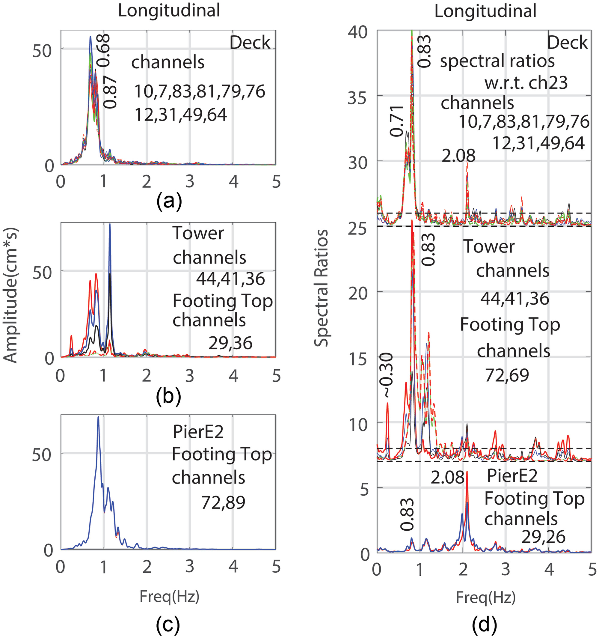
First, amplitude spectra of longitudinal, transverse, and vertical accelerations recorded by the channels of accelerometers (Table 1) are computed. Second, spectral ratios of the amplitude spectra of accelerations are computed. Longitudinal spectral ratios are computed with respect to (w.r.t) channel (ch)23 (the longitudinal downhole channel at elevation at rock). Similarly, transverse spectral ratios are computed w.r.t ch24 (the transverse downhole channel) and vertical spectral ratios are computed w.r.t ch22 (the vertical downhole channel). However, using acceleration data did not yield the expected low frequency () amplitudes in the spectra or the ratios. Therefore, in this paper, only the amplitude spectra of displacements and their spectral ratios are presented.
In Fig. 8, both the amplitude spectra [Figs. 8(a–c)] of longitudinal displacements and the spectral ratios in Fig. 8(d) (with respect to the amplitude spectrum of downhole ch23) allow identification by peak picking of the lowest frequency at and others at 0.71, 0.83, and 2.08 Hz. This first modal frequency at is clear only in these plots of spectral ratios of amplitude spectra of displacements and not in those computed from accelerations. The frequency at 0.71 Hz most likely appears due to coupling with modes other than longitudinal. It is also noted that both the amplitude spectra and spectral ratios are repeatable for all channels in each frame.
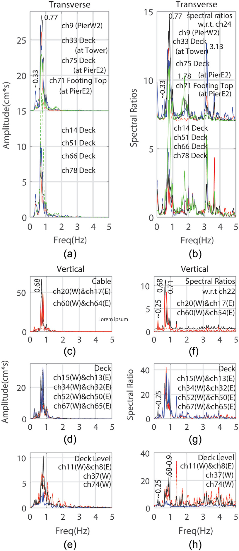
In Fig. 9(a) computed amplitude spectra of transverse displacements and (b) their spectral ratios that ents allow the identification of frequencies as , 0.77, 1.78, and 3.13 Hz. Again, both the amplitude spectra and spectral ratios are repeatable for all channels. Similarly, in Figs. 9(c–e), computed amplitude spectra of vertical displacements of deck and cable locations, and Figs. 9(f–h), spectral ratios of the amplitude spectra, allow the identification of frequencies at and .
Displacement Time Histories and Amplitude Spectra for Cables
Vertical acceleration and displacement time histories of cable channels (20,17, 60, and 54) are plotted in Fig. 10. Their amplitude spectra are included and are consistent with the amplitude spectral and spectral ratio peak for the first mode at for the deck (Fig. 10). This is not surprising because cables are connected to the deck with hangers, which ensures that in the vertical direction, cable and deck motions have to be compatible both in amplitude and frequency.

In Figs. 10(a–c), time histories of previously discussed cable-specific oriented horizontal [longitudinal (CL) and transverse (CT)] displacements are plotted. C1L and C1T refer to the 180-m-long (590.55-ft) side span cable, and C2L and C2T refer to the 385-m (1,261.10-ft) main span cable [Fig. 10(a)]. Orientation angles of the cables w.r.t the longitudinal axis of the bridge are shown in Fig. 2(a). Fig. 10(a) displays that the amplitudes of longitudinal displacements (C1L and C2L) are comparable in amplitudes and are therefore plotted in one frame. Hence, in Fig. 10(d), it follows that their amplitude spectra also have comparable amplitudes to fit within the plotting frame but have peaks at slightly different frequencies ( and 0.8 Hz).
On the other hand, the amplitudes of cable transverse displacement time histories for C1T (side span) and C2T (main span) are significantly () different. Hence, Fig. 10(b) hosts the C1T time histories and Fig. 10(c) hosts the C2T time histories. Therefore, it follows that amplitude spectra of transverse displacements C1T and C2T are plotted separately in Figs. 10(e and f), respectively.
In the time history plots [Figs. 10(a and b)], repetitious beating is observed and the corresponding amplitude spectra have distinct spectral peaks. The same is not repeated for the cable transverse time histories [Fig. 10(c)] of the main span (C2T) locations, as defined by the displacement time histories of Channels 61 and 55. Consequently, amplitude spectra of displacement of Channels 61 and 55 display multiple peaks within the 0–2 Hz frequency band. This may be interpreted to be due to the longer lengths of main span cables and the interaction of the same with the tower and deck. The frequencies identified by peak picking are summarized in Fig. 14 later in the paper. The beating effect is discussed in more detail in a separate section also later in the paper.
System Identification and First Modal Shapes
Subspace State Space System Identification (N4SID), coded in Matlab (Mathworks 2020), is used to identify modal shapes, frequencies (f), and critical damping percentages (). Background information for N4SID is provided in Van Overschee and De Moor (1994) and Ljung (1999) and are not repeated herein. Displacement data was used for N4SID computation. However, using all available data in all orientations could not be used in one execution of N4SID because of the large size of the number of equations to be solved. Hence, N4SID is applied using several orientations and structural-component-specific displacement subset data to successfully estimate the prestated modal shapes, frequencies (f), and critical damping percentages ().
In Fig. 11(a), the extracted first translational and vertical mode shapes for only the deck are shown. The identified transverse first mode frequency (period), is 0.36 Hz (2.79 s), and the critical damping percentage is 2.11%, both of which are provided in the figure. The identified vertical first mode frequency (period), , is 0.24 Hz (4.14 s), and the critical damping percentage is 2.64%, both of which are provided in the figure. It is noted that the deck first mode shapes in the vertical direction for the side span and main span are in the opposite sense vertically. This is expected for this bridge because there is no physical restraint of the deck at the tower location; however, the hanger-cable-tower pull action for the main span forces the side span to displace in the opposite sense vertically. There is no other explanation.

Similarly, in Fig. 11(b), the extracted first longitudinal and transverse mode shapes for the tower only are shown. The identified longitudinal first mode frequency (period) is 0.47 Hz (2.14 s) and the critical damping percentage is 3.14%, both of which are provided in the figure. The identified transverse first mode frequency (period) is 0.36 Hz (2.79 s) and the critical damping percentage is 4.83%, both of which are provided in the figure.
It is noted that the frequencies limited to the first mode as identified by N4SID method compare well with those identified by peak picking using spectral ratios. On the other hand, the damping percentages computed by the N4SID method are difficult to confirm except for that by the well-known logarithmic decrement method (Chopra 2001). An example using the logarithmic decrement method is provided later in the paper. All identified dynamic characteristics (frequencies and damping) are summarized in Fig. 14 later in the paper.
Beating Effect
Beating effects have been observed in response data of many buildings and have been studied in depth by Boroschek and Mahin (1991) resulting in a formula for computing beating periods of buildings when torsional and translational natural periods of vibration are close (or closely coupled)where and = translational and torsional periods, respectively; = beating period; and = beating frequency. The beating period () is twice the inverse of beating frequency () (). Beating effect is mainly observed when the damping in the structural system is small. It occurs when repetitively stored potential energy, produced during coupled translational and torsional deformations, turns into repetitive vibrational energy.
(1)
To the best knowledge of the author, there are only a few publications that refer to beating effects of long-span bridges that are discussed or studied using earthquake response data. The presence of beating effects are observed in the earthquake response data recorded by the seismic monitoring array of the Cape Girardeau, Missouri, bridge (Çelebi 2006a) and the Carquinez, California, suspension bridge data set, recorded during the South Napa earthquake of August 24, 2014 (Çelebi et al. 2019). However, in the Golden Gate Bridge earthquake response study using data from three different events, a beating effect was not observed (Çelebi 2012). In addition, within the last three decades, including the study by Boroschek and Mahin (1991), there are a limited number of studies related to some tall buildings experiencing beating phenomena, as observed from recorded earthquake response data, including: (1) a 13-story building during the 1989 Loma Prieta, California, earthquake (Çelebi and Liu 1998); (2) the 20-story Atwood Building in Anchorage, Alaska, during the Tazlina Glacier earthquake in April 2005, along with other earthquakes (Çelebi 2006b); (3) the tallest California building, the 73-story Wilshire Grand of Los Angeles, during the Ridgecrest, California, earthquake of July 5, 2019 (Çelebi et al. 2020); and (4) the 61-story (the tallest building in San Francisco) Salesforce Tower during the January 4, 2018, Berkeley earthquake (Çelebi et al. 2019). A detailed study to quantify the effect of beating in lengthening the vibrational duration, and therefore the vibrational energy, of tall buildings is presented in a recent paper (Çelebi 2018). Finally, it should be stated that the subject of beating behavior induced by seismic or strong winds is, unfortunately, not included in structural dynamic textbooks either.
Why beating is important is displayed in Figs. 12(a and b), in which several cycles of beating in extends the duration of strong shaking in the translational (ch51) and vertical accelerations (ch50) at the location of the main span of the deck. As done in Fig. 4, 5%–95% normalized summed squared acceleration method (Trifunac and Brady 1975) yields the estimated structural strong shaking duration as and significantly longer than the for the ground motion (Fig. 4). Hence, (1) it is therefore deduced that going from to implies an elongation of strong shaking duration of the structure, at least for a significant percentage of the length of the time difference between 60 and 13.25 s; and (2) the additional step-like vibrational energy (as represented by the normalized summed squared acceleration) is added several times, and on a regular and repetitious basis, due to beating. Note that the observed length of each beating cycle time (or beating period) differs for the vertical as compared to transverse acceleration time history; both, however, exhibit the steps in normalized energy as represented by the normalized summed square of acceleration. From this plot (Fig. 12), the beating periods in the translational and vertical direction of the main span deck are extracted to be and , respectively. As a result, the repetitious exchange between vibrational and potential energy that causes the elongated response may result in low-cycle fatigue of the elements of the suspension bridge (e.g., the cables, hangers, deck and tower). It is important to mention that the data record length is important when computing summed squared acceleration time history. The reason for this is that the record length of 149 s in the data set used in this study is based on a preset start recording trigger and an end recording acceleration threshold (as opposed to continuous recording and selecting the record length on demand). This means that it is likely that the beating continues beyond the stop recording threshold (149 s in this case), possibly elongating the shaking even more than the estimated . Finally, it was stated earlier that important requisite conditions for beating effects to materialize are a low critical damping percentage of the structure and its components (tower, deck, and cables) and closely coupled modes.
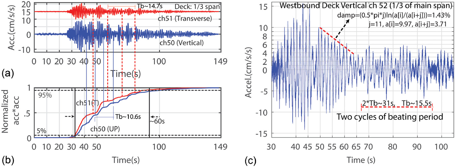
The computed critical damping percentages of components using the N4SID system identification method are all (varying between 2.11% and 4.83%). Another way to assess the low critical damping percentage is by the well-known textbook logarithmic decrement method (Chopra 2001) as demonstrated in Fig. 12(c), which results in 1.43% damping and which easily allows for the identification of the repetitious beating period as 15.5 s. The low-amplitude shaking data set used in this study implies only elastic response.
About Apparent Frequency
The fact that frequencies and critical damping percentages are identified for the components (tower, deck, and cables) of the SAS does not allow for direct comparison with those characteristics as computed for the total SAS structural system in its global coordinates (as has been done by Nader et al. 2002). Hence, an exploration of making use of an apparent frequency computation is appropriate to estimate global coordinate–based frequencies for the SAS, using those identified for the components (tower, deck, and cables). This is being attempted even though the frequencies of the components are identified from low-amplitude shaking data. The Nader et al. (2002) frequencies (periods) are computed for the much larger–amplitude SEE event, and for longitudinal, transverse, and vertical orientations of the SAS, respectively, as 0.263 Hz (3.80 s), 2.75 Hz (3.64 s), and 0.222 Hz (4.50 s).
The apparent frequency () approach is widely known and used in soil-structure analyses of buildings as: where and are the frequencies of the structure and soil, respectively (Jacobsen and Ayre 1958; Luco et al. 1986; Trifunac et al. 2001). This relationship is described by Trifunac et al. (2001) as a combination rule whereby apparent frequency, , (period, ) is shorter (longer) than the shortest frequencies (longest periods) of interacting parts.
From the aforementioned relationship, the apparent frequency () and period () are computed directly as
(2)
However, in the experience from the Golden Gate Bridge study (Çelebi 2012), as also may be applicable for the majority of long-span suspension bridges, when, for example, only the deck () and tower () are considered, and when the difference between them is large enough, the apparent frequency is identical to the lower of the two, which always is that of the deck. For the Golden Gate Bridge, the apparent frequency () of 0.13 Hz was computed from the interacting tower’s longitudinal () and the deck’s vertical (0.13 Hz) motions, and is the same as the deck’s vertical motion (0.13 Hz) [as computed by ].
Similarly, in the case of the Carquinez Suspension Bridge study (Çelebi et al. 2019), the tower longitudinal frequency (0.39 Hz) is significantly higher than that of the deck vertical frequency (0.17 Hz). The resulting apparent frequency, (at ) is very close to (at 0.17 Hz).
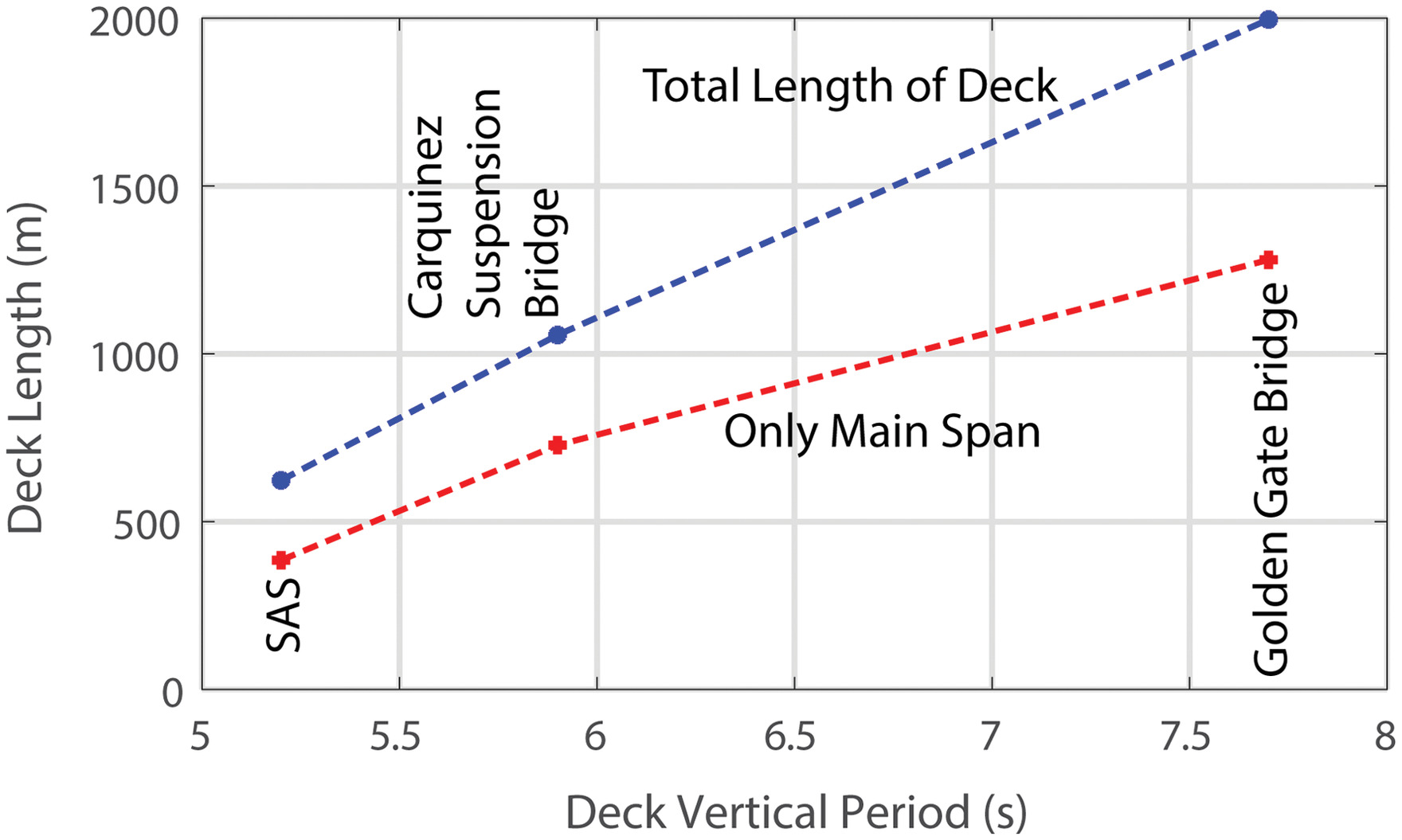
Applying Eq. (2) to the SAS and using deck vertical frequency (period) as 0.25 Hz (4.0 s), and tower longitudinal frequency (period) as 0.3 Hz (3.33 s), apparent frequency (period) () is obtained as 0.19 Hz (5.20 s). Similarly, using tower longitudinal frequency (period) as 0.3 Hz (3.33 s), and tower transverse frequency (period) as 0.33 Hz (3.0 s), apparent frequency (period) () is obtained as 0.22 Hz (4.48 s). Table 2 summarizes the apparent frequencies for these three bridges (the SAS, Golden Gate, and Carquinez). Fig. 13 displays the variation of apparent periods against both the main span only and the total length of the deck. There is surprisingly almost a linear variation even though the SAS has only one tower and one side span. Naturally, more empirical data is required to make a claim of reliable correlation.
| Bridge | Deck length (m/ft) | Tower height above (m/ft) | Deck (UP) apparent T/f (s/Hz) | ||
|---|---|---|---|---|---|
| Main span | Total | Deck level | Footing level | ||
| SAS (this study) | |||||
| Golden Gate (Çelebi 2012) | |||||
| Carquinez (Çelebi et al. 2019) | |||||
Summary, Discussions, and Conclusions
Data from dozens of sensors of the SAS’s seismic monitoring array deployed at its components (tower, deck, and cables) recorded during the low-amplitude shaking caused by the October 14, 2019, Pleasant Hill earthquake are used in this study. This set of data is selected as, to date, the one (of three) with the largest number of sensors that successfully recorded the event. Global structural coordinates (longitudinal, transverse, and vertical coordinates) defined for the overall SAS structure are also coordinates for the three main SAS components (tower, deck, and cables). It is important to note and repeat that the sensors are deployed at select locations of the components. Hence, the identified structural dynamic characteristics (frequencies and critical damping percentages) from channel-based data are affiliated with the particular components at which the sensors have been deployed, and, essentially not the global SAS structure. The various spectral plots (many of which have several sensors on the same component) presented in this paper indicate dominant modal frequencies as belonging to each component. Therefore, it is not possible to make a direct declaration of the dynamic characteristics for the overall SAS structure. All the identified fundamental frequencies (periods) and critical damping percentages of components of the SAS (tower, deck, and cables) in the global coordinates (longitudinal, transverse, and vertical directions) are summarized in Fig. 14.
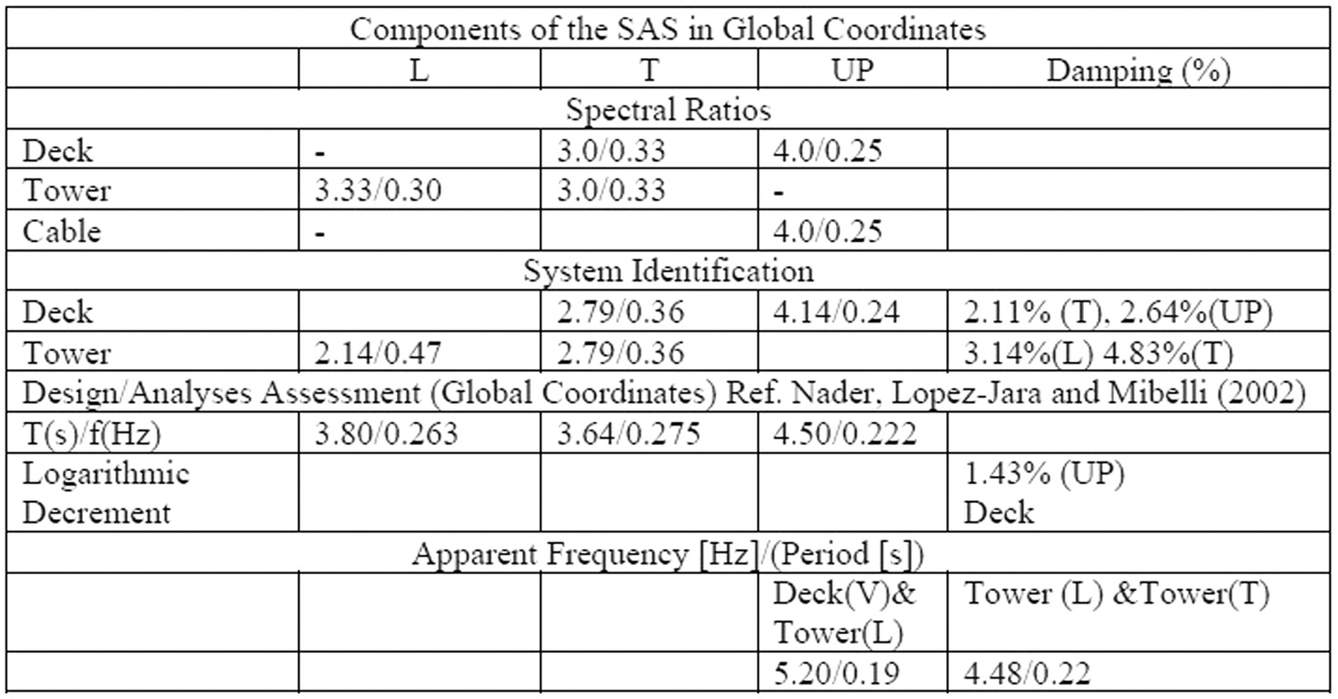
On the other hand, only three fundamental periods (frequencies) [3.80 s (0.263 Hz), 3.64 s (0.275 Hz), and 4.50 s (0.222 Hz)] in the global (longitudinal, transverse, and vertical) coordinates for the overall SAS structure are publicly available, as reported by Nader et al. (2002), as a result of mathematical model analyses for the much larger input motions defined by the SEE. For general comparison, these fundamental frequencies (periods) are also included in Fig. 14.
Hence, there are two issues: (1) the low-amplitude data used to identify dynamic structural characteristics for the components, and (2) the much larger SEE criteria–based, mathematical analysis–based results for fundamental modal periods (frequencies) only. Therefore, it is not valid to directly compare the dynamic response characteristics identified in this study (using low-amplitude shaking earthquake data) with those from the design-level SEE earthquake. Nonetheless, to make sense of the data-based identified data, a couple of apparent periods (frequencies) have been computed (and are included in Fig. 14) to be representative of the overall global structure. It is noted that the computed apparent period for vertical direction (5.20 s) is larger than the 4.50 s value obtained from the reported SEE analysis. The deduction, then, is that for a much larger strong shaking event, the apparent period will be even longer. Therefore, this may infer a level of discrepancy between data-based values and mathematical model–based SEE analysis values. Future analyses of recorded data from stronger shaking events could be useful to answer this issue better.
N4SID system identification computations resulted in low critical damping percentages (), all less that the usual 5% used in practice. An additional low critical damping percentage (1.43%) has been identified by logarithmic decrement method.
Closely coupled modes and low critical damping percentages lead to responses with a significant beating effect for which beating periods have been computed to be approximately 12–15 s. This behavior is observed in all acceleration and displacement time histories of the three structural components (tower, deck, and cables). It is recommended that in order to attenuate the effect of beating, some additional manufactured dampers may be added to the cables and, if necessary, to the deck and tower.
It is desirable to collect more data from SAS-type bridges (if others exist) and from conventional suspension bridges (with two towers and anchorages at two ends of the deck) to advance correlation of deck lengths with the fundamental vertical period of the decks, and therefore, the bridges. Such a relationship could prove to be useful as a rule of thumb estimation option of vertical fundamental periods (frequencies) of long-span suspension bridges.
Data Availability Statement
Some or all data, models, or code that support the findings of this study are available from the corresponding author upon reasonable request. Actual time histories of all recorded data used in this paper are freely available at www.strongmotioncenter.org. At this site, select structural data and enter station code: 58600 for SAS. It is important to note herein that the recorded response data served by CSMIP via www.strongmotioncenter.org are both (1) raw (unprocessed accelerations), and (2) processed [acceleration (a), velocity (v), and displacement (d)] versions. Processing is executed by CSMIP. Details of processing filters are always included in the headers of each avd data for each channel. In this study, only processed a, v, and d data sets are used as imported from www.strongmotioncenter.org.
Acknowledgments
Cory Hurd of USGS helped with developing Fig. 1(b) and modifying Figs. 2 and 3. Ms. C. E. Ashcroft of USGS carefully grammatically edited the draft. Thanks are due to Grace Parker and Robert Chase, both from USGS, for reviewing earlier drafts of the paper. Any use of trade, firm, or product names is for descriptive purposes only and does not imply endorsement by the US Government.
References
Boore, D. M., and E. M. Thompson. 2014. “Path durations for use in the stochastic-method simulation of ground motions.” Bull. Seismol. Soc. Am. 104 (5): 2541–2552. https://doi.org/10.1785/0120140058.
Boroschek, R. L., and S. A. Mahin. 1991. Investigation of the seismic response of a lightly-damped torsionally-coupled building. Berkeley, CA: Univ. of California.
Çelebi, M. 2006a. “Real-time seismic monitoring of the new Cape Girardeau Bridge and preliminary analyses of recorded data: An overview.” Earthquake Spectra 22 (3): 609–630. https://doi.org/10.1193/1.2219107.
Çelebi, M. 2006b. “Recorded earthquake responses from the integrated seismic monitoring network of the Atwood building, Anchorage, Alaska.” Earthquake Spectra 22 (4): 847–864. https://doi.org/10.1193/1.2359702.
Çelebi, M. 2012. “Golden gate bridge response: A study with low-amplitude data from three earthquakes.” Earthquake Spectra 28 (2): 487–510. https://doi.org/10.1193/1.4000018.
Çelebi, M. 2018. “Quantifying the effect of beating inferred from recorded responses of tall buildings.” In Proc., 11th National Conf. in Earthquake Engineering. Los Angeles: Earthquake Engineering Research Institute.
Çelebi, M., S. F. Ghahari, H. Haddadi, and E. Taciroglu. 2020. “Response study of the tallest California building inferred from the Mw7.1 July 5, 2019 Ridgecrest, California earthquake and ambient motions.” Earthquake Spectra 36 (3): 1096–1118. https://doi.org/10.1177/8755293020906836.
Çelebi, M., S. F. Ghahari, and E. Taciroglu. 2019. “Responses of the odd couple Carquinez, CA, suspension bridge during the Mw6.0 south Napa earthquake of August 24, 2014, 2019.” J. Civ. Struct. Health Monit. 9 (5): 719–739. https://doi.org/10.1007/s13349-019-00363-6.
Çelebi, M., and H. P. Liu. 1998. “Before and after retrofit- response of a building during ambient and earthquake motions.” J. Wind Eng. Ind. Aerodyn. 77 (8): 259–268.
Chopra, A. K. 2001. Dynamics of structures. 2nd ed. Upper Saddle River, NJ: Prentice Hall.
Frick, K. T. 2016. Remaking the San Francisco–Oakland Bay Bridge: A case of shadowboxing with nature. New York: Routledge.
Hanks, T. C., and G. A. Brady. 1991. “The Loma Prieta earthquake, ground motion and damage in Oakland and treasure Island and San Francisco.” Bull. Seismol. Soc. Am. 81 (5): 2019–2047. https://doi.org/10.1785/BSSA0810052019.
Jacobsen, L. S., and R. S. Ayre. 1958. Engineering vibrations. New York: McGraw-Hill.
Ljung, L. 1999. System identification: Theory and user. Upper Saddle River, NJ: Prentice Hall.
Luco, J. E., H. L. Wong, and M. D. Trifunac. 1986. Soil-structure interaction effects on forced vibration tests. Los Angeles: Univ. of Southern California.
Mathworks. 2020. “Matlab users guide.” In System identification toolbox for use with Matlab. South Natick, MA: The Mathworks Inc.
McDaniel, C. C., C. M. Uang, and F. Seible. 2003. “Cyclic testing of built-up steel shear links for the New Bay bridge.” J. Struct. Eng. 129 (6): 801–809. https://doi.org/10.1061/(ASCE)0733-9445(2003)129:6(801).
Nader, M., J. Duxbury, and B. Maroney. 2014. “Seismic design of the self anchored suspension San Francisco Oakland Bay bridge.” In Proc., 37th Int. Association for Bridge and Structural Engineering (IABSE) Symp. Zurich, Switzerland: International Association of Bridge and Structural Engineering.
Nader, M., J. Lopez-Jara, and C. Mibelli. 2002. “Seismic design strategy of the new San Francisco-Oakland Bay Bridge self-anchored suspension span.” In Proc., 3rd National Seismic Conf. on Bridges and Highways: Advances in Engineering and Technology for the Seismic Safety of Bridges in the New Millennium Federal Highway Administration. Sacramento: California DOT.
Penzien, J., F. Seible, B. A. Bolt, J. M. Idriss, R. F. Nicoletti, J. Preece, and J. E. Roberts. 2003. “Board, Caltrans seismic advisory.” In The race to seismic safety. Washington, DC: Department of Transportation.
Strong Motion Center. 2023. “Virtual data report for earthquakes.” Accessed October 18, 2022. http://www.strongmotioncenter.org/.
Sun, J., R. Manzanarez, and M. Nader. 2004. “Suspension cable design of the New San Francisco–Oakland Bay bridge.” J. Bridge Eng. 9 (1): 101–106. https://doi.org/10.1061/(ASCE)1084-0702(2004)9:1(101).
Trifunac, M. D., and A. G. Brady. 1975. “A study on the duration of strong earthquake ground motion.” Bull. Seismol. Soc. Am. 65 (3): 581–626.
Trifunac, M. D., S. S. Ivanovic, and M. I. Todorovska. 2001. “Apparent periods of a building: Fourier analyses.” J. Struct. Div. 127 (Apr): 517–526. https://doi.org/10.1061/(ASCE)0733-9445(2001)127:5(517).
United States General Accounting Office Report to Congressional Requesters. 1990. “Loma Pieta earthquake.” In Collapse of the Bay bridge. Washington, DC: United States General Accounting Office.
Van Overschee, P., and B. De Moor. 1994. Subspace identification for linear systems. Dordrecht, Netherlands: Kluwer Academic Publishers.
Information & Authors
Information
Published In

Journal of Structural Engineering
Volume 149 • Issue 6 • June 2023
Copyright
This work is made available under the terms of the Creative Commons Attribution 4.0 International license, https://creativecommons.org/licenses/by/4.0/.
History
Received: Jun 6, 2022
Accepted: Jan 6, 2023
Published online: Mar 31, 2023
Published in print: Jun 1, 2023
Discussion open until: Aug 31, 2023
ASCE Technical Topics:
- Bays
- Bridge decks
- Bridge engineering
- Bridge towers
- Bridges
- Bridges (by type)
- Cable stayed bridges
- Cables
- Coastal engineering
- Coasts, oceans, ports, and waterways engineering
- Decks
- Earthquakes
- Engineering fundamentals
- Equipment and machinery
- Geohazards
- Geotechnical engineering
- Structural engineering
- Structural systems
- Structures (by type)
- Suspension bridges
- Towers (by type)
- Truss bridges
Authors
Metrics & Citations
Metrics
Citations
Download citation
If you have the appropriate software installed, you can download article citation data to the citation manager of your choice. Simply select your manager software from the list below and click Download.