An Analytical Method to Reproduce Seismic Behavior of a Two-Story Cross-Laminated Timber Building at Large Deformation
Publication: Journal of Structural Engineering
Volume 149, Issue 6
Abstract
Understanding the seismic resistance mechanisms and safety limits of cross-laminated timber (CLT) buildings and performing an accurate evaluation of their seismic performance is critical in earthquake-prone areas such as Japan, the US, and Italy to ensure that human lives are protected against major earthquakes. However, the knowledge from shaking table tests of full-scale CLT buildings is limited, and most tests’ maximum interstory drift is less than 4%. As a first step toward collapse analysis, this study replicated a full-scale two-story shake table experiment with a maximum interstory drift of 8.77%. The analysis software was developed by the authors and modified to consider the restoring force and the effect to replicate seismic behavior at large deformation. The skeleton curve parameters were employed in the analysis model and then changed. The results that matched the experimental results well were searched comprehensively by performing data assimilation. As a result, both the overall behavior (story shear force–interstory drift relationship) and the detailed behavior (uplift displacement of CLT wall foot of the first story) were consistent with the experimental results, indicating that the proposed analytical method can replicate the seismic behavior of CLT buildings even at large deformation.
Introduction
Timber engineering has experienced enormous research and development due to the increased interest in sustainable construction. Cross-laminated timber (CLT) has become a well-known choice for high-rise timber buildings.
The seismic performance of CLT buildings has been investigated using monotonic and quasistatic cycle tests of full-scale CLT buildings (Zhang et al. 2021; Popovski and Garvic 2016). In 2007, the Trees and Timber Institute of the National Research Council of Italy (CNR—IVALSA), Shizuoka University, Building Research Institute, and the National Institute for Earth Science and Disaster Prevention in Japan (NIED) (Ceccotti 2008; Ceccotti et al. 2013) performed full-scale shaking table tests of three- and seven-story CLT buildings as part of the Construction System Fiemme (SOFIE) project. During the tests, no residual damage was observed after the destructive earthquakes. The maximum interstory drift of the seven-story building was 67 mm, which was 2.2% of the story height of of the second and third floors of the building during the Japan Meteorological Agency (JMA) Kobe 100%. Furthermore, a 5-story CLT building with narrowed-panel CLT was tested on a shaking table (Sato et al. 2019). During the JMA Kobe 100% test, the compressive rupture of CLT and yielding of all tensile bolts were observed, and a maximum interstory drift of 3.7% was measured on the plane on the second story. In the US, a full-scale shaking table test of a two-story CLT building with replaceable components was performed in a series of research projects on CLT buildings (Blomgren et al. 2019). Interstory drift of 4.29% during the Northridge maximum considered earthquake (MCE+) hazard level was measured. The present study reproduced a shaking table test with a maximum interstory drift of 8.77% via numerical analysis, which was 263 mm for a floor height of 3 m at JMA Kobe 140% intensity, exceeding the aforementioned values.
The numerical analysis of buildings with a CLT panel is performed using various analysis tools. The SOFIE project shake table experiments were tracked using analysis software Drain–3DX, SAP2000, and Abaqus (Ceccotti and Follesa 2006; Dujic et al. 2010; Rinaldin and Fragiacomo 2016). Furthermore, time-history analysis of multistory CLT buildings of different specifications was performed using software SAPWood to investigate the behavior factor of CLT buildings (Pei et al. 2013). The finite-element method (FEM), the basic theory used by the aforementioned analysis tools, originally was designed for stress analysis, and it is useful for analyzing a continuum but is not useful for numerical analysis in large-deformation regions in which the member becomes noncontinuous after failure.
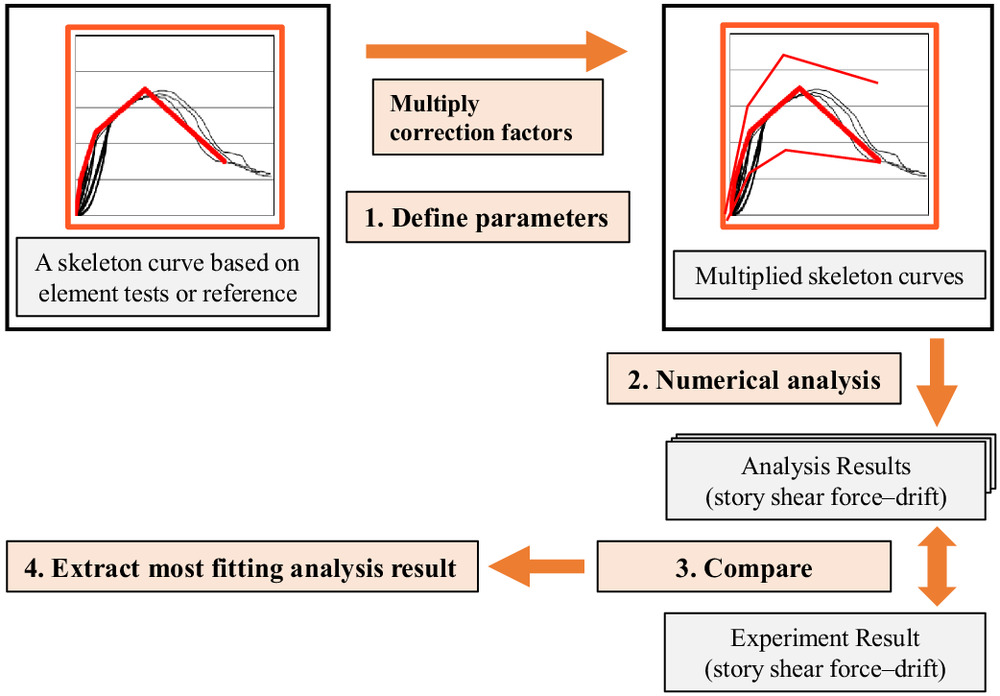
In earthquake-prone areas, such as Japan, the US, and Italy, it is critical to clarify the safety limits and collapse mechanism of CLT buildings through collapse experiments and reproductive analysis as well as to accurately evaluate the seismic performance of CLT buildings to protect human lives in the event of a massive earthquake. Consequently, the authors developed the analysis software wallstat, which is based on the extended distinct-element method (EDEM). In this study, the authors modified and developed wallstat version 5.1 for CLT buildings. Using the developed software, we tracked the test results when CLT buildings encountered considerable deformation. Elemental experiments were used to define the mechanical properties of CLTs and joints. According to Yasumura et al. (2016), the simple combinations of elemental experiments cannot reproduce full-scale experimental results accurately. An analysis called data assimilation (Namba et al. 2021) was performed. The process of data assimilation is shown in Fig. 1. First, spring and element parameters were multiplied by the correction factors to create various skeleton curves for the spring. Then the analytical and experimental results were compared in terms of only the shear force–interstory drift of the first story; finally, the analytical result with the smallest error from the experimental results was extracted. The experimental results were reproduced, and the validity of the analytical method was confirmed. Afterward, the analysis results before and after the data assimilation were compared, and the causes of the differences were discussed.
Outline of Analytical Method
Previous research widely has used numerical calculations based on FEM, as represented using the matrix method, for the time-history response analysis of buildings. However, FEM is a tool developed for the stress analysis of continua, and geometric and material nonlinearities must be considered to trace a specimen to failure analytically. In particular, the problem of handling disproportionate forces in the calculation arises for extreme failures such as member rupture (wood fracture) and crack propagation. The distinct-element method (Cundall 1971) is an analytical method that solves these problems and that can trace the collapse process. The distinct-element method, also known as the discontinuity analytical method (a method for calculating the behavior of discrete objects), originally was developed to calculate the collapse of soil and bedrock; hence, it naturally can analyze large deformations and collapse. EDEM (Meguro and Hakuno 1991) is an extended method in which the distinct-element method’s discontinuum elements are connected by springs, allowing the behavior of the continuum before failure to be tracked. To reproduce the behavior as a continuum before failure as in FEM, wallstat uses beam elements. Shear, rotational, tensile–compressional, truss springs, and beam elements, which commonly are used in structural analysis in architecture, are incorporated between the elements as springs in EDEM. This successfully has reproduced the rocking and collapse behaviors of low-rise conventional-axle construction buildings (Nakagawa and Ohta 2003a, b; Hidaka et al. 2013; Nakagawa et al. 2013; Sumida et al. 2020). Wallstat was used to analyze CLT buildings in this study by incorporating multiple-spring (Fig. 11) and shear-spring models to account for the rocking behavior of CLT panels. Wallstat automatically applies dead and live loads to the nodes even at the corners of the wall; hence, for example, if the CLT walls consist of various widths combined, such as in the target of this study, the behavior when a horizontal force is applied can be calculated and reproduced accurately because the restoring force and the effect are considered.
Two-Story CLT Building
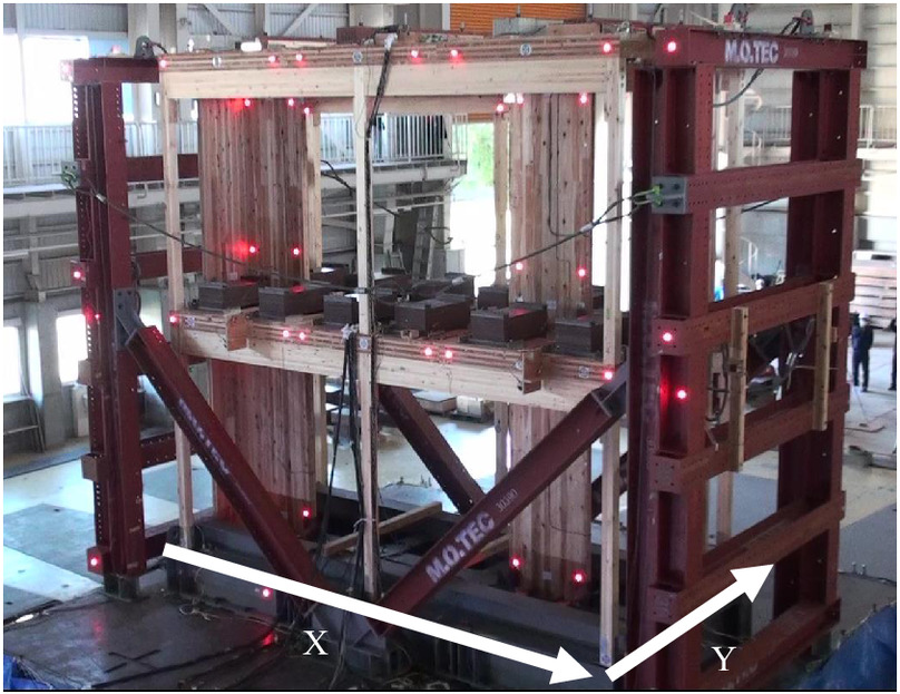
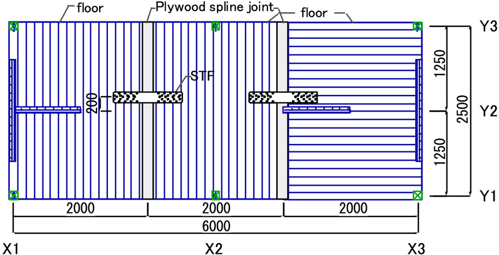
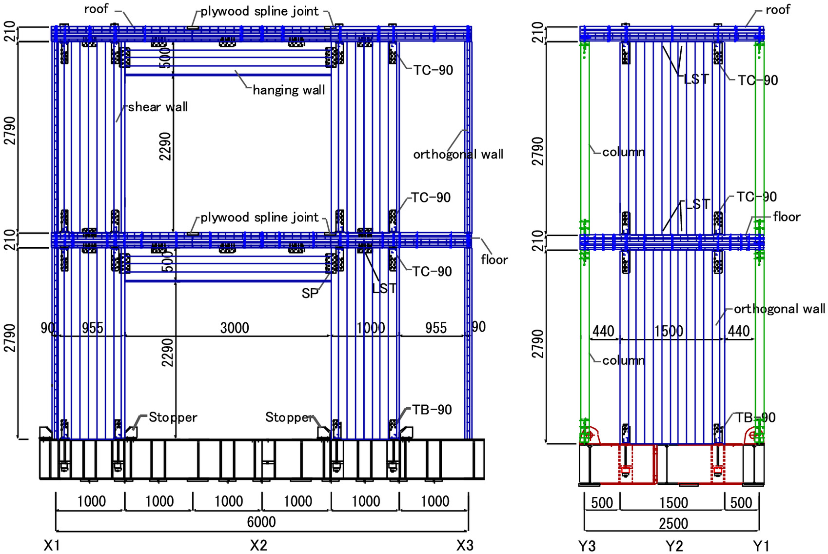
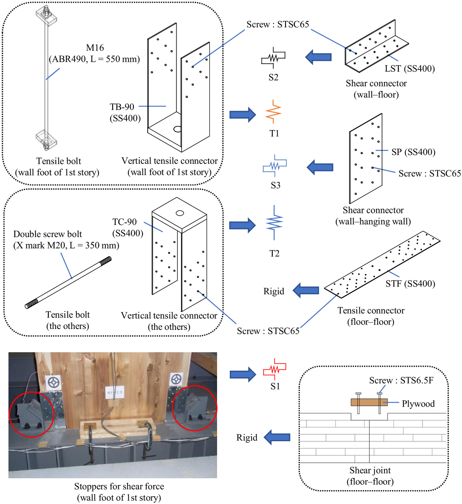
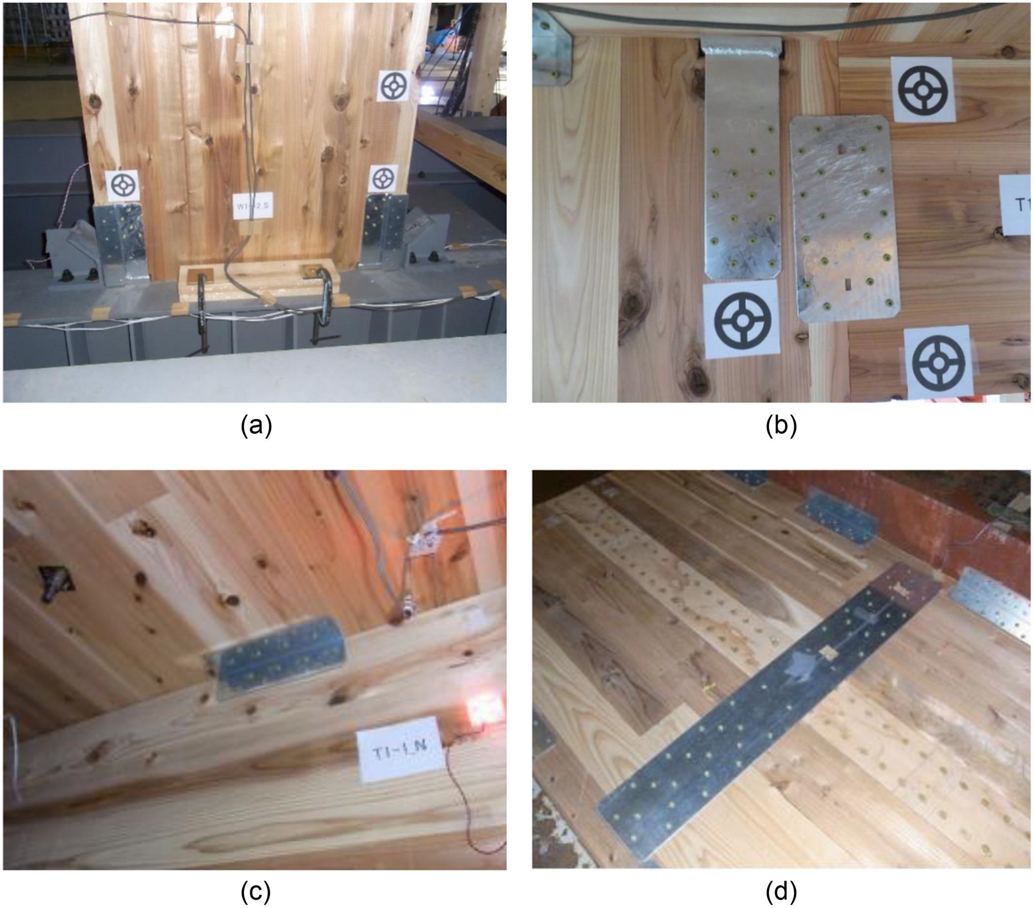
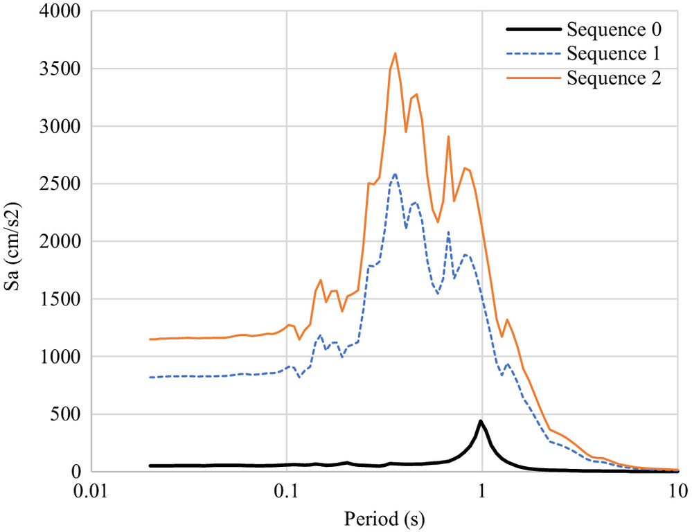
A full-scale two-story CLT building with narrow panels comprised a gravity frame, CLT wall, CLT floor, and CLT roof. The specimen and coordinate directions of the shaking table test (Fig. 2), the floor plan of the second story (Fig. 3), and its elevation in the and planes in which the CLT shear walls were located (Fig. 4) are shown. The specimen size was 6.0 m long in the -direction, 2.5 m wide in the -direction, and 6.0 m high. Two arrangements were made for the floor—one with the outermost lamina parallel to the -direction, and the other with the outermost lamina perpendicular to the -direction—to verify various conditions. As the main seismic structure, two CLT shear walls were at the center along the -direction on the first and second stories. The strength grading of glued laminated timber (glulam), which was E95-F315, is specified in the Japan Agricultural Standard (JAS). The meaning of E95 is that the laminas in all layers have an average Young’s modulus of or greater, whereas F315 indicates that the bending strength of the glulam is 31.5 MPa. The material of columns and beams was glued laminated timber made of Scotch pine (Pinus sylvestris), and had two different strength gradings, E95–F315 and E105–F300. The cross-section area was and (width × height), respectively. The horizontal diaphragm was made of seven-layer 210-mm-thick CLT panels of Japanese cedar (Cryptomeria japonica) grade Mx60 according to the JAS. The average Young’s modulus of the lamina in the outer layers was equal to or greater than , whereas it was in the inner layers. The vertical diaphragm, e.g., shear wall, hanging wall, and orthogonal wall, comprised three-layer 90-mm-thick CLT panels of Japanese cedar (Cryptomeria japonica) grade S60, meaning that the average Young’s modulus of the lamina in every lamina was equal to or greater than . Fig. 5 shows details of the connectors and the springs to which they correspond, and Fig. 6 shows images of the joints. Tensile bolts (ABR490 and M16) and U-shaped connectors (TB-90) with holes for screws were used in the wall–foundation joints. It is not common in Japan to install a stopper to resist shear force, but the purpose of this experiment was to excite the structure to a large-deformation domain. Thus, stoppers were introduced to prevent the experiment from stopping early due to the shear failure of the CLT shear wall foot of the first story [Fig. 6(a)]. The metal protectors were attached between the wall panel and stoppers to prevent the shear wall from being embedded in the stoppers due to drifting during excitation. At the wall–wall and wall–roof joints, bolts (ABR490 and M20) and U-shaped metal connectors (TC-90) with holes for screws were used as tensile connectors [Fig. 6(b)], and angle brackets (LST) with holes for screws were used as shear connectors [Fig. 6(c)]. Wall–hanging wall and floor–floor connections were made with steel plates secured with screws [Fig. 6(d)]. STS6.5F screws were used for plywood and long steel plates in the floor–floor shear joint, and STSC65 screws were used for other joints. The specimen was designed according to Route 1 provided in CLT manual (Japan Housing and Wood Technology Center 2016). Route 1 is the simple method of allowable stress design against 0.2 base shear capacity for moderate earthquake and ultimate strength design against 1.0 base shear capacity for a maximum considered earthquake. The total seismic weight of the specimen was set to 175.95 kN based on the specimen specifications of the Japanese building standard law [Notification 611 of the Ministry of Land, Infrastructure, Transport and Tourism (2016)]. The specimen was subjected to a sine wave with a frequency that was constant in Sequence 0, and to the north–south (N–S) component of JMA Kobe waves, which was recorded during the Osaka–Kobe Earthquake in 1995, at 100% and 140% intensity in Sequences 1 and 2, respectively (Table 1). The acceleration response spectrum of the three seismic waves is presented in Fig. 7. The exciting direction was the -direction of the specimen.
| Sequence | Input seismic waves |
|---|---|
| 0 | Sine wave |
| 1 | JMA Kobe 100% |
| 2 | JMA Kobe 140% |
Fourier transformation was performed on the acceleration response time history on the shaking table and on the roof of the specimen in Sequence 0, Sequence 1, and Sequence 2; then the Fourier spectrum was calculated. The Fourier spectrum of the roof was divided by that of the shaking table to obtain a spectral ratio (transfer function), and the lowest frequency among the peaks of the spectral ratio was defined as the natural frequency. In addition, the base shear capacity was derived by dividing the maximum shear force by the total seismic weight, in which the maximum shear force was determined from the acceleration observed during excitation. Table 2 shows the natural frequency and base shear capacity. The specimen’s maximum overall drift and interstory drift in Sequences 1 and 2 are listed in Table 3. During Sequence 1, the maximum roof displacement was 200 mm, corresponding to 3.33% overall drift. A split was seen at the edge of the CLT shear wall due to pulling by the hanging wall, but there was no significant damage other than the split [Fig. 8(a)]. During Sequence 2, the maximum roof displacement was 397 mm, corresponding to 6.62% overall drift, and the interstory drift of the first story was 8.77%. In addition, wall head embedment into the floor panel was observed [Fig. 8(b)]. No repair work was performed after Sequence 1. Some damage and deterioration in the specimen from Sequence 1 was considered in the analysis because the numerical models were subjected to Sequences 1 and 2 sequentially.
| Sequence | Natural frequency (Hz) | Max shear force (kN) | Total seismic weight (kN) | Base shear capacity (max shear force/total seismic weight) |
|---|---|---|---|---|
| 0 | 3.198 | — | 175.95 | — |
| 1 | 1.379 | 244.8 | 1.391 | |
| 2 | 0.9155 | 281.0 | 1.597 |
| Sequence | Max overall drift | Max interstory drift of first story | ||
|---|---|---|---|---|
| (mm) | (%) | (mm) | (%) | |
| 1 | 200 | 3.33 | 115 | 3.83 |
| 2 | 397 | 6.62 | 263 | 8.77 |

Modeling Description
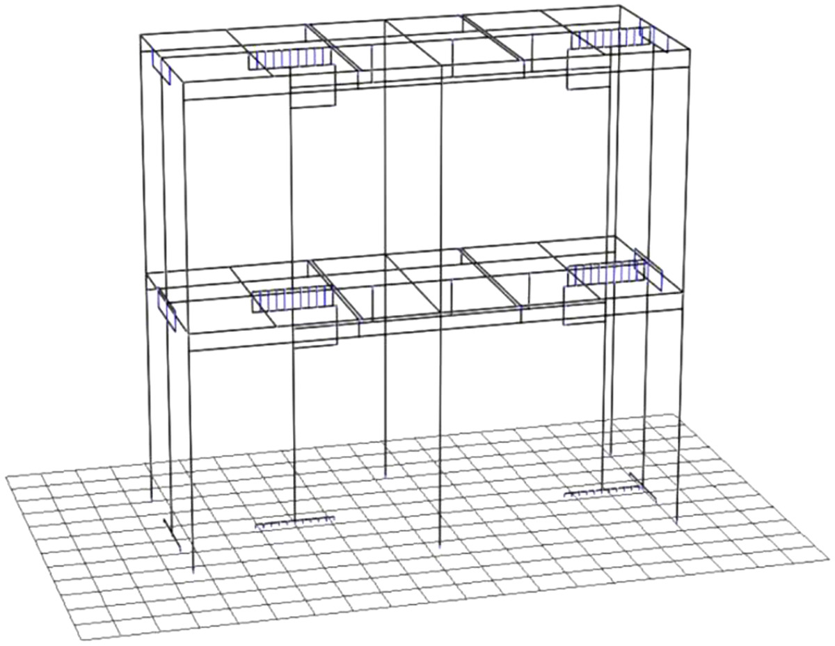
In this study, the structural analysis software wallstat was used for pushover and time-history analysis. The analysis model shown in Fig. 9 was built based on the specimen’s joint specifications. The number of nodes was 382, and the number of springs was 668. This model was fixed in the -direction of translation because twisting of the specimen was not observed in the shaking table test. Fig. 10 shows the spring arrangement in the plane. The analysis model included tensile, shear, and compression springs. Two tensile springs were used for the two types of tensile joints, wall–foundation (T1) and wall–wall or wall–roof (T2). Three types of shear springs were inserted corresponding to the stoppers in wall–foundation joints (S1) and to the shear joints with steel-plated screws in wall–floor or wall–roof joints (S2) and wall–hanging wall joints (S3). Three differently defined compression springs were inserted to express the embedment ability of CLT under loads applied to wall–foundation joints (C1), wall–floor and wall–roof joints (C2), and wall–hanging wall and orthogonal wall–floor joints (C3). Other planes, such as and , were modeled similarly.
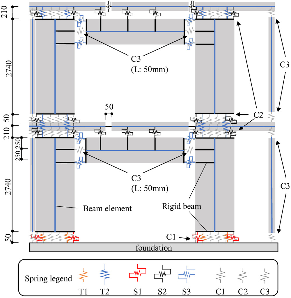
The CLT shear wall modeling method is depicted in Fig. 11, in which the CLT shear wall is modeled as a beam element with rigid beams at its top and bottom ends with lengths corresponding to the wall width. The joints at the wall head and foot were modeled with tensile springs, shear springs, and 11 compression springs. The 11 compression springs at equal intervals are called a multiple-spring; this modeling method has been used in some numerical analyses of specimens with CLT to reproduce the rocking behavior of a CLT shear wall (Sato et al. 2017; Azumi et al. 2019). The orthogonal walls, hanging walls, and floor panels were all modeled with beam elements and rigid beams, similar to the CLT shear walls. The beam elements were given only one Young’s modulus, which was applicable for both bending and compression. The Young’s modulus was set to for CLT shear walls and hanging walls, because the major direction layer was according to the CLT manual. The Young’s modulus was set to for the floor panels along the major direction, and to along the minor direction. When establishing the floor panel parameters, the cooperation width was considered. The gravity frame was modeled as a beam element with elastoplastic rotational springs at the element ends. The columns and beams’ Young’s moduli were set to 9.5 and , respectively, and the bending strength was set to 31.5 and 30.0 MPa, respectively. This Young’s modulus was applied for both bending and compression.

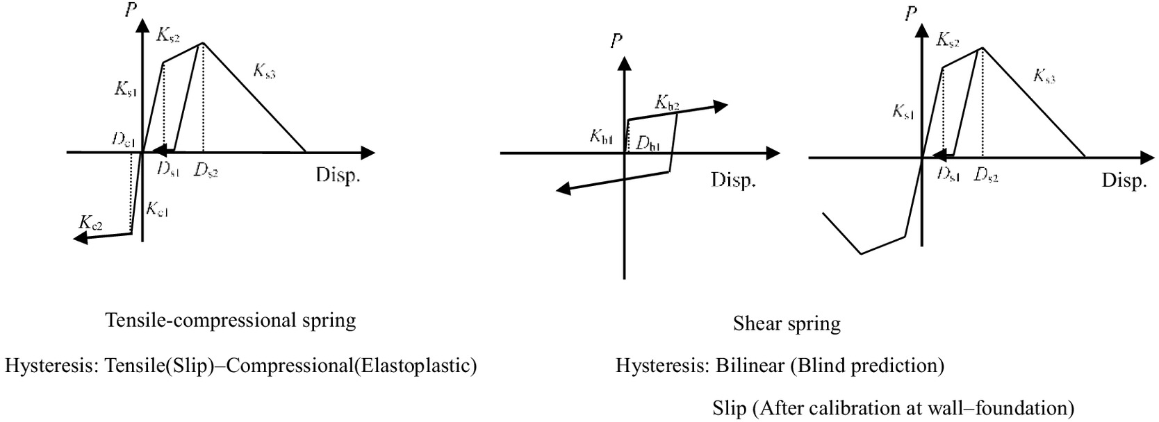
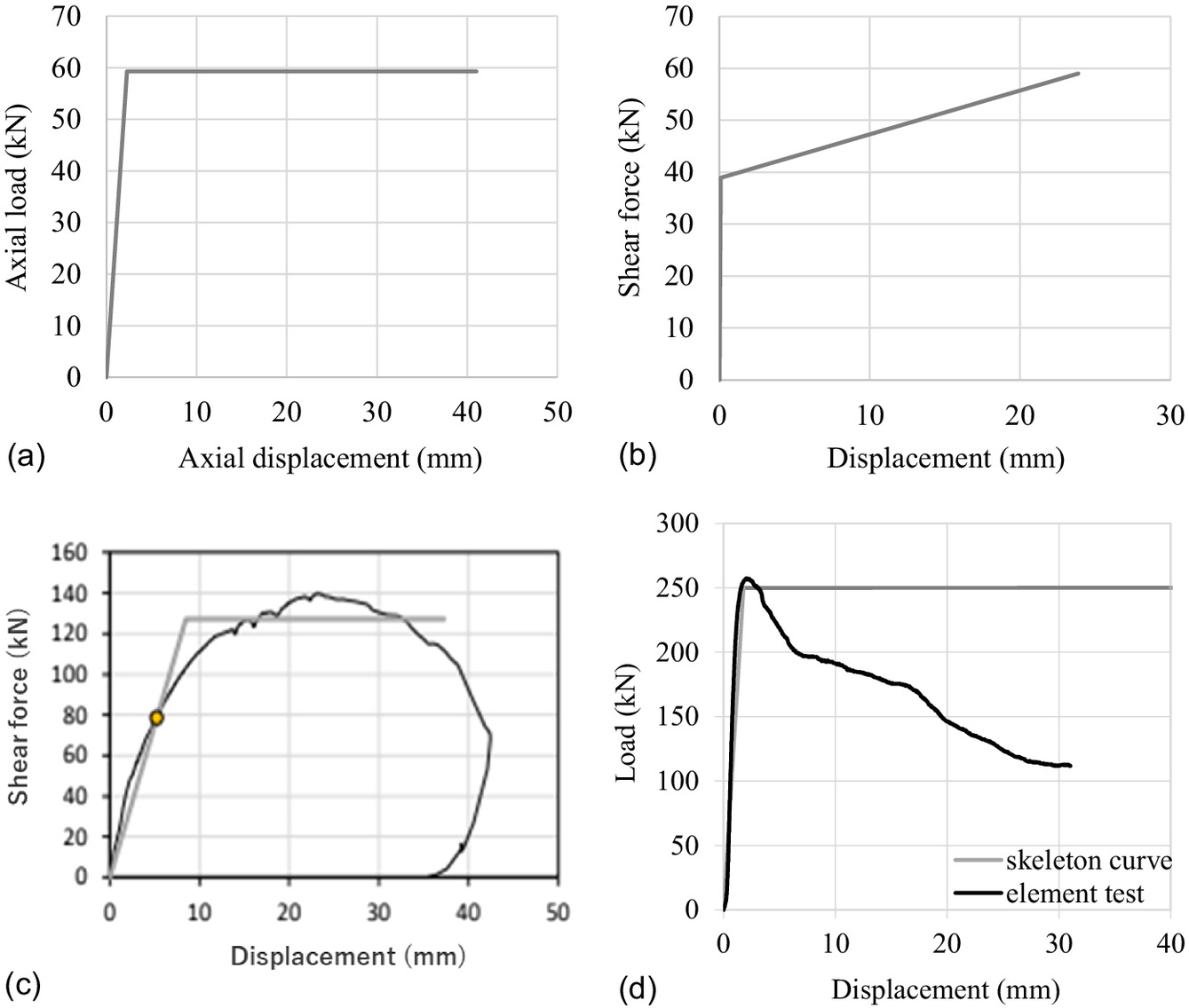
Nonlinear tensile shear springs were used to simulate each joint, and nonlinear compression springs were used to model the CLT’s embedment properties. Fig. 12 shows hysteretic rules of tensile–compressional and shear springs. The tensile–compressional spring was modeled as a slip type in tension and as elastoplastic in compression. Shear springs were set to bilinear for blind prediction, and subsequent wall–foundation shear springs were reset to the slip type considering the load–displacement relationship of the experimental results. The ultimate capacity of the tensile springs at the wall–foundation joint (T1) were determined to be 59.3 and 93 kN, and the Young’s modulus and effective area of the tensile bolts (ABR490 and M16) were and , respectively, according to JIS B 1220 (JISC 2010). In addition, the length between the nuts was 400 mm; therefore, the first stiffness and the ultimate displacement for the T1 spring were set to and 41 mm, respectively, based on the CLT manual. Similarly, for the wall–wall joint (T2), the Young’s modulus and effective area of tensile bolts (ABR490 and M20) were and , respectively, according to JIS B 1220, and the length between the nuts was 200 mm. Therefore, the first stiffness and the ultimate displacement for the T2 spring were set to and 20 mm, respectively, according to the CLT manual. For the shear springs at the wall–floor joints (S2), the yielding and ultimate capacity of the two angle brackets were determined to 54 and 90 kN, respectively, based on the CLT manual. In addition, considering friction, the first stiffness was assumed to be rigid, and the value obtained by multiplying the allowable (79.6 kN) and ultimate capacities (93.0 kN) of the tensile joint from JIS B 1220 by a friction coefficient of 0.3 were added to 54 and 90 kN, giving 77.9 and 118 kN. Because the four shear springs were distributed at the wall–floor joints (Fig. 11), the calculated yielding and ultimate capacities were divided by 2. Finally, yielding and ultimate capacities for the shear spring were set to 38.9 and 59.0 kN.
The ultimate displacement was set to 23.86 mm based on the CLT manual. Skeleton curves of the wall–hanging wall shear spring (S3) and wall–foundation compression spring (C1) were determined from the element test results [Figs. 13(c and d)]. The critical tensile–compressional and shear spring properties in this analysis model are presented in Tables 4 and 5. All analytical results were generated using a time-integration step of . The numerical analysis used the measured acceleration at the center of the shaking table as ground motions. The model weights were equal to the seismic weights of the full-scale specimen, including members and loaded weights, and the weights of the first and second stories were set to 100.54 and 75.41 kN, respectively.
| Spring | First stiffness, () | Seccond stiffness, () | Third stiffness, () | First yield point, (mm) | Second yield point, (mm) | Ultimate displacement, (mm) | First compression stiffness, () | Second compression stiffness, () | First yield point, (mm) |
|---|---|---|---|---|---|---|---|---|---|
| Wall–foundation (T1) | 26 | 0.001 | 2.3 | 40 | 41 | 0.001 | — | — | |
| Wall–wall (T2) | 30 | 0.001 | 3.1 | 10 | 20 | 0.001 | — | — | |
| Wall–foundation (C1) | 0.001 | 0.0001 | 13.5 | 21.6 | 1000 | 140.4 | 0.001 | 1.78 |
| Spring | First stiffness, () | Second stiffness, () | First yield point, (mm) | Ultimate displacement, (mm) |
|---|---|---|---|---|
| Wall–foundation (S1) | Rigid | |||
| Wall–floor (S2) | 486.75 | 0.8445 | 0.08 | 23.86 |
| Wall–hanging wall (S3) | 15 | 0.001 | 8.5 | 37 |
Analysis Based on the Element Test Results and Reference Value (Blind Prediction)
Pushover analysis was performed on the analysis model based on the element test results and reference value, i.e, blind prediction. Fig. 14 depicts the blind prediction and hysteresis of the experiment on the story shear force–interstory drift for the first and second stories. The hysteresis of the experimental results was drawn using the acceleration and displacement measured in the shaking table tests. The first stiffness agreed with the experiments for both the first and second stories, but the maximum capacity of the second story and the ductility of the first and second stories were insufficient, indicating that the analysis could not reproduce the full-scale shaking table test results as described by Yasumura et al. (2016) when the parameters of the spring were determined by element test results. Thus, reproductive analysis was performed to better match the experimental results.
Reproductive Analysis
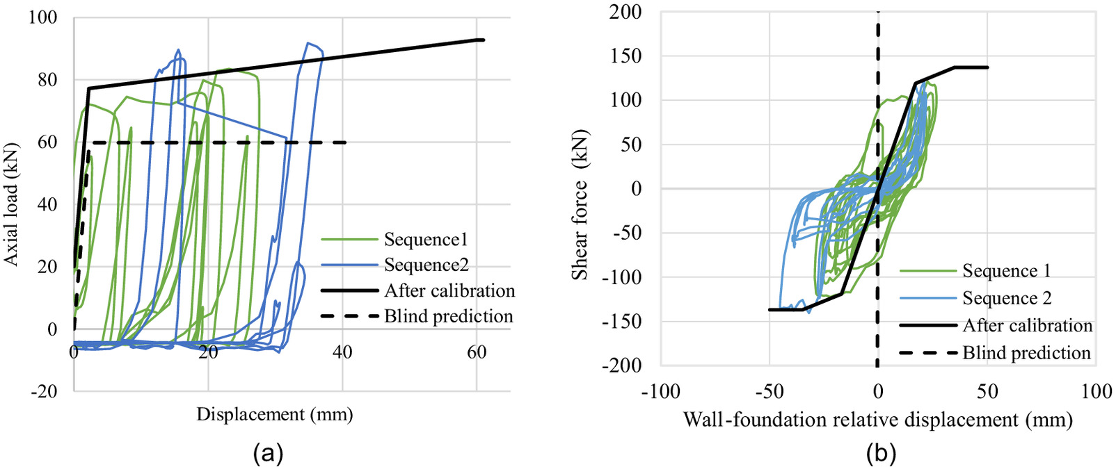
As previously stated, pushover analysis based on elemental tests and references could not reproduce the behavior of full-scale shaking table test at large deformation. The shaking table test results were used to calibrate the spring parameters for the wall–foundation tensile and shear joints (Fig. 15). For the tensile spring, the axial force–displacement relationship of the tensile bolts at the wall–foundation was traced, and the skeleton curve was defined by the slip-type hysteresis characteristics. In addition, a pre-tension load of 20 kN was added according to the experimental condition. Half of the shear force for the first story against wall–foundation relative displacement was traced for the shear spring skeleton curve. Half of that was used because there were two CLT shear walls on the first story. The skeleton curve was defined by the slip-type hysteresis characteristics. Table 6 presents the two spring properties after calibration. Comparing the skeleton curve in blind prediction and after calibration showed that the tensile spring parameters after calibration matched well with those in blind prediction. For the shear spring, the difference in the first stiffness was large, indicating that the shear resistance ability of the stoppers was not rigid due to the embedment of the CLT shear wall even if the metal protectors were installed.
| Spring | First stiffness, () | Secnd stiffness, () | Third stiffness, () | First yield point, (mm) | Second yield point, (mm) | Ultimate displacement, (mm) | Compression stiffness, () |
|---|---|---|---|---|---|---|---|
| Wall–foundation (T1) | 26 | 0.2685 | 2.2 | 60 | 61 | 0.001 | |
| Wall–foundation (S1) | 7 | 1 | 17 | 35 | 50 | — |
Furthermore, to enhance reproducibility, the analytical method of Namba et al. (2021), data assimilation, was performed for the reproductive analysis. The 24 critical parameters of springs and elements in Table 7 were the target of data assimilation, and were multiplied by the correction factors to create various skeleton curves, and the parameter conbinations when fit to the experimental results were explored. The correction factors had the range to account for variations in materials and resistance factors which were not considered in the analytical model. Assuming that the variation due to these uncertainties was expressed as the correction factors’ coefficient of variation and that the mean value of the correction factors was 1, the standard deviation was derived using Eq. (1). Assuming that the correction factor was normally distributed, standardization was performed using the random variable according to Eq. (2). In this case, accounted for 99.38% of the total, which covered almost all patterns. Therefore, the correction factors were varied in the range 0.5–2.0 in intervals of 0.15 for the Young’s modulus, first stiffness, and first yield point. For the second stiffness, the correction factors were varied in the range 0.0001–0.8 in intervals of 0.08, considering that the most possible values of the stiffness after yielding were covered
(1)
(2)
| Spring position | Joint type | Spring type | Multiplied parameters |
|---|---|---|---|
| CLT shear wall | — | Beam element | Bending Young’s modulus |
| Hanging wall | — | Beam element | Bending Young’s modulus |
| Floor panel, beam | — | Beam element | Bending Young’s modulus |
| Wall–wall | Tensile | Tensile–compressional | , , |
| Wall–hanging wall | Tensile | Tensile–compressional | , , |
| Column foot | Tensile | Tensile–compressional | , , |
| Wall–wall | Shear | Shear | , , |
| Wall–hanging wall | Shear | Shear | , , |
| Wall–foundation | Compression | Tensile–compressional | , , |
| Wall–hanging wall | Compression | Tensile–compressional | , , |
With this method, various skeleton curves for the springs were created. Then the experimental results and many analytical results were compared in terms of only the shear force–interstory drift of the first story through Sequences 1 and 2, not in terms of the time history of interstory drift and uplift displacement. Then the analytical results with the smallest error from the experimental results were extracted. By comparing the skeleton curves before assimilation and after assimilation, five analysis results with the five smallest errors from the experimental results were extracted. Thus, assimilation was performed to match both Sequences 1 and 2. Therefore, the damage from Sequence 1 also was considered in the analytical results after data assimilation. In addition, because all springs and elements were free in all directions except the -direction of translation, if multiple factors are included in the springs and elements, data assimilation of the parameters will result in an accurate analysis model.
The interstory drift time history for the first and second stories in Sequences 1 and 2 from data assimilation is illustrated in Fig. 16, together with the blind prediction and experimental results. The blind prediction did not agree with the experiment results except for the initial drift response to the excitation. After assimilation, both the interstory drift and phase agreed well with the experimental results through Sequence 1. In Sequence 2, there was a slight error in interstory drift with the experiment results after the maximum drift, but the trends of the interstory drift and phase agreed well, implying a good reproduction result.
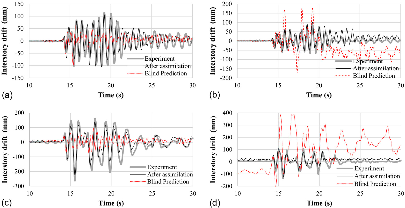
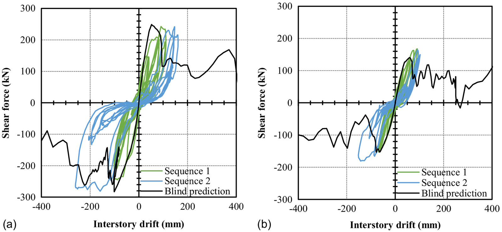
Fig. 17 illustrates the shear force–interstory drift relationships for the first story in Sequences 1 and 2 in the experiment, in blind prediction, and after assimilation. For the blind prediction, the maximum load was nearly reproduced in Sequence 1, but not in Sequence 2. Nevertheless, the interstory drift and stiffness were not consistent with the experiment results. However, the analytical results after assimilation were almost identical to the experimental result, indicating that the overall behavior of the specimen could be tracked by reproductive analysis.
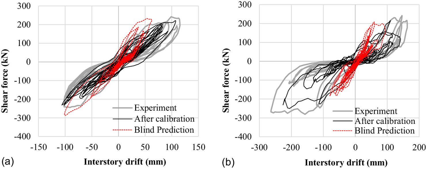
Fig. 18 shows the uplift displacement time history at the CLT shear wall foot of the first story in Sequence 2 in the experiment and the analysis results after assimilation. The analytical result after assimilation agreed with the experimental results in drift and phase, demonstrating that the detailed behavior of the two-story CLT building was reproduced.
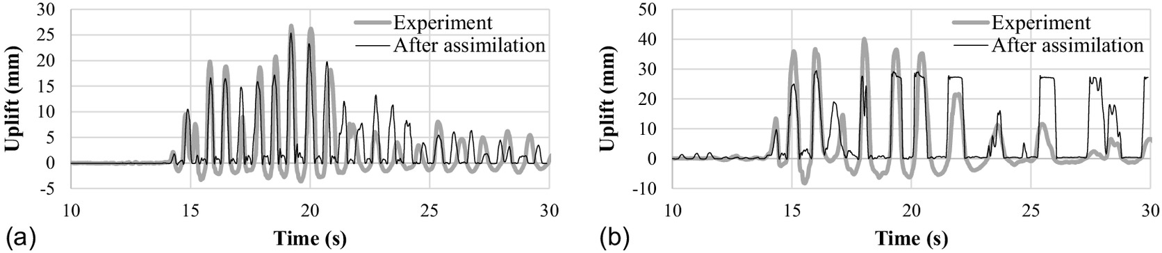
Fig. 19 shows the skeleton curves for the four springs before and after assimilation. The solid lines in Figs. 19(a–d) are skeleton curves in the analysis results with the five smallest errors from the experimental results. The five analytical results (labeled 1–5 in order from the smallest to the fifth smallest) are shown to indicate the trend of how the skeleton curves changed.
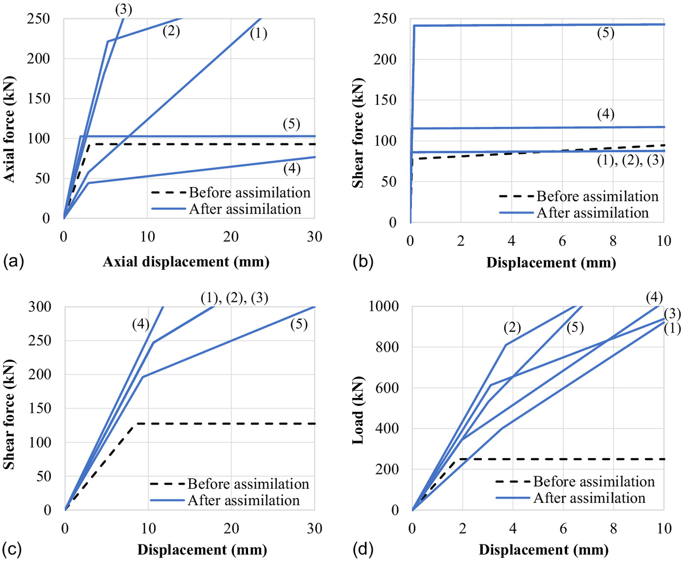
For the wall–wall tensile springs [Fig. 19(a)], a clear trend of the first stiffness and yielding capacity was not seen. For the wall–floor shear spring [Fig. 19(b)] considering friction when determining the parameters, the skeleton curves tended to be the same before and after assimilation. For the wall–hanging wall shear spring [Fig. 19(c)] without considering friction, both stiffness and yield capacity tended to increase after assimilation. This implies that the friction between the shear connectors under suppressed force contributed to an increase in both stiffness and yielding capacity. However, it is recommended to reconsider the friction coefficient, which was 0.3 in this paper. In addition, the difference in the loading speed between the dynamic loading during the full-scale shaking table test and the static loading in the element tests can be another reason for increase of the stiffness and yielding capacity. In additioin, for Analytical result 5, the yielding capacity of the wall–floor shear spring was the highest, although the first stiffness and yielding capacity of the wall–hanging wall shear spring were the smallest, implying that the wall–floor and wall–hanging wall shear springs had an inverse relationship.
An increasing trend of the first stiffness and yielding capacity also was seen in the case of the compression springs [Fig. 19(d)]. Similar to the shear springs, the dynamic effects of loading can be a contributing factor to the increase in stiffness and yielding capacity. Another possible factor is that the dead weights were fixed to the floor with screws in the experiment, which increased the floor rigidity significantly and suppressed the vertical deformation caused by the rocking of the CLT shear walls. These inverse interactions and factors for increase of stiffness and capacity, such as friction, dynamic effects, and increase of floor rigidity, will be verified by comparing the detailed behavior and performing static loading tests in the future.
Conclusion
This study proposes a model that can replicate the seismic behavior of CLT buildings up to a large-deformation region using wallstat, which was modified to consider the restoring force and effects due to the rocking behavior of CLT panels. The shaking table test of a two-story full-scale CLT building validated the analytical method. The results were as follows:
•
A split was observed at a wall–hanging wall joint. Despite the 8.77% interstory drift of the first story in Sequence 2, further damage, such as wall head embedment into the floor panel, was negligible.
•
In pushover analysis, blind prediction agreed well with the experimental result in terms of the first stiffness but not with the maximum capacity of the second story and the ductility of the first and second stories.
•
The shaking table test results of the two-story full-scale CLT building were analyzed using wallstat, which was modified to include multiple-spring and shear spring models, to account for restoring force and effects due to the rocking behavior of the CLT panels. Using wallstat, we replicated the seismic behavior of the two-story full-scale CLT building up to a large-deformation domain. Blind prediction could not reproduce the experimental results in the time-history interstory drift and hysteresis curves of the shear force–interstory drift of the first story. However, the analytical results after assimilation were consistent with the experimental results in interstory drift and phase in both the first and second stories, demonstrating that the overall behavior of the CLT building specimen was reproduced with this analytical method even in the large-deformation domain. The discrepancy between the analysis and experiment after the maximum drift will be the subject of future research,
•
The uplift displacement and phase trends of the CLT shear wall of the first story were analyzed for the uplift displacement time history. The outcomes suggest that our analysis model can replicate even the detailed behavior of a full-scale specimen at large deformation as well as the overall behavior.
•
The skeleton curves of shear and compression springs after data assimilation tended to increase in both stiffness and yielding load compared with those before assimilation. The suppression of deformation due to friction resistance, the difference in the loading speed between the element tests and the shaking table test, and the increment in floor rigidity due to fixed dead weights were considered to be the cause of these increases.
The analysis results after assimilation agreed well with the experimental results, indicating the validity of this study’s analytical method. However, it is not possible to predict the responses of CLT buildings without experimental results solely using this study. In this study, as a result of varying the chatacteristic values for joints and members over the statistically determined range, analytical results that agreed with the experimental results were obtained, and the trend of the analytical results was shown. Friction, dynamic effects, and an increase in floor rigidity due to fixed dead weights were thought to be the causes of the increasing trend of stiffness and yielding capacity of shear and compression spring. In addition, because an inverse relationship between the properties of the shear springs was confirmed, interaction among the tensile, shear, compression springs, and beam elements also can exist. These interactions in analysis models of this study have to be verified in the future through behavior comparisons of detailed part and static loading tests, and it is believed that the verification will lead to the abailty to predict the seismic behavior of CLT buildings at large deformation without experimental results.
Data Availability Statement
Some or all data, models, or code that support the findings of this study are available from the corresponding author upon reasonable request.
Acknowledgments
This research was conducted as part of a Forestry Agency–subsidized project to study the relaxation of earthquake resistance standards by simplifying joints, reducing the number of walls, and so forth based on an understanding of the seismic boundary performance of CLT panel construction method buildings. to the authors express their gratitude to all the parties involved. The Japan Aerospace Exploration Agency supercomputer system JSS3 was used for the reproductive analysis.
References
Azumi, Y., T. Miyake, K. Matsumoto, I. Sakurai, and N. Kawai. 2019. “A study on expansion and improvement of the structural design method for CLT panel construction, Part 2 Simplification of numerical analysis model by Multiple Spring element.” [In Japanese.] In Proc., Summaries of Technical Papers of Annual Meeting, 461–462. Tokyo: Architectural Institute of Japan.
Blomgren, H. E., S. Pei, Z. Jin, J. Powers, J. Dolam, J. W. van de Lindt, A. R. Barbosa, and D. Huang. 2019. “Full-scale shake table testing of cross-laminated timber rocking shear walls with replaceable components.” J. Struct. Eng. 145 (10): 04019115. https://doi.org/10.1061/(ASCE)ST.1943-541X.0002388.
Ceccotti, A. 2008. “Few technologies for construction of medium-rise buildings in seismic regions.” Struct. Eng. Int. 18 (2): 156165. https://doi.org/10.2749/101686608784218680.
Ceccotti, A., and M. Follesa. 2006. “Seismic behavior of multi-story XLAM buildings.” In Proc., Int. Workshop on Earthquake Engineering on Timber Structures. Coimbra, Portugal: Univ. of Coimbra.
Ceccotti, A., C. Sandhaas, M. Okabe, M. Yasumura, C. Minowa, and N. Kawai. 2013. “SOFIE 3D shaking table test on a seven-storey full-scale cross-laminated timber building.” Earthquake Eng. Struct. Dyn. 42 (13): 2003–2021. https://doi.org/10.1002/eqe.2309.
Cundall, P. A. 1971. “A computer model for simulating progressive large-scale movements in blocky rock system.” In Proc., Symp. ISRM, 129–136. Lisbon, Portugal: International Society for Rock Mechanics and Rock Engineering.
Dujic, B., K. Strus, R. Zarnic, and A. Ceccotti. 2010. “Prediction of dynamic response of a 7- storey massive XLAM building tested on a shaking table.” In Proc., WCTE 2010, World Conf. on Timber Engineering. Torento, Italy: Riva del Garda.
Hidaka, T., T. Nakagawa, and M. Inayama. 2013. “Damage investigation and collapsing process analysis of Myokenji Hondo damaged from the Great East Japan EARTHQUAKE: Part 1 Damage investigation and measurement survey.” [In Japanese.] J. Struct. Eng. 59: 567–572.
Japan Housing and Wood Technology Center. 2016. Design and construction manual for CLT buildings. Koutou ward, Tokyo: Japan Housing and Wood Technology Center.
JISC (Japanese Industrial Standards Committee). 2010. Set of anchor bolt with rolled threads for structures. JIS B 1220. Tokyo: JISC.
Meguro, K., and M. Hakuno. 1991. “Simulation of structural collapse due to earthquakes using extended distinct element method.” [In Japanese.] In Proc., Summaries of Technical Papers of Annual Meeting, 763–764. Tokyo: Architectural Press Institute of Japan.
Nakagawa, T., T. Hidaka, and M. Inayama. 2013. “Damage investigation and collapsing process analysis of Myokenji Hondo damaged from the Great East Japan EARTHQUAKE: Part 2 Collapsing process analysis using 3D space frame model.” [In Japanese.] J. Struct. Eng. 59: 573–578.
Nakagawa, T., and M. Ohta. 2003a. “Collapsing process simulations of timber structures under dynamic loading I: Simulations of two-story frame models.” J. Wood Sci. 49 (5): 392–397. https://doi.org/10.1007/s10086-002-0500-z.
Nakagawa, T., and M. Ohta. 2003b. “Collapsing process simulations of timber structures under dynamic loading II: Simplification and qualification of the calculating method.” J. Wood Sci. 49 (6): 499–504. https://doi.org/10.1007/s10086-002-0507-5.
Namba, T., T. Nakagawa, Y. Kado, A. Takino, and H. Isoda. 2021. “Study of data assimilation method for the collapsing simulation of wooden houses using the quality engineering: Part5 Shaking table tests on wooden structure consisting of moment-resisting frames.” In Proc., Summaries of Technical Papers of Annual Meeting, 301–302. [In Japanese.] Tokyo: Architectural Institute of Japan.
Pei, S., M. Popovski, and J. W. van de Lindt. 2013. “Analytical study on seismic force modification factors for cross-laminated timber buildings.” Can J. Civ. Eng. 40 (9): 887–896. https://doi.org/10.1139/cjce-2013-0021.
Popovski, M., and I. Garvic. 2016. “Performance of two-storey CLT house subjected to lateral loads.” J. Struct. Eng. 142 (4): 2016. https://doi.org/10.1061/(ASCE)ST.1943-541X.0001315.
Rinaldin, G., and M. Fragiacomo. 2016. “Non-linear simulation of shaking-table tests on 3- and 7-storey X-LAM timber buildings.” Eng. Struct. 113 (15): 133–148. https://doi.org/10.1016/j.engstruct.2016.01.055.
Sato, M., H. Isoda, Y. Araki, T. Nakagawa, N. Kawai, and T. Miyake. 2019. “A seismic behavior and numerical model of narrow paneled cross-laminated timber building.” Eng. Struct. 179 (15): 9–22. https://doi.org/10.1016/j.engstruct.2018.09.054.
Sato, M., H. Isoda, Y. Araki, T. Nakagawa, and T. Miyake. 2017. “Proposal of analysis model of CLT structure for small width panel and accuracy verification intended.” [In Japanese.] J. Struct. Constr. Eng. 82 (741): 1719–1726. https://doi.org/10.3130/aijs.82.1719.
Sumida, K., T. Nakagawa, and H. Isoda. 2020. “Seismic testing and analysis of rocking motions of Japanese after and-beam construction.” J. Struct. Eng. 147 (2): 04020323. https://doi.org/10.1061/(ASCE)ST.1943-541X.0002901.
Yasumura, M., K. Kobayashi, M. Okabe, T. Miyake, and K. Matsumoto. 2016. “Full-scale tests and numerical analysis of low-rise CLT structures under lateral loading.” J. Struct. Eng. 142 (4): E4015007. https://doi.org/10.1061/(ASCE)ST.1943-541X.0001348.
Zhang, X., H. Isoda, K. Sumida, Y. Araki, S. Nakashima, T. Nakagawa, and N. Akaiyama. 2021. “Seismic performance of three-story cross-laminated timber structures in Japan.” J. Struct. Eng. 147 (2): 04020319. https://doi.org/10.1061/(ASCE)ST.1943-541X.0002897.
Information & Authors
Information
Published In

Journal of Structural Engineering
Volume 149 • Issue 6 • June 2023
Copyright
This work is made available under the terms of the Creative Commons Attribution 4.0 International license, https://creativecommons.org/licenses/by/4.0/.
History
Received: May 31, 2022
Accepted: Jan 26, 2023
Published online: Apr 6, 2023
Published in print: Jun 1, 2023
Discussion open until: Sep 6, 2023
ASCE Technical Topics:
- Building materials
- Continuum mechanics
- Deformation (mechanics)
- Earthquake engineering
- Engineering fundamentals
- Engineering materials (by type)
- Engineering mechanics
- Geomechanics
- Geotechnical engineering
- Laboratory tests
- Laminating
- Materials engineering
- Materials processing
- Seismic effects
- Seismic tests
- Shake table tests
- Soil dynamics
- Soil mechanics
- Solid mechanics
- Structural engineering
- Structural mechanics
- Structures (by type)
- Tests (by type)
- Uplifting behavior
- Wood and wood products
- Wood structures
Authors
Metrics & Citations
Metrics
Citations
Download citation
If you have the appropriate software installed, you can download article citation data to the citation manager of your choice. Simply select your manager software from the list below and click Download.