Improved Method of Determination of Basic Wind Speed with Terrain Effects Using Graph Neural Network
Publication: Journal of Structural Engineering
Volume 149, Issue 1
Abstract
In determining wind loads when designing buildings—especially high-rise buildings—wind speed is a critical factor. With increased progression of city high-rise construction, accurate prediction has become ever more important. Many factors, such as local climates, roughness of surrounding conditions, and terrain, may affect wind speed. But among all factors considered, terrain has a very large influence. Difficulties in reflecting the influence of terrain on wind speed include (1) collecting topographic data information; (2) quantitatively evaluating terrain features; and (3) expressing specific area relationships with surrounding observation stations. This paper poses means to solve these limitations by (1) using satellite imagery to gather topographic information; (2) evaluating terrain quantitatively with convolutional neural network (CNN)–based encoders; and (3) employing a graph neural network (GNN) to estimate the wind speed relationship of an arbitrary place to that of observation stations. Herein, a machine learning model utilizing the aforementioned means was proposed. To support this model, an experiment was conducted using observed wind speed data in Korea. Throughout the experiment, previous studies were used to compare results with ratification of the posed model. Given the submitted findings, further research and investigation to establish correlation with other experimental case results are proposed.
Introduction
Due to urbanization, an increase in the number of high-rise buildings constructed is projected. Given their vulnerability to wind loads, precise determination becomes increasingly important. As is, wind load is determined from the basic wind speed of a site and varies with regional climate. Because wind velocity pressure is proportional to the square of wind speed, small discrepancies or errors in determining basic wind speed may result in large differences in wind load. When considering gust effects and vortex-induced vibrations, these differences can be even greater (Bahmani et al. 2014; Bernardini et al. 2015; Kwon et al. 2015; Lou et al. 2015; Alinejad and Kang 2020; Ouyang and Spence 2020; Cui and Caracoglia 2020; Jeong et al. 2021). Because vortex shedding is affected by building shape, characteristic length, and wind speed, with a fixed shape and length of target structure, the wind speed is a main governing factor.
For tall and slender buildings with rectangular shapes, more eminent vortex shedding can occur due to two-dimensional air flow at the midsection. Tall buildings exceeding 30 stories are governed by across-wind loads induced by vortex shedding (Kang et al. 2019). Including gust effects, vortex-induced wind load, and resonance of the structure, the maximum displacement by along-wind load is proportional to 2.1 power of mean wind speed (or basic wind speed), and that by across-wind (vortex-induced vibration) is proportional to 3.1 power of mean wind speed (Tamura 2020). Underestimation or overestimation of wind loads can be directly related to safety or cost issues even for low-rise buildings and wind turbines in mountains. Thus, accurate determination of basic wind speed is significant in wind engineering.
Basic wind speeds in the form of maps or tables are provided in national design codes and standards. These speeds are derived from wind speed data collected at observation stations. The raw data of observed wind speeds involve not only climate characteristics, but also effects of surrounding site conditions (called surface roughness) and topography at the station. The effects of roughness and topography on wind speed profiles and mean wind speeds are explained in Engineering Sciences Data Unit (ESDU) publications ESDU 84011 (ESDU 2012) and ESDU 91043 (ESDU 2000). ESDU 84011 (ESDU 2012) presents wind speed profile modification depending on roughness and varying roughness in upwind site. ESDU 91043 (ESDU 2000) provides simplified and detailed methods to consider the effect of topography. For use in design codes, standardization of terrain effects and modification of the wind speed data is carried out. After modification, an extreme value analysis to estimate the expected maximum wind speed for the target return period is conducted. Accurate estimations require sufficient data recorded over decades. Determination of basic wind speed on a national scale requires significant judgment and effort from engineers. Thus, the results of the process may differ depending on the engineers.
One of the most challenging issues for determination of basic wind speed is homogenization of site conditions. In design codes, basic wind speed is defined as mean wind speed (averaging time varies with design codes) at 10 m above the ground in open terrain. Thus, wind speed data from observation stations should be modified for homogenized site conditions. There are code-specified regulations for modification of wind speed considering neighboring surface roughness and topography. However, it is difficult to apply the regulations to real-world circumstances due to its complexity. At this stage, judgment for classification of surface roughness or determination of topography factor can vary depending on engineers.
Additionally, selection of data is important. The traditional method uses wind speed data from the nearest observatory station regardless of terrain features. However, modification equations to account for terrain features may not be accurate in three-dimensional complicated terrains. Referring to wind speed data from stations with similar terrain features can result in better estimation (Lee et al. 2022).
To address the aforementioned issues, this study attempts to improve the method of determination of basic wind speed using machine learning. Terrain features from satellite images are evaluated by convolutional neural network (CNN)–based encoders, and particularly, graph neural network (GNN) is used to express the relationship between stations.
Existing Research on Prediction of Wind Speed and Its Limitations
As mentioned previously, wind speed is significantly affected by surrounding site conditions, such as surface roughness and topography. Most prior studies were conducted to figure out the effect of topography, for which wind tunnel tests and computational fluid dynamics (CFD) analysis were commonly used (Bowen and Lindley 1976; Carpenter and Locke 1999; Wang et al. 2014; Wani et al. 2021). However, the research was mainly focused on two-dimensional (2D) hill or escarpment effects. For more complex conditions combined with surface roughness, Abdi and Bitsuamlak (2014) conducted CFD analysis to examine the effect of roughness change; however, CFD analysis has limitation of requiring a large amount of computational time and cost.
Research comparing national basic wind speeds has been conducted in the past. Almaawali et al. (2008) compared basic wind speeds in Oman determined by Gumbel and Gringorten methods. Lakshmanan et al. (2009) updated India’s basic wind speed map by using long-term hourly wind data. However, research conducted by Almaawali et al. (2008) and Lakshmanan et al. (2009) did not mention the standardization of terrain conditions in modification of wind speed data. On the other hand, Ballio et al. (1999) presented basic wind speeds in Italy based on the distance from the sea and altitude. Jeong et al. (2014) suggested an effective height concept to modify wind speed data for standardized terrain conditions. Although terrain conditions were considered in these studies, how complex three-dimensional (3D) terrain in the real world was quantified and classified by authors is not clearly known.
For problems difficult to quantify or solve by human intuition, artificial intelligence has begun to be used. Especially, machine learning is rapidly developed and applied to various fields. Koo et al. (2015) adopted the method of artificial neural networks to predict wind speed based on distance according to the type of topography and discussed the relationship between them. By studying each topography type, Koo et al. (2015) indirectly confirmed its importance when predicting wind speed. This study had the following limitations: (1) wind speed data were categorized roughly into three types of coast, plain, and mountain; (2) the data used were only numerical data in terms of distance between two points, observed wind speed data, etc.; and (3) only 6 years of the observed data were used.
Lee et al. (2022) proposed the method of evaluating and predicting topography similarity using satellite images and a CNN-based neural network. The model suggested by Lee et al. (2022) did not acquire a direct relationship between wind speed and topography. The topography features of satellite images were learned through a CNN, and the 100-year return period wind speed of a certain region was predicted. The model adopted a two-staged method that first extracts and learns topographic features of images using autoencoder (AE) to distinguish topography features from satellite images and estimate wind speeds at specific locations by linearly combining learned topographic information with location information of the station. In this study, the selection of observation station was significant for accuracy, and three methods to select a reference station for basic wind speed prediction were proposed as follows: (1) selecting the nearest station from the target site (select one); (2) using wind speed data from nearby of stations [ neighbor ()]; and (3) selecting of stations considering distance and terrain similarity. The method of simply utilizing the data of the nearest station showed a considerably large error, and the method of utilizing the data of the nearest of stations increased in accuracy as increased, but still showed an error of 3.26 to . In case that terrain similarity was additionally considered, the predicted basic wind speed (average ) showed higher accuracy than that of the previous two methods.
Because the aforementioned methods are two-staged methods using CNN, they require user intervention. Lee et al. (2022) also proposed an end-to-end method that treats from input to output as a single neural network without a segmented network, and to this end, multilayer perceptron (MLP) was used. The predicted wind speed through the MLP method was compared with observed data, and the accuracy was significantly higher than that of all other previous methods (average ). Therefore, it is considered that the end-to-end method using a single neural network is more efficient for predicting the basic wind speed using satellite images. However, because the MLP method only derives one value of 100-year return period basic wind speed, limitation exists in that multiyear data of specific location cannot be predicted.
This study proposes an improved end-to-end model that complements the aforementioned limit. The main characteristics of the model proposed in this study are as follows:
•
The process of extracting features from satellite images to the process of predicting wind speed is a single deep learning model (end-to-end model).
•
Graphical representation of observation stations are in the form of unstructured data using GNN.
•
Wind speed records for the last 19 years were used for estimation in lieu of a basic wind speed based on the probability model.
•
Multiyear annual maximum wind speed can be predicted.
Limitations of Existing Basic Wind Speed Determination Method
Existing Basic Wind Speed Determination Process
Current design codes and standards reference wind speed for the region to be used in all site conditions as the basic wind speed. It is standardized for specific site conditions. In design codes and standards such as ASCE 7-22 (ASCE 2022), Architectural Institute of Japan (AIJ) AIJ-RLB (AIJ 2015), Eurocode 1 (CEN 2003), Korean Design Standard [KDS 41:2019 (MOLIT 2019)], and ISO 4354 (ISO 2009), basic wind speed is defined as wind speed at 10 m above the ground in flat open terrain. Because design codes use different averaging times and return periods, the basic wind speed determined varies depending on the code or standard referenced.
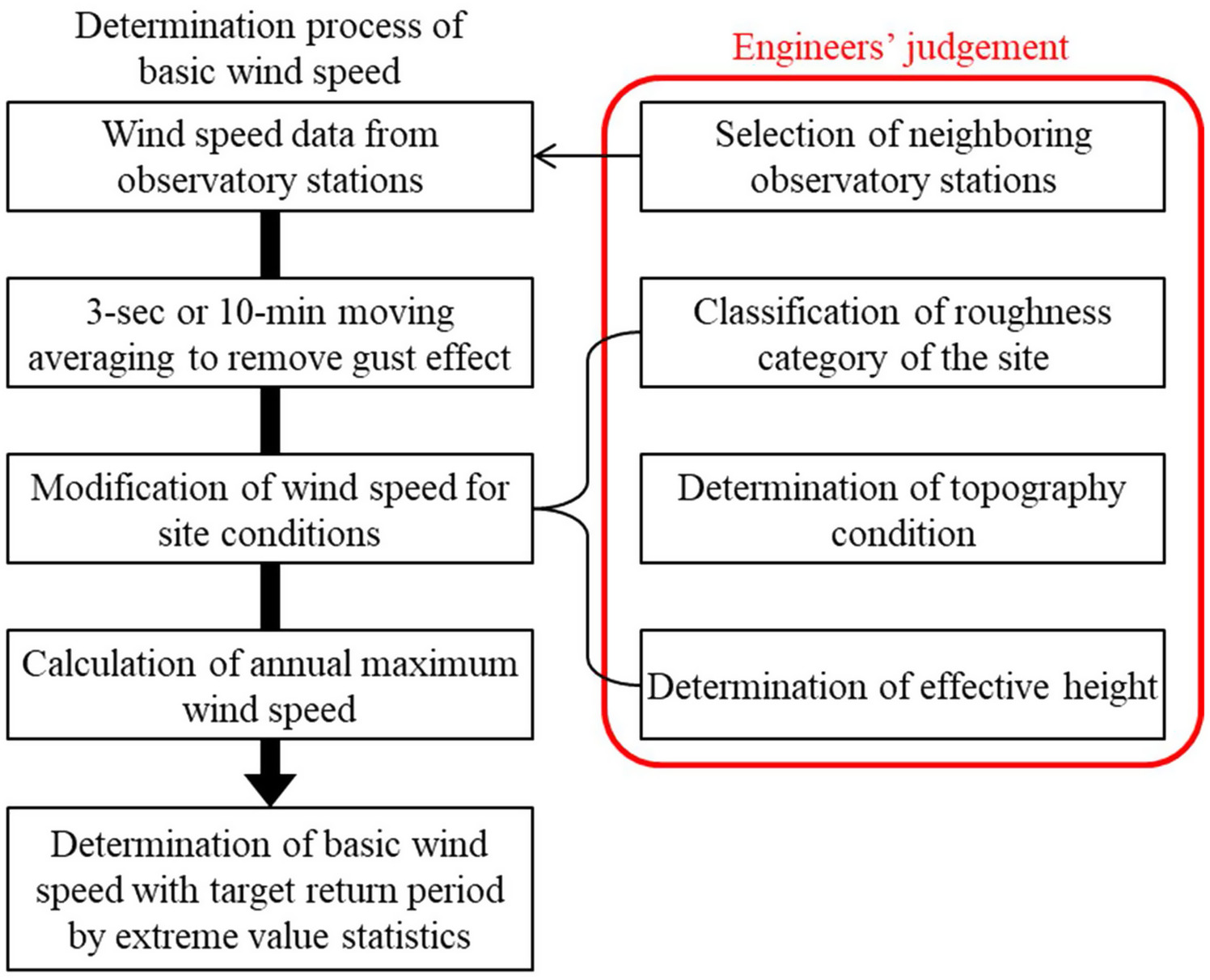
The general process for determining basic wind speed is shown in Fig. 1. Modification of wind speed for site conditions is essential. Although it is desirable to build observation stations at locations not influenced by surface roughness and topography, inevitable mountainous areas and cities conjoined with tall buildings need to be addressed. For these cases, engineering judgment is used in determination of classification, and wind speeds are modified based on empirical equations for roughness categories.
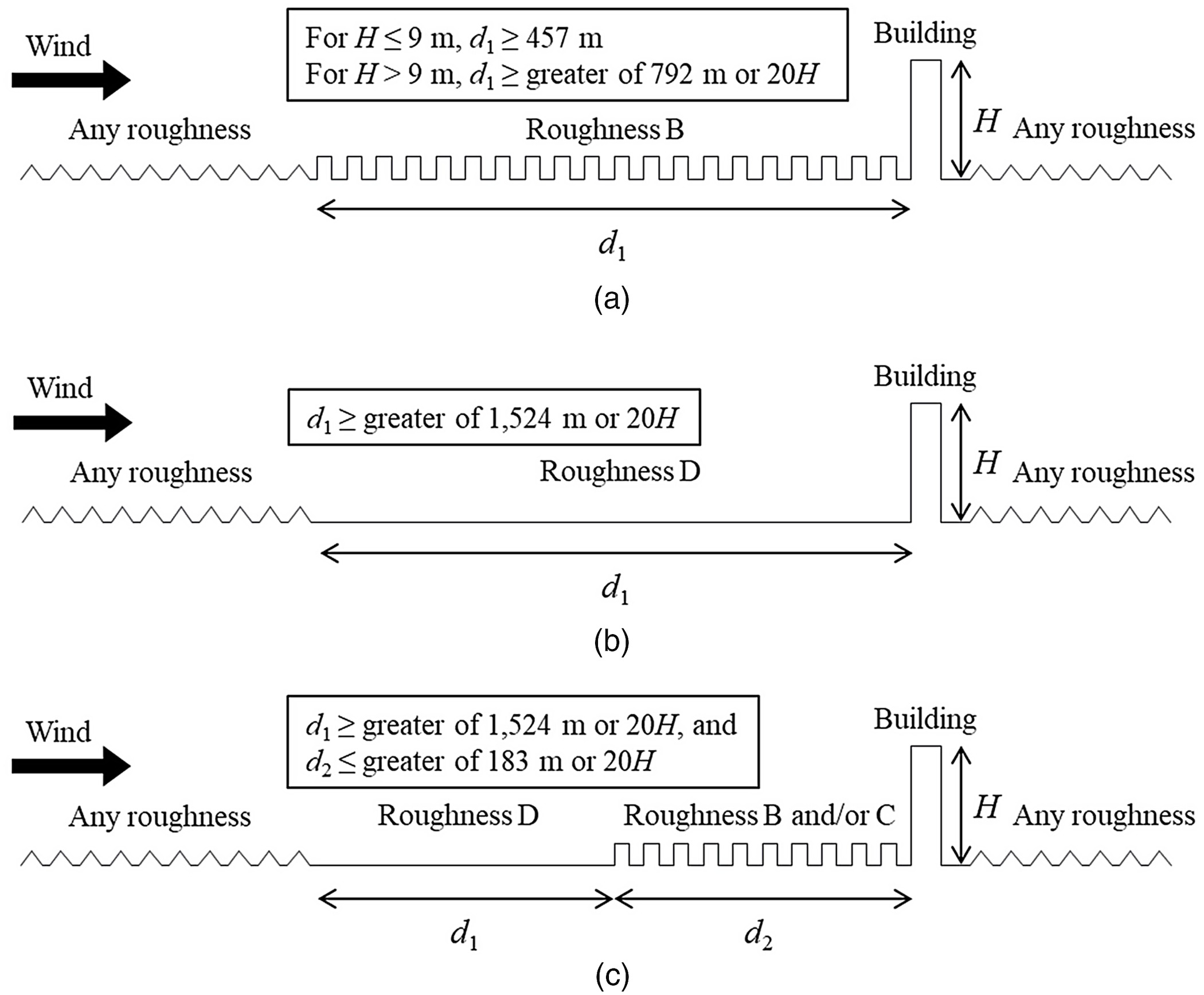
In the Commentary of ASCE 7-22, schematic explanations of combined conditions of roughness categories were presented as shown in Fig. 2. However, the spatial length conditions provided are strict and do not necessarily represent real-world circumstances. Roughness conditions in the real-world can vary with azimuth and distance. In the Commentary of Korean Building Code [KBC 2016 (MOLIT 2016)] (previous version of KDS 41:2019), roughness categories are determined from a 45° fanwise upwind surface up to or 3 km. If roughness conditions are combined, the conservative design would require the utilization of a smoother surface roughness category.
In addition to surrounding surface effects, the site height of observatory stations needs also to be considered given that hills or escarpments may increase wind speed. Design codes and standards typically employ a topography factor to account for these effects. However, difficulty exists in applied determination because the land may be too wide, continuous, and complicated. As a result, wind speed modification by an effective height was used in KDS 41:2019 based on research conducted by Jeong et al. (2014). Effective height is defined by the following equation:where = height from sea level of observatory station; = mean height from sea level to surrounding area; = mean height of buildings in surrounding area; = roughness length; and = Karman constant ≒ 0.4.
(1)
Wind speed roughness categories can be converted to that of roughness Category C (flat open terrain) using effective height and the wind speed profile factor . By definition, a wind speed profile is the ratio of wind speed at target height and target roughness to wind speed at 10 m height and roughness Category C. Wind speed above the atmospheric boundary layer is assumed to be unaffected and constant regardless of surface roughness. Thus, observed wind speed at an effective height can be converted to wind speed at 10 m height and roughness Category C, per equation . Derivation was provided by Jeong et al. (2014)where = wind speed at effective height; and = gradient height.
(2)
ASCE 7-22 and KDS 41:2019 classify the surface roughness into four categories of A to D, and the description for each category is similar (recently, ASCE has excluded Category A). However, unlike KDS, which uses a 10-min average wind speed, the ASCE method is based on a 3-s gust (or 3-s average) wind speed, and thus it is difficult to apply Eq. (2) itself. Therefore, the preceding equation for 10-min average wind speed should be converted to 3-s gust wind speed. Although there is much research regarding the relationship between the 3-s gust and 10-min average wind speed, it is reasonable to refer to Kim and Ha (2015), who proposed a gust factor that converts the 10-min average wind speed to 3-s gust wind speed because Kim and Ha (2015) used the same database of the Korea Meteorological Administration (KMA).
In this paper, the gust factor was proposed based on wind speed data observed throughout the Korean peninsula for 40 years, and the factor on surface roughness Category C as shown in Eq. (3). Therefore, according to ASCE, the wind speed at 10 m above the ground at the surface roughness Category C can be calculated by multiplying by calculated in Eq. (3)where = gust factor suggested by Kim and Ha (2015); and and gust and 10-min averaged wind speed, respectively.
(3)
After wind speed modification, basic wind speed is calculated by extreme value statistics for the target return period. KDS 41:2019 and AIJ (2015) (and many other countries’ codes) use a 100-year return period for basic wind speed, whereas ASCE 7-22 uses a 300- to 3,000-year return period depending on the risk category.
To determine an expected maximum wind speed for a period larger than the observed duration, i.e., return period, value analysis is required. The basic wind speed for a target return period is estimated from an interrelated distribution model after data fitting. Basic wind speeds in KDS 41:2019 and AIJ (2015) were determined based on a Gumbel distribution. The basic wind speed of nonhurricane and hurricane regions in ASCE 7-22 was determined by the peaks-over-thresholds (POT) model and Monte Carlo simulation, respectively.
Limitation of Engineers’ Judgment Method
As presented in Fig. 1, processes require engineering judgment. The first lies in the selection of reference stations. Research results conducted by Lee et al. (2022) revealed large potential error in estimation of basic wind speed when using one reference observation station. With an increase in the number of neighboring reference stations up to 15, estimation results improved. For accurate estimation, selection criteria for neighboring stations and fitting number of reference stations are crucial. For two or more reference stations, weighting of data from each may also be fitting.
Engineering judgment in the selection of surface roughness category classification is second. Because terrain features in the real world are very complex, classification criteria in design codes and standards cannot be applied precisely. In addition, errors in modification of wind speeds for sites with ambiguous surface conditions can be amplified for wind speed profile factors depending on roughness category.
Lastly, the topography factor used in the empirical equation based on engineering judgment is not applicable to continuous and complex topography. Modification of effective height by Jeong et al. (2014) required incorporation of elevation information for buildings and topography.
Although the process in determination of basic wind speed is well-established, many uncertainties exist. These uncertainties may be small, but accumulation and compilation of errors may be significant. Using traditional methods and engineering judgment, Lee et al. (2022) compared the 100-year return period basic wind speed at observation stations with that estimated using neighboring station data in Korea. The mean error in estimation of basic wind speed when using one reference observation station was . Given average basic wind speed in Korea is for a 100-year return period, the error attributed to use of traditional methods and engineering judgment may be very large.
Immanent in observed wind speeds are the combined effects of topography, surrounding surface roughness, and climate characteristics. It is difficult to separate these effects by human perception alone. Thus, a machine learning–based method that considers overall terrain effects on wind speeds is proposed.
Machine Learning–Based Method for Wind Speed Estimation
Built on artificial neural networks, machine learning tools have developed rapidly for various reasons, such as data growth and hardware development. In addition to structured data used for images and natural languages, it has been applied to unstructured data such as graphs. This paper briefly explains machine learning methods that may be applied in the wind speed estimation process.
Latent Model of Satellite Images
In general, the information contained in images is very large, meaning that the aforementioned “information” can be interpreted as possible cases of expression that can be expressed as a specific variable. Where in the case of general images, 256 cases can be expressed as pixels (in a black and white image, 0 means black and 255 means white). However, all information on an image, in general, is not required to recognize semblance or tasks downstream. Only abstract information or specific data are needed for downstream tasks. The latent model is an expression method of expressing high-dimensional data with some of these low-dimensional features.
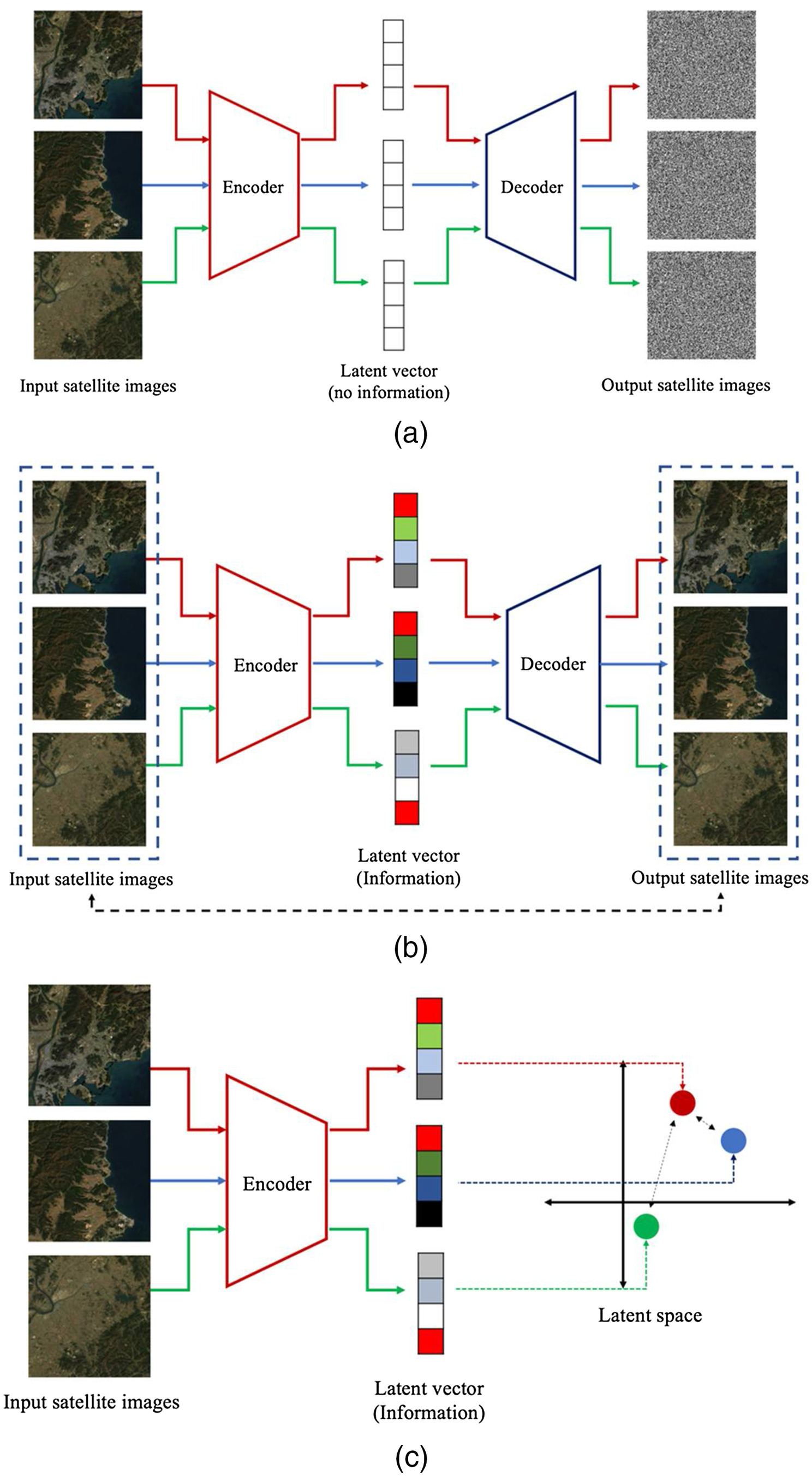
For this study, the latent model was used in the quantitative evaluation process of satellite images. As aforementioned, difficulties exist in quantitative evaluation of terrain using the existing wind speed estimation process due to degree of superfluous information present. As a result, the latent vector of the learned artificial neural network was employed for quantitative evaluation of terrain and similarity between them. The process is illustrated in Fig. 3, where before modeling is learned, there is no specific information in the latent vector and the decoding result is noise [Fig. 3(a)]. Then, the model is learned as the original image restoration; in the learning process, the latent vector numerically reflects terrain features [Fig. 3(b)]. Third, quantitative evaluation of satellite images is carried out and the relative similarity is determined in learned latent space [Fig. 3(c)].
For this paper, a quantitative evaluation of terrain was conducted using this process. There are various methods for machine learning-based latent models. Here, a variational autoencoder (VAE)–based method was used (Kingma and Welling 2014).
Transfer Learning for Efficient Satellite Feature Learning
Machine learning based on artificial neural networks has currently achieved excellent performance but requires a large amount of data, in particular, end-to-end models. Models, in general as structures become more complex, have limitations and require time to learn with increased data. These limitations may be addressed in many ways, of which transfer learning is a simple and frequently used technique. In general, information learned by the model varies depending on task, but information learned in the shallow part of the model is not very different (Zeiler and Fergus 2014). Therefore, some of the learned parameters of the learned model can be taken with additional learning performed according to the task, which is called transfer learning. Using transfer learning, less time and data are required to achieve efficient learning. Self-supervised learning may be employed for transfer learning. Recently, many studies on this aspect have been conducted through contrastive learning (Chen et al. 2018; He et al. 2020).
For this study, satellite images of a specific area and wind speed records tied thereto were required. However, unlike satellite imagery readily available, the number of observed wind speed data was limited.
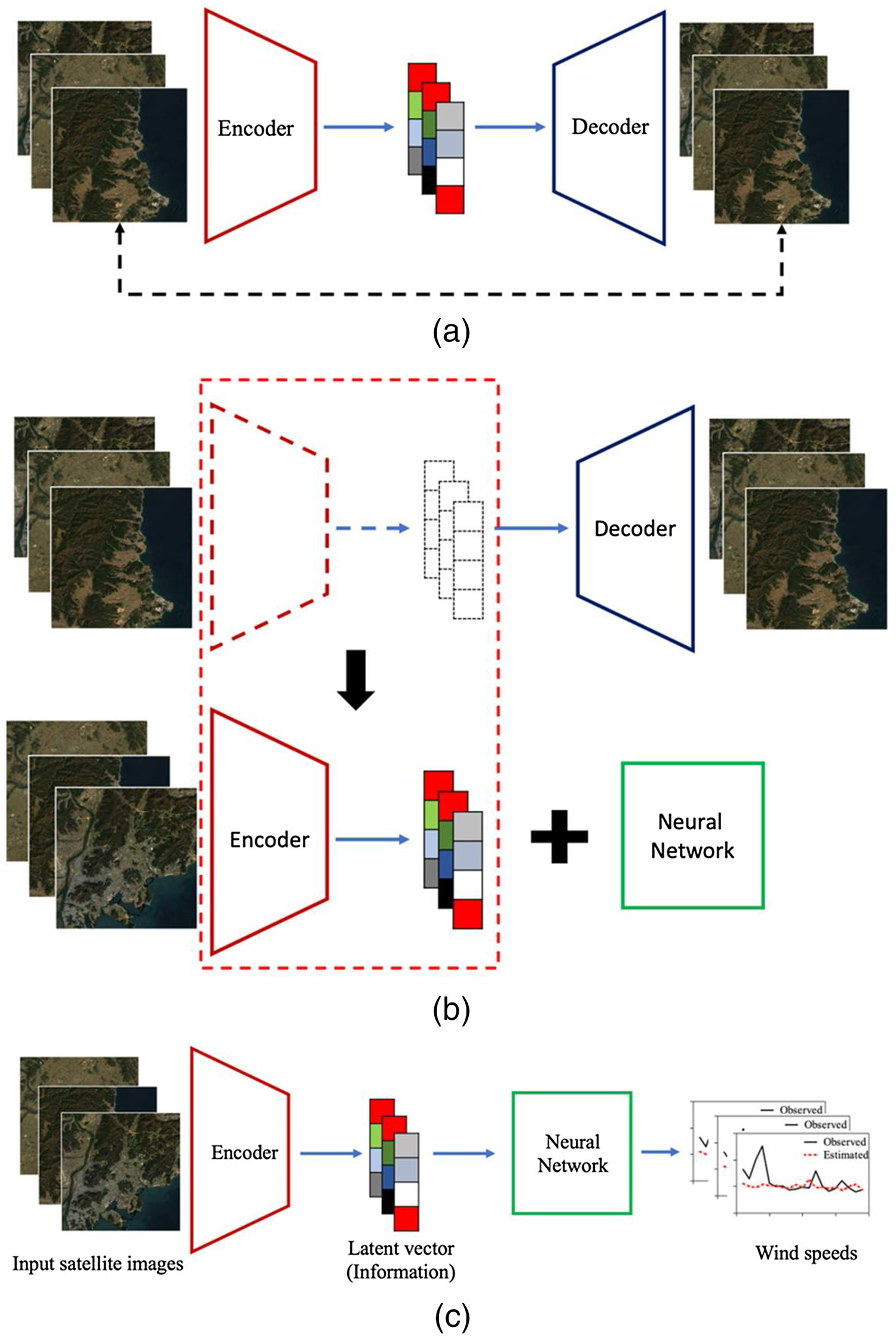
Features of the terrain are first learned from arbitrary satellite images and then transferred for use in the wind speed estimation process. This process is shown in Fig. 4. In the first stage [Fig. 4(a)] wind speed data are not required, so arbitrary satellite images may be used for latent model learning. Transferring only the encoder part of the previously learned model may be combined with an additional model that estimates wind speed [Fig. 4(b)]. Then, through satellite images and wind speed, wind speed estimation model data may be learned [Fig. 4(c)].
Graph Neural Network
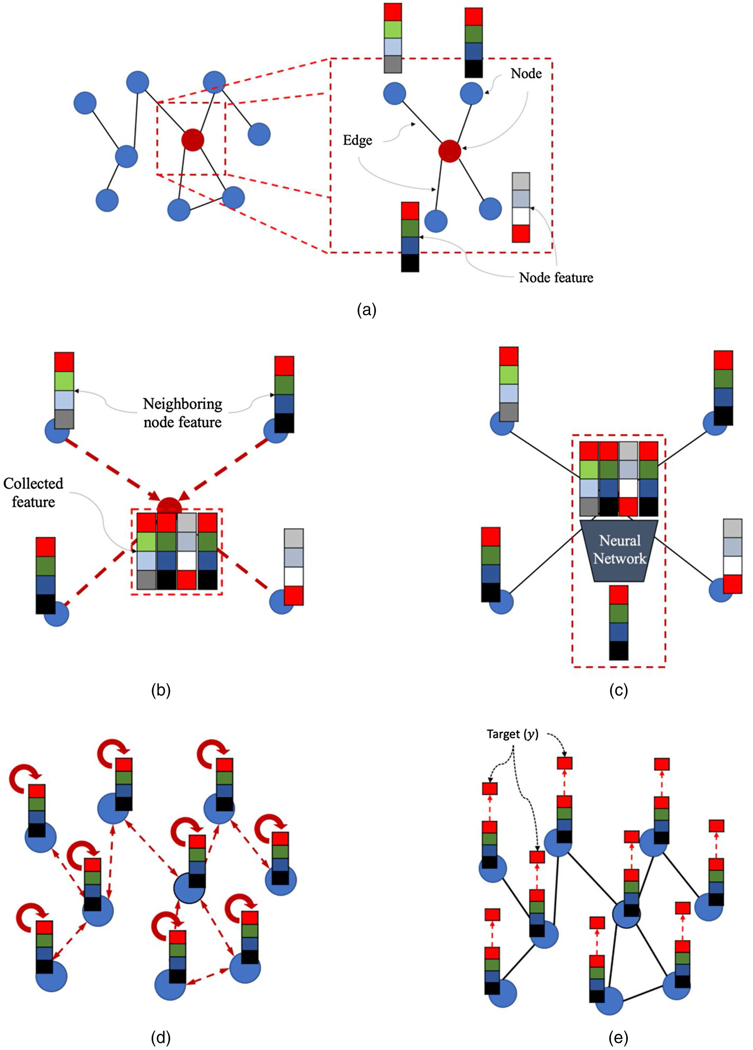
Existing machine learning based on artificial neural networks has been mainly studied in structured domains such as images and natural language. Difficulties arose in applying machine learning to unstructured data that did not have a fixed shape, such as molecular structure or social network service (SNS) network. GNN is an artificial neural network that can be applied to unstructured data (Kipf and Welling 2017). GNN operation and learning method are shown in Fig. 5. The graph consists of nodes and edges connecting nodes. Each node represents data and has a feature of that data in vector form [Fig. 5(a)]. The goal of GNN is to predict the target () through the feature of each node, and for this purpose, the node feature needs to be updated. The first step requires collection of connected neighboring node features to the corresponding node by edge [Fig. 5(b)]. Then, the collected features to a new node feature through the neural network are updated [Fig. 5(c)]. The process of Figs. 5(b and c) is repeated times for all nodes to obtain the final node feature. Finally, the target () is predicted through the final node feature [Fig. 5(e)].
GNN can be classified via several criteria. Among them, it can be divided into transductive and inductive learning. The transductive learning uses the target value of the neighboring training node when predicting the target of the test node. On the other hand, inductive learning is predicted by using only node features of all neighboring nodes.
In this study, GNN was used to express observation stations. The observation stations for the given scenario were installed irregularly in each region. A suitable means to express these stations was needed. Thus, each station was expressed as a node, and the connection between stations within a certain distance by an edge. In addition, the transductive learning was used in consideration of the relatively small amount of accumulated data.
Proposed Wind Speed Estimation Machine Learning Model
Experimental Environment
Similar to Lee et al. (2022), this study was conducted using observed wind speed data from the KMA. The KMA began meteorological observation in 1904 and has established a total of 613 observation stations [103 stations of automated synoptic observing system (ASOS) and 510 stations of automatic weather system (AWS)] to measure real-time meteorological data. As the number of years for observed wind speed data increases, the higher the accuracy of the prediction results is expected. However, the number of stations having sufficiently long observation periods was not enough. Therefore, in this study, wind speed data from stations that satisfied the following three conditions were used for training: (1) stations with 19 recent years of observation period; (2) stations whose location had not been moved more than 5 km during the observation period; and (3) stations with an effective height of 10 m. Lee et al. (2022) selected a total of 318 stations with observation period of 20 years, but it was determined that a larger number of stations were needed for better prediction performance. Thus, the target observation period was reduced to 19 years to select more stations, and a total of 341 stations were selected.
The KMA provides 1-min average wind speed data at each station, and there were several short-term missing data due to malfunction of measurement or blackout. To supplement these short-term missing data, linear interpolation was used. Based on the 1-min average wind speed data for each station, the 10-min moving averaged wind speed was calculated, and the annual maximum wind speed was calculated and used as training data.
After calculating the annual maximum wind speed for each station, some of the observed data were blind and used as validation data in order to objectively evaluate the model. The accuracy of the model was estimated in comparison with observed data, which was blinded. As a result, about 10% of total wind speed data (from 34 stations) were blinded randomly with the wind speed of the corresponding region estimated using the training data.
Two-Stage Wind Speed Estimation Model
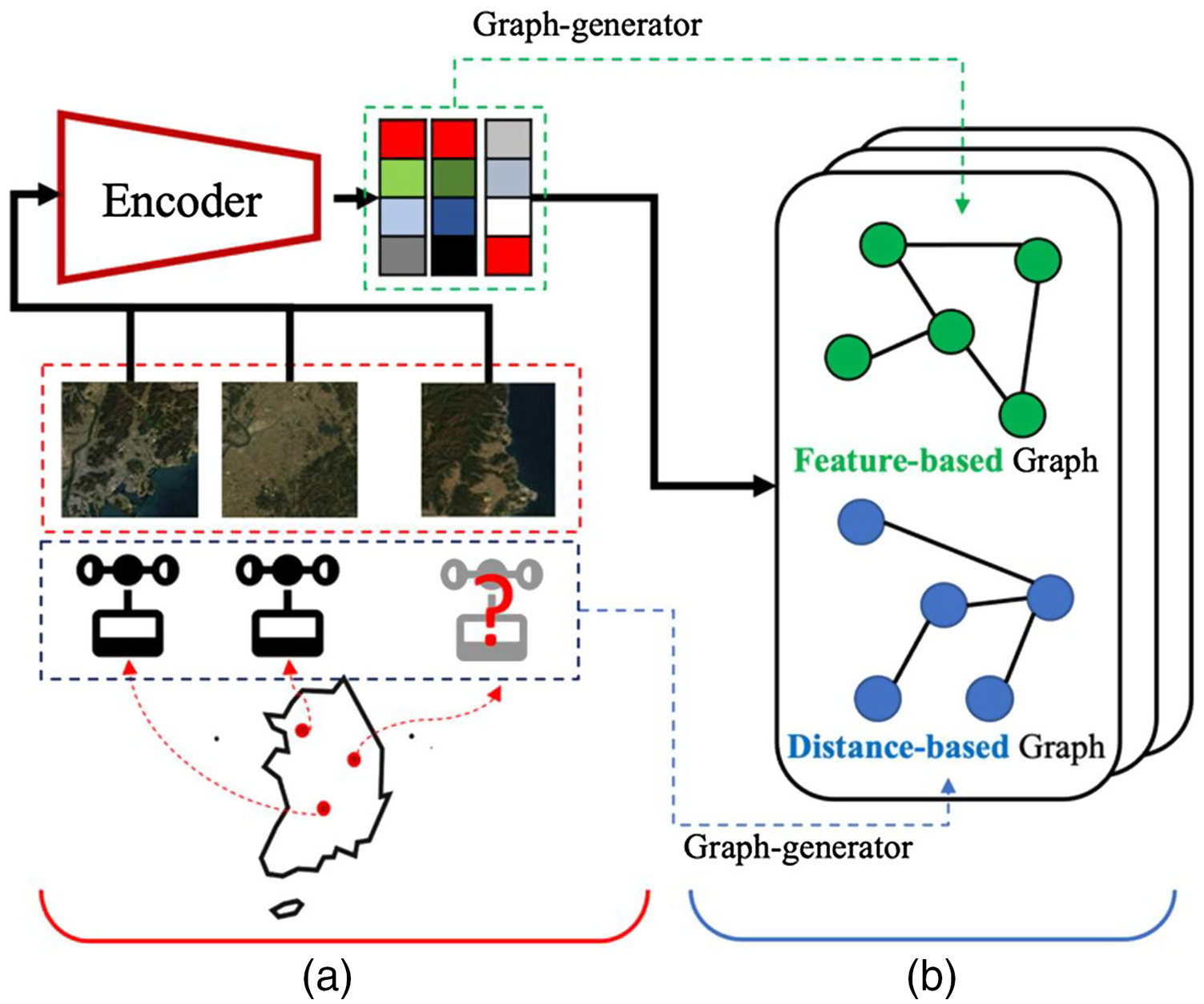
In this section, an end-to-end model that estimates wind speed using methods covered in the “Machine Learning-Based Method for Wind Speed Estimation” section is proposed. The overall structure of the model is shown in Fig. 6 and is largely comprised of two parts: the process of obtaining a latent vector from a satellite image [Fig. 6(a)]; and the process of generating two types of graphs and learning through GNN in consideration of the extracted features and location of the observation station [Fig. 6(b)].
Feature Extraction Stage
The purpose of the feature extraction stage is to obtain a latent vector of satellite images around observation stations. The encoder model, which extracts the latent vector, needs to learn features of the terrain from satellite images. The encoder part of the beta-total correlation-variational autoencoder (Beta-TC-VAE) (Chen et al. 2018) was learned using arbitrary satellite images that were transferred and used.
Wind Speed Estimation Stage
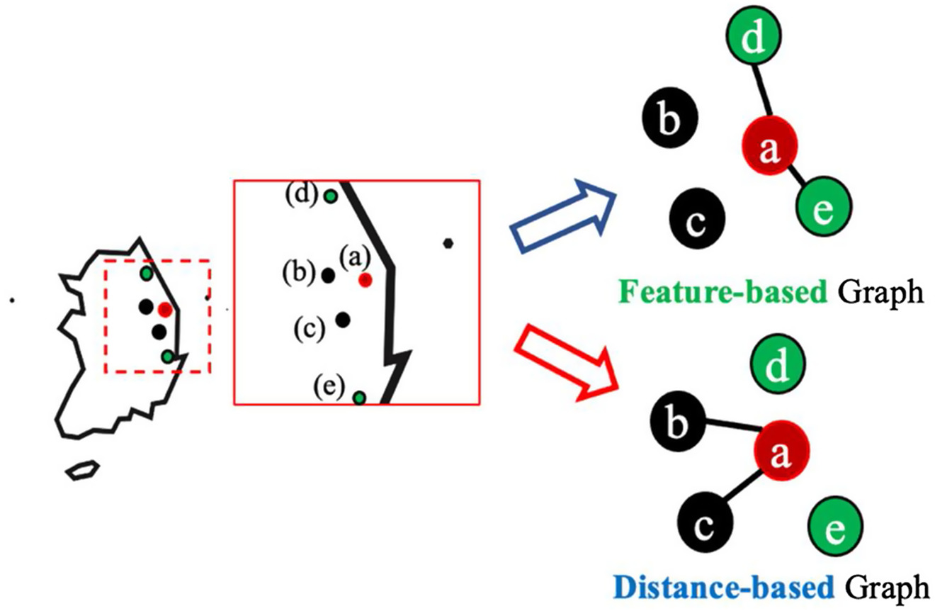
In order to learn through GNN, stations must be expressed in graph form. It was assumed that the wind speed of a specific area is simultaneously affected by two factors: (1) unique features of the area; and (2) topography features unrelated to the area. Thus, graphs based on the location of the station and graphs based on similarity of the latent vector of the topography were created and referred to as distance-based graphs and feature-based graphs, respectively. Fig. 7 provides a simple example. There are five stations (Stations ). To predict wind speed for the Area , observed data of four stations can be referenced. Whereas Stations and are relatively close in location, Stations and are relatively far away but have similar topography to Station (coastal). Thus, feature-based graphs and distance-based graphs were generated so that information for both could be used.
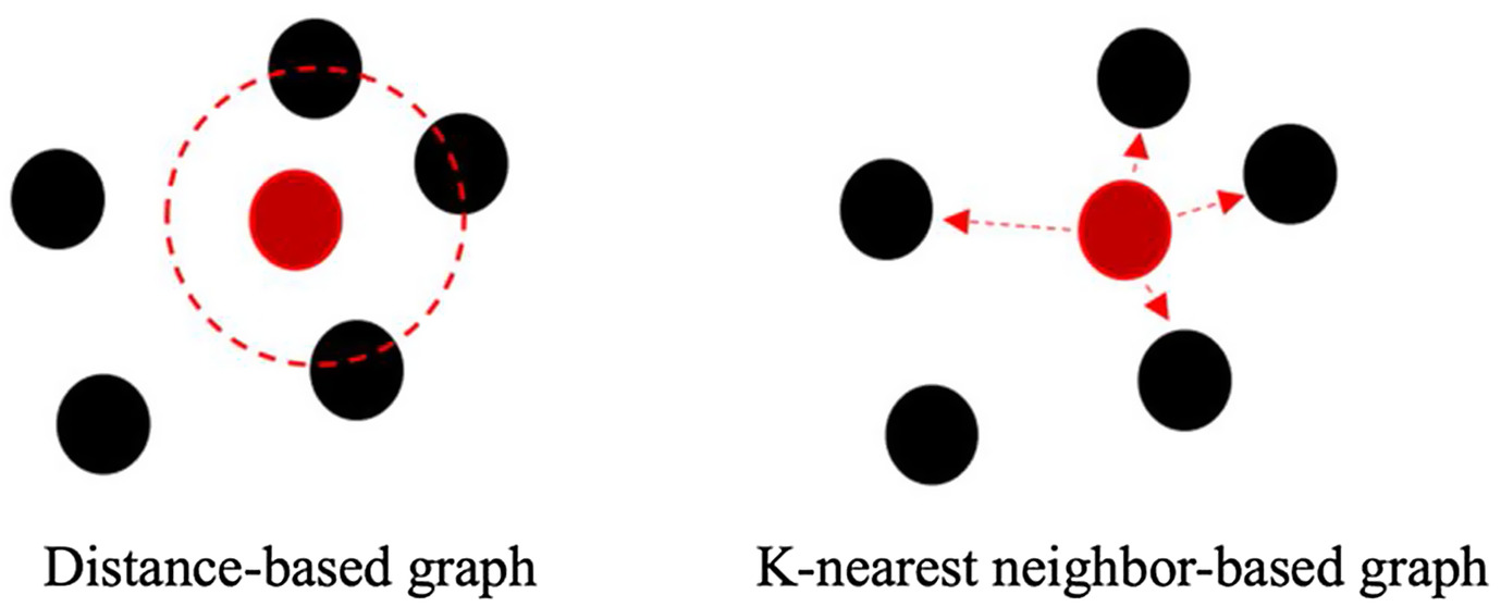
The feature-based graphs, based on the Euclidean distance between the latent vectors, generate a graph, and the distance-based graph is generated based on position of the station (Fig. 8).
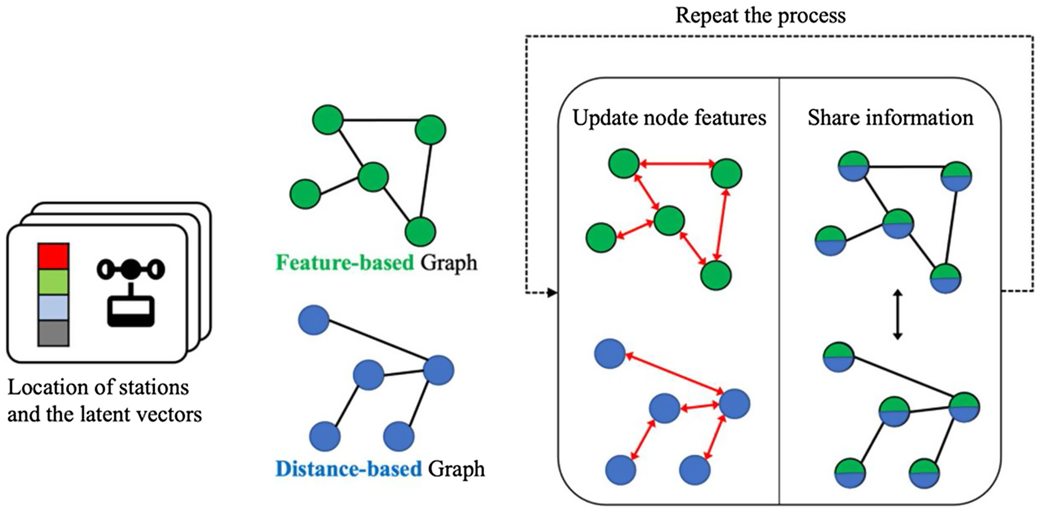
The graph generating method (Fig. 9) illustrates how GNN operates. Each graph was generated using the location of station and the latent vector obtained from the feature extraction process. Thereafter, the node feature was updated in each graph. After updating, the two graphs concatenate each feature to share information. This process was repeated based on the number of layers to obtain the final node feature. Finally, the wind speed was estimated using MLP. In this experiment, graph attention network (GATv2) (Brody et al. 2022) was used for the GNN layer. GATv2 reflects feature similarity between nodes using attention mechanism (Vaswani et al. 2017).
Analysis and Discussion of Experimental Results
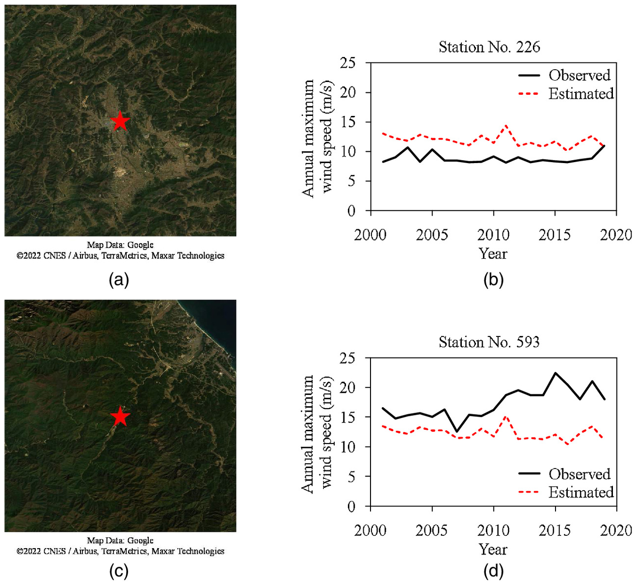
Fig. 10 compares model prediction results of several test stations with observed wind speed records. By observation, 19 years of wind speed records were estimated fairly well. The model for the 34 test stations had a mean square error (MSE) of and standard deviation of . In case of the past results using the MLP method, which were presented by Lee et al. (2022), the MSE and standard deviation were 2.917 and , respectively. Because the MSE and standard deviation of error of Lee et al. (2022) were calculated based on the prediction error of total of 318 stations, it can be considered that it was larger than that in this study calculated based on prediction error of 34 stations only. However, Lee et al. (2022) also presented an average of the error excluding 20 stations that showed the largest error, and it was . Although the number of samples was small, excluding the stations with the largest error, the average error predicted through the model presented in this study was much smaller. Therefore, it is found that the performance of the current model shows improved results compared with the previous one.
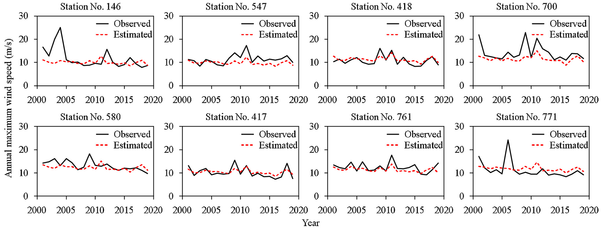
The fact that the peak value is not matched that well also needs to be pointed out as a drawback of the model. Proposal of a factor to consider outliers can be additionally considered as a further study, because the gap is consistent as well. Because data mining predicts based on existing data, it is not possible to estimate the extreme value very well due to its characteristics.
Fig. 11 shows the histogram of errors by test station and average of errors by year. In Fig. 11(a), 64% of stations depicted errors less than , with 91% less than . There was only one station with a corresponding large error exceeding . In Fig. 11(b), the average of errors observed by year was relatively high in 2003 and 2012. The error may be attributed to special environmental factors for those years, bearing need for further investigation.
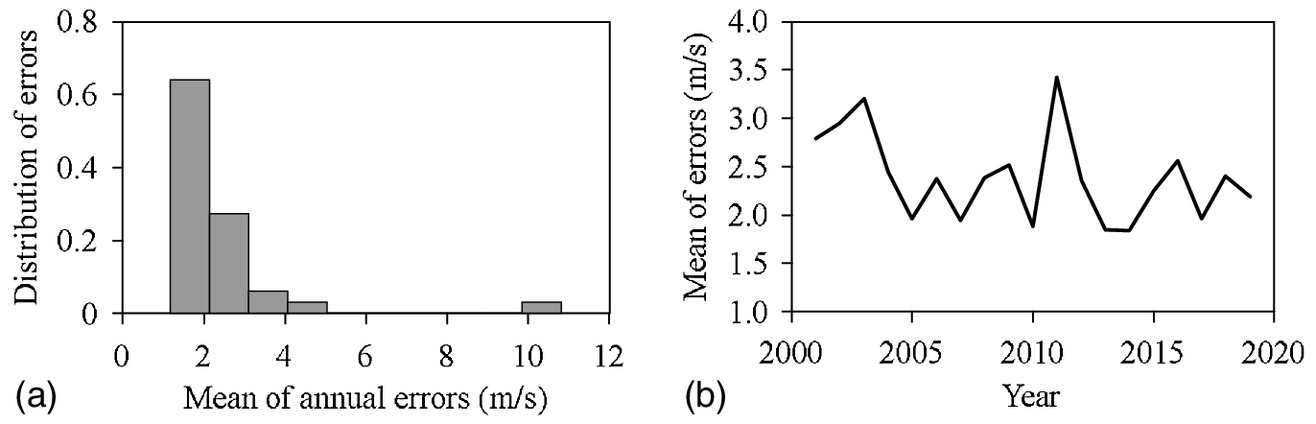
Fig. 12 shows satellite images and wind speed data of Station 185. The observed wind speed, depicted in Fig. 12(b), was 20 to , which is very large and difficult to grasp. Therefore, it is reasonable to predict errors in the observer or loss of data when compared among the 34 test stations.
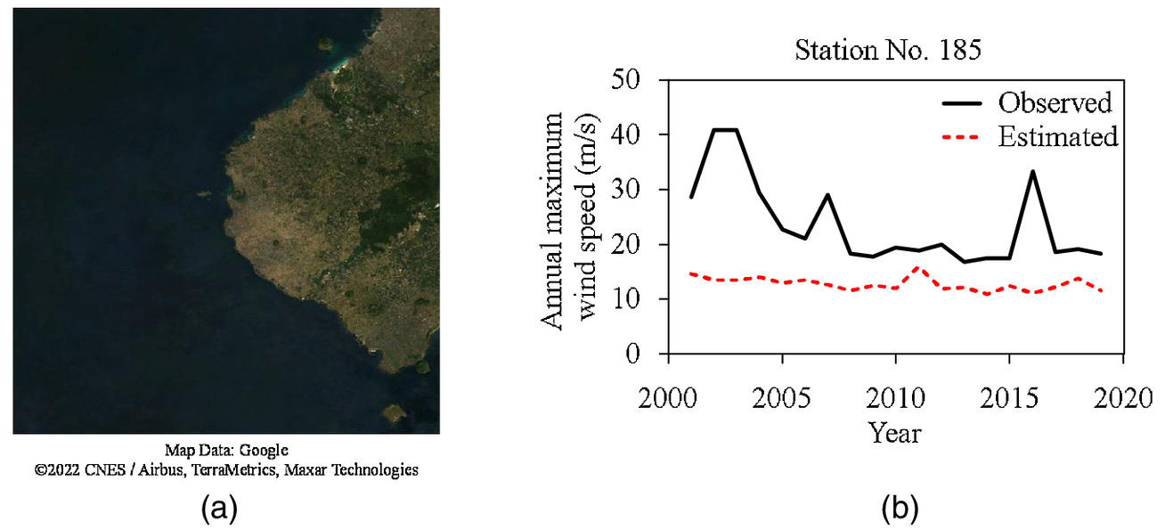
Fig. 13 shows satellite images along with observed and estimated wind speed for two regions having large errors. Specifically, terrain features such as forests when compared with other regions were not noticeable in the satellite images. Given the proposed model is a means of estimating wind speed of a region by extracting terrain features, the performance was presumed to be degraded. In the case of these two regions, further research was reckoned warranted.
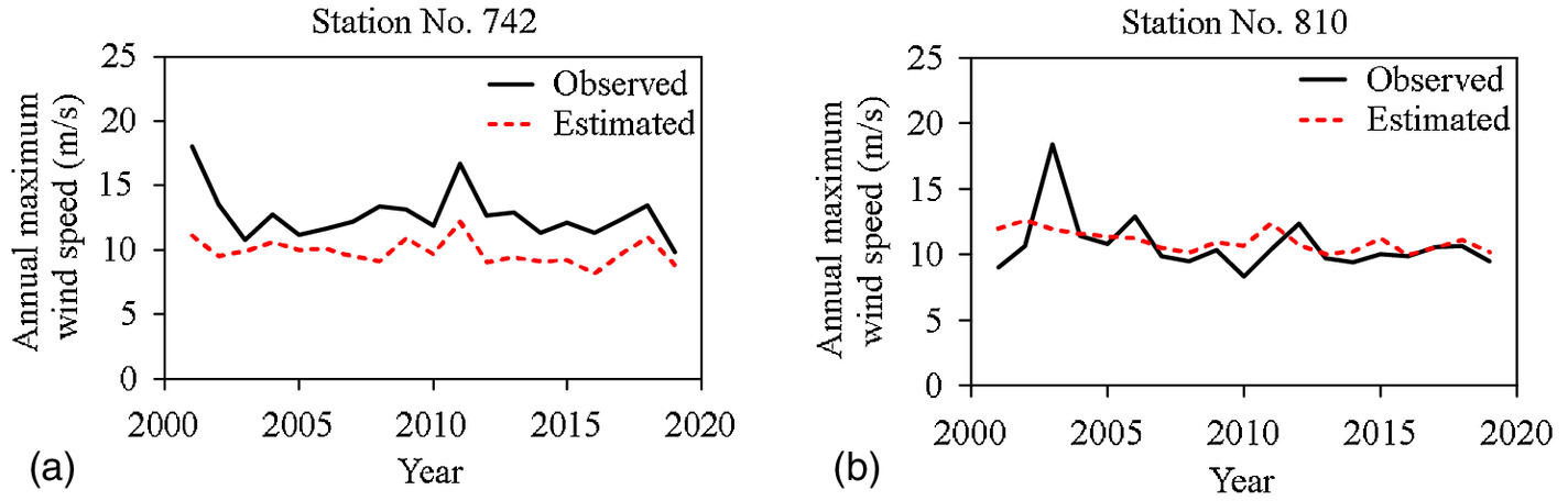
The wind speed pattern in Fig. 14 matched well, but there was indication of an ongoing slight error. In this regard, pattern information was sufficiently received, but judged not to be well aligned with the region. Although the proposed model structurally does not separate types of information, a more efficient model may result if learning were supplemented by separating absolute value and pattern of wind speed. Further research was regarded as needed. Again, it is noted that both the predicted and observed wind data included the combined effects of topography, surrounding surface roughness, and climate characteristics, and in order to determine the basic wind speed of the site, the effects of topography and surface category need to be removed or modified.
Conclusion
In this study, a machine learning method was proposed to estimate annual maximum wind speed of a specific area using observed wind speed data of surrounding observation stations. Wind speed is a basic factor in wind load design, but is difficult to estimate due to diverse and abstract factors that may affect it. In particular, the characteristics of the terrain have an important influence on wind speed. But due to the difficulty of quantitative evaluation of terrain, it has relied on qualitative evaluation by engineers. This study proposes a machine learning model that can supplement engineering evaluation. The main features of the proposed model are as follows: (1) utilization of satellite images to learn terrain characteristics; (2) utilization of GNN to express relationship between stations; and (3) use of graphs for both terrain information and location information.
The validity of the proposed model was confirmed in an experiment using Korean wind speed observation records. A case study was conducted based on experimental results, and necessity of further research and supplementation as noted confirmed:
•
The proposed model extracts and utilizes terrain features from satellite images. Without clear topographic imagery, the accuracy of the model becomes degraded. In this regard, further research is deemed warranted with potential use of other information than satellite imagery or selection of specific information from said satellite images.
•
In the experimental results, the pattern of the wind speed was fittingly estimated, but a constant error occurred steadily in some case. To this end, information related to the wind speed pattern was well learned at neighboring stations, but the information that aligns it according to the region was judged not well preserved. Although the proposed model does not structurally distinguish between these two types of information, further research on a supplemented model would need to be addressed.
Data Availability Statement
All data, models, and code generated or used during the study appear in the published article.
Acknowledgments
This work was supported by the National Foundation of Korea (NRF-2021R1A5A1032433), the Ministry of Trade, Industry & Energy of Korea (20020795), and the Institute of Engineering Research of Seoul National University. The views expressed are those of the authors, and do not necessarily represent those of the sponsors.
References
Abdi, D. S., and G. T. Bitsuamlak. 2014. “Numerical evaluation of the effect of multiple roughness changes.” Wind Struct. 19 (6): 585–601. https://doi.org/10.12989/was.2014.19.6.585.
AIJ (Architectural Institute of Japan). 2015. AIJ recommendations for loads on buildings. Tokyo: AIJ.
Alinejad, H., and T. H.-K. Kang. 2020. “Engineering review of ASCE 7-16 wind-load provisions and wind effect on tall concrete-frame buildings.” J. Struct. Eng. 146 (5): 04020100. https://doi.org/10.1061/(ASCE)ST.1943-541X.0002622.
Almaawali, S. S. S., T. A. Majid, and A. S. Yahya. 2008. “Determination of basic wind speed for building structures in Oman.” In Proc., Int. Conf. on Construction Building Tech. Selangor, Malaysia: Universiti Tenaga Nasional.
ASCE. 2022. Minimum design loads and associated criteria for buildings and other structures. ASCE 7-22. Reston, VA: ASCE.
Bahmani, P., J. van de Lindt, and T. N. Dao. 2014. “Displacement-based design of buildings with torsion: Theory and verification.” J. Struct. Eng. 140 (6): 4014020. https://doi.org/10.1061/(ASCE)ST.1943-541X.0000896.
Ballio, G., S. Lagomarsino, G. Piccardo, and G. Solari. 1999. “Probabilistic analysis of Italian extreme winds: Reference velocity and return criterion.” Wind Struct. 2 (1): 51–68. https://doi.org/10.12989/was.1999.2.1.051.
Bernardini, E., S. M. J. Spence, D.-K. Kwon, and A. Kareem. 2015. “Performance-based design of high-rise buildings for occupant comfort.” J. Struct. Eng. 141 (10): 4014244. https://doi.org/10.1061/(ASCE)ST.1943-541X.0001223.
Bowen, A. J., and D. Lindley. 1976. “A wind-tunnel investigation of the wind speed and turbulence characteristics close to the ground over various escarpment shapes.” Bound.-Layer Meteor. 12 (3): 259–271. https://doi.org/10.1007/BF00121466.
Brody, S., U. Alon, and E. Yahav. 2022. “How attentive are graph attention networks.” Preprint, submitted January 31, 2022. https://arxiv.org/abs/2105.14491.
Carpenter, P., and N. Locke. 1999. “Investigation of wind speeds over multiple two-dimensional hills.” J. Wind Eng. Ind. Aerodyn. 83 (1): 109–120. https://doi.org/10.1016/S0167-6105(99)00065-3.
CEN (European Committee for Standardization). 2003. Actions on structures—General actions—Part 1.4: Wind actions. Eurocode 1. Brussels, Belgium: CEN.
Chen, R.-T.-Q., X. Li, R. Grosse, and D. Duvenaud. 2018. “Isolating sources of disentanglement in variational autoencoders.” In Proc., 32nd Conf. on Advances in Neural Information Processing Systems. San Diego: Neural Information Processing Systems.
Cui, W., and L. Caracoglia. 2020. “Performance-based wind engineering of tall buildings examining life-cycle downtime and multisource wind damage.” J. Struct. Eng. 146 (5): 4019179. https://doi.org/10.1061/(ASCE)ST.1943-541X.0002479.
ESDU (Engineering Sciences Data Unit). 2000. Mean wind speeds over hills and other topography (ESDU 91043). London: ESDU.
ESDU (Engineering Sciences Data Unit). 2012. Wind speed profiles over terrain with roughness changes (ESDU 84011). London: ESDU.
He, K., H. Fan, Y. Wu, S. Xie, and R. Girshick. 2020. “Momentum contrast for unsupervised visual representation learning.” In Proc., Conf. on Computer Vision and Pattern Recognition. New York: IEEE.
ISO. 2009. Wind actions on structures. ISO 4354. Geneva: ISO.
Jeong, S.-H., B.-J. Kim, and Y.-C. Ha. 2014. “Revision of basic wind speed map of KBC-2009.” [In Korean.] J. Archit. Inst. Korea Struct. Constr. 30 (5): 37–47.
Jeong, S.-Y., H. Alinejad, and T. H.-K. Kang. 2021. “Performance-Based wind design of high-rise buildings using generated time-history wind loads.” J. Struct. Eng. 147 (9): 04021134. https://doi.org/10.1061/(ASCE)ST.1943-541X.0003077.
Kang, T. H.-K., S.-Y. Jeong, and H. Alinejad. 2019. “Understanding of wind load determination according to KBC 2016 and its application to high-rise buildings.” [In Korean.] J. Wind Eng. Inst. Korea 23 (2): 83–89.
Kim, B.-J., and Y.-C. Ha. 2015. “Estimation of gust factors suitable for the surface roughness category based on the recent meteorological data in Korea.” [In Korean.] J. Wind Eng. Inst. Korea 19 (2): 51–57.
Kingma, D.-P., and M. Welling. 2014. “Auto-encoding variational Bayes.” Preprint, submitted May 1, 2014. https://arxiv.org/abs/1312.6114.
Kipf, T., and M. Welling. 2017. “Semi-supervised classification with graph convolutional networks.” Preprint, submitted February 22, 2017. https://arxiv.org/abs/1609.02907.
Koo, J., G.-D. Han, H.-J. Choi, and J.-H. Shim. 2015. “Wind-speed prediction and analysis based on geological and distance variables using an artificial neural network: A case study in South Korea.” Energy 93 (7): 1296–1302. https://doi.org/10.1016/j.energy.2015.10.026.
Kwon, D. K., S. M. J. Spence, and A. Kareem. 2015. “Performance evaluation of database-enabled design frameworks for the preliminary design of tall buildings.” J. Struct. Eng. 141 (10): 4014242. https://doi.org/10.1061/(ASCE)ST.1943-541X.0001229.
Lakshmanan, N., S. Gomathinayagam, P. Harikrishna, A. Abraham, and S. C. Ganapathi. 2009. “Basic wind speed map of India with long-term hourly wind data.” Curr. Sci. 96 (7): 911–922.
Lee, D.-H., S.-Y. Jeong, and T. H.-K. Kang. 2022. “Consideration of terrain features from satellite imagery in machine learning of basic wind speed.” Build. Environ. 213: 108866. https://doi.org/10.1016/j.buildenv.2022.108866.
Lou, W., L. Zhang, M. F. Huang, and Q. S. Li. 2015. “Multiobjective equivalent static wind loads on complex tall buildings using non-gaussian peak factors.” J. Struct. Eng. 141 (11): 4015033. https://doi.org/10.1061/(ASCE)ST.1943-541X.0001277.
MOLIT (Ministry of Land, Infrastructure and Transport). 2016. Korean building code. KBC 2016. Sejong, South Korea: MOLIT.
MOLIT (Ministry of Land, Infrastructure and Transport). 2019. Korean design standard. KDS 41:2019. Sejong, South Korea: MOLIT.
Ouyang, Z., and S. M. J. Spence. 2020. “A performance-based wind engineering framework for envelope systems of engineered buildings subject to directional wind and rain hazards.” J. Struct. Eng. 146 (5): 4020049. https://doi.org/10.1061/(ASCE)ST.1943-541X.0002568.
Tamura, Y. 2020. “Mathematical models for understanding phenomena: Vortex-induced vibrations.” Jpn. Archit. Rev. 3 (4): 398–422. https://doi.org/10.1002/2475-8876.12180.
Vaswani, A., N. Shazzer, N. Parmar, J. Uszkoreit, L. Jones, A.-N. Gomez, L. Kaiser, and L. Polosukhin. 2017. “Attention is all you need.” In Proc., 30th Conf. on Advances in Neural Information Processing Systems. San Diego: Neural Information Processing Systems.
Wang, T., S. Cao, and Y. Ge. 2014. “Effects of inflow turbulence and slope on turbulent boundary layer over two-dimensional hills.” Wind Struct. 19 (2): 219–232. https://doi.org/10.12989/was.2014.19.2.219.
Wani, A. H., R. K. Varma, and A. K. Ahuja. 2021. “Experimental investigation of wind flow characteristics over hills and escarpments—A review.” Wind Struct. 32 (4): 393–403. https://doi.org/10.12989/was.2021.32.4.393.
Zeiler, M.-D., and R. Fergus. 2014. “Visualizing and understanding convolutional networks.” In Proc., 16th European Conf. on Computer Vision. Cham, Switzerland: Springer.
Information & Authors
Information
Published In

Journal of Structural Engineering
Volume 149 • Issue 1 • January 2023
Copyright
This work is made available under the terms of the Creative Commons Attribution 4.0 International license, https://creativecommons.org/licenses/by/4.0/.
History
Received: Feb 1, 2022
Accepted: Aug 22, 2022
Published online: Nov 12, 2022
Published in print: Jan 1, 2023
Discussion open until: Apr 12, 2023
Authors
Metrics & Citations
Metrics
Citations
Download citation
If you have the appropriate software installed, you can download article citation data to the citation manager of your choice. Simply select your manager software from the list below and click Download.