Unit Operation and Process Modeling with Physics-Informed Machine Learning

Li, Haochen; Spelman, David; Sansalone, John

doi:10.1061/JOEEDU.EEENG-7467

Open access

Technical Papers

Jan 25, 2024

Unit Operation and Process Modeling with Physics-Informed Machine Learning

Authors: Haochen Li, Ph.D., M.ASCE https://orcid.org/0000-0002-2343-2813 [email protected], David Spelman, Ph.D., M.ASCE https://orcid.org/0000-0002-5214-3092 [email protected], and John Sansalone, Ph.D., M.ASCE [email protected]Author Affiliations

Publication: Journal of Environmental Engineering

Volume 150, Issue 4

https://doi.org/10.1061/JOEEDU.EEENG-7467

PDF

Abstract

Machine learning (ML) is increasingly implemented to model water infrastructure dynamics. Common ML models are primarily data-driven and require a significant amount of data for robust training. Often, obtaining robust data at higher temporal and spatial resolutions in water systems can be challenging due to cost and time considerations. In such scenarios, integrating the existing scientific knowledge into an ML model as physics-informed ML can be advantageous to enhance predictive capability and generalizability. This study examines the predictive capability and generalizability of physics-informed ML and common ML models for typical unit operation and process (UOP) system dynamics in urban water treatment. The systems studied are (1) a continuous stirred-tank reactor, (2) activated sludge reactor, and a (3) fixed-bed granular adsorption reactor. Applications of physics-informed neural networks (PINNs) are presented. Results demonstrate when the availability of data is limited: (1) common ML models are not necessarily robust for predicting water system dynamics, except when system dynamics exhibit simpler periodic patterns. Common ML models also do not generalize across different loading conditions. (2) In contrast, the developed PINN models yield high predictive capability and generalizability. (3) Benefiting from the embedded prior knowledge, PINNs require significantly reduced data sets for robust predictions. These results suggest hybridizing physics principles and domain knowledge into the ML framework can be critical for robust UOP and water systems modeling.

Introduction

Artificial intelligence (AI) and data-driven solutions are revolutionizing the modeling and prediction of complex systems (Brunton and Kutz 2019; Taoufik et al. 2022; Yu et al. 2023; Liu et al. 2023). Within AI, machine learning (ML) offers a wealth of solutions to extract information from physical and numerical data, which can be translated into knowledge and inform the dynamics and management of water systems such as the unit operation and process (UOP). In recent years, ML techniques have been increasingly applied for modeling natural and engineered water systems (Pyo et al. 2020; Valencia et al. 2021; Huang et al. 2021; Li et al. 2021a, b; Abdeldayem et al. 2022; Liu et al. 2022; Sundui et al. 2021; Trueman et al. 2022; Ly et al. 2022). Zhi et al. (2021) implemented a long short-term memory (LSTM) model for predicting dissolved oxygen in rivers at a continental scale in the United States (US). Thompson and Dickenson (2021) used ML to detect adverse water chemistry events in drinking water sources in Las Vegas, Nevada. Guo et al. (2015) applied artificial neural networks (ANN) and support vector machine (SVM) to predict total nitrogen (TN) in the effluent of a wastewater treatment plant. Zaghloul et al. (2021) developed an ensemble of ML algorithms for simulating aerobic granular sludge. Li and Sansalone (2022a) modeled particulate matter separation for urban water clarification basins with symbolic regression. Abdalla et al. (2021) simulated runoff from green roofs with different ML methods. Such research demonstrates the applicability and potential of ML for modeling urban water systems, whether for storm-, waste-, or potable water systems.

Notwithstanding the increased applications and potential benefits of common ML models, the robustness and potential liability for predicting system dynamics receive less examination. Common ML models for water system modeling are typically formulated as supervised ML problems. Given observed data, ML models are trained to forecast quantities of interest such as chemical oxygen demand (COD), biochemical oxygen demand (BOD), total phosphorus (TP), TN, and suspended sediment concentration (SSC) (Guo et al. 2015; Huang et al. 2021; Sundui et al. 2021; Viet and Jang 2023). In such common ML models based on supervised learning, three main obstacles potentially hinder their predictive capability: (1) common ML models are largely data-driven. Therefore, these models are a “black box” and are agnostic to domain knowledge (e.g., stoichiometry, reaction kinetics) and physics principles (e.g., mass, momentum, energy conversation principles) (Raissi et al. 2019; Li et al. 2022). Their predictions are not guaranteed to be physical (e.g., predict more species mass than the sum of system input species mass and system species mass generation) or even physically bounded (e.g., negative values in the predicted species concentration). (2) Common ML models for water system modeling, while different in the detailed model implementation [e.g., ANN, random forest (RF), decision tree (DT), SVM,

k

-nearest neighbors (KNN)] are commonly formulated as supervised learning (Huang et al. 2021). As demonstrated by Mallat (2016), “Supervised learning is a high-dimensional interpolation problem.” Therefore, common ML models require large and diverse data sets for model training. However, distinct from conventional applications of ML models in social networks and computer vision, data acquisition for water systems at this time is more challenging and less economical (Jia et al. 2021). Except for selected parameters monitored with online sensors in real-time (e.g., dissolved oxygen, turbidity, pressure, ammonia), basic and critical parameters still primarily rely on discrete samples and laboratory analysis such as SSC, particle size distribution, TP, TN, and metals (other inorganic and organic chemicals notwithstanding). With a limited database, training and development of a common ML can result in poor model generalizability and can be less robust (Newhart et al. 2019). (3) The prediction/forecasting of system dynamics is essentially a task of extrapolation in time. While common ML models can perform well for interpolation problems, such models can be significantly challenged by extrapolation. Moreover, generalizability is not ensured when a model is applied to different loading conditions. Considering the potential liabilities of ML and the unique challenges of limited data in urban water systems, there is a critical need to examine the predictive capability of common ML models for water system dynamics.

Building on the contributions provided by common ML models, a potentially more robust ML approach for modeling water system dynamics is scientific machine learning (SciML) (Karniadakis et al. 2021; Ghattas and Willcox 2021; Quaghebeur et al. 2022). SciML is an emerging family of ML methods that hybridizes scientific computing (e.g., differential equations, computational fluid dynamics) and ML. SciML augments common ML methods by integrating domain knowledge and physics principles (as differential equations) into ML models through novel ML architecture. In SciML, ML models reflect data-driven learning yet are not “black boxes” and are deeply embedded with prior knowledge of the underlying system physics (Ghattas and Willcox 2021). In the last few years, several SciML frameworks and ecosystems have been developed for dynamic system modeling such as universal differential equations (UDEs) (Rackauckas et al. 2020), sparse identification of nonlinear dynamics (Kaptanoglu et al. 2022), neural ordinary differential equations (neural ODEs) (Chen et al. 2018), and physics-informed neural networks (PINNs) (Raissi et al. 2019). By incorporating domain knowledge, SciML can significantly improve predictive capability and robustness compared with common ML methods. Further, SciML has also demonstrated higher efficacy for many inverse problems that challenge conventional mechanistic models (differential equations), such as model parameter estimations and discovery of hidden dynamics (Yazdani et al. 2020).

This study leverages recent advancements in SciML and presents a novel application for PINNs to common UOPs in urban water treatment, whether for storm-, waste-, or potable water treatment. The specific objectives of this study are to generalize and summarize common ML methods and models for water system modeling and to examine and compare the predictive capability of common ML and SciML models (i.e., PINNs) for common UOPs: (1) a CSTR; (2) an activated sludge reactor; (3) a fixed bed adsorption reactor; and assess the capability of PINNs for parameter estimation with partial observation data.

Materials and Methods

As a framework of materials and methods, common ML models for modeling water system dynamics are generalized and summarized in subsection “Common machine learning models.” Subsection “Physics-informed neural networks for UOPs” introduces PINNs for water system modeling. Subsection “Cases examined” illustrates the three UOP systems (CSTR, activated sludge reactor, and fixed-bed adsorption reactor), which are tested to examine common ML models and PINNs. The methodology and implementation of PINNs for each case are also detailed.

Common Machine Learning Models

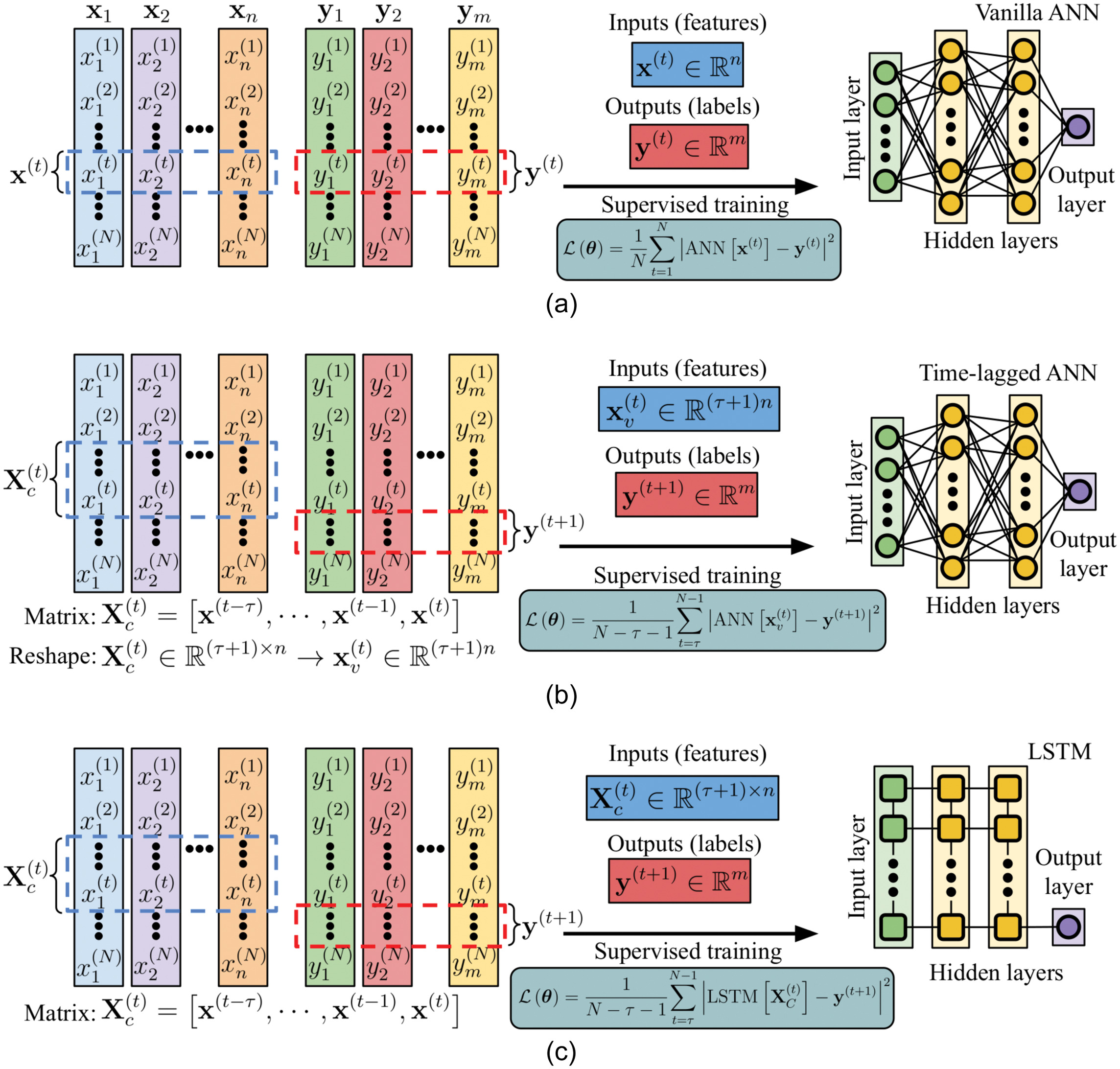
Common ML models for water system dynamics modeling (often as time series), while differing in the detailed implementation and specific ML model applied (e.g., ANN, RF, DT, SVM, KNN), are formulated as a supervised ML problem. Such models can be categorized into the three methods as listed here. Fig. 1 illustrates the data layout, supervised training formulation, and model structure of these methods with ANN and LSTM. ANN is considered because of the high flexibility of ANN to handle multiple outputs, computational efficiency in leveraging modern graphics processing units (GPU) for large data training, and the close relationship of ANN with PINNs (introduced in the next section).

1.

Instant mapping method (Godo-Pla et al. 2019; Zhang et al. 2019; Newhart et al. 2020a). In this method, the features (e.g., flowrate, influent loads) at a current time are used as inputs to ML models

x^{(t)}

. ML models output the quantities of interest such as effluent chemistry parameters or load as labels

y^{(t)}

. ML model parameters

θ

(in the case of ANN,

θ

are the ANN weights and biases) are obtained through supervised training by minimizing the loss function

L (θ)

[i.e., mean squared error (MSE)] between the ML model prediction

ANN [x^{(t)}]

and

y^{(t)}

. With this method, water system dynamics modeling as a time-series is not significantly different from classic ML-based regression (Li and Sansalone 2022a). Time

t

in this method only serves as an index for different data pairs

[x^{(t)}, y^{(t)}]

, and shuffling the time index will not influence the model training and results, since the model label/output at a given time only depends on the model input at that time.

2.

Time-lagged mapping method (also known as the sliding window approach or recursive approach) (French et al. 1992; Recknagel et al. 1997; Wu and Lo 2008; Griffiths and Andrews 2011; Wang et al. 2021; Abdalla et al. 2021; Brunton and Kutz 2019; Newhart et al. 2020a, b). This method is developed to utilize the time-sequential information embedded in the time-series data. Sequential information can be important for prediction outcomes. For example, a higher effluent concentration at the current time is likely to associate with a higher effluent concentration in the previous time. As illustrated by Fig. 1(b), the features

X_{c}^{(t)}

(from previous times

t - τ

until the current time

t

) are used and reshaped (i.e., flattened) as ML model inputs

x_{v}^{(t)}

to predict the output label in the future time

y^{(t + 1)}

. Note that, alternatively, ML model inputs

x_{v}^{(t)}

can also include the history data of the output labels as an autoregressive component (French et al. 1992; Brunton and Kutz 2019). By such a formulation, the historical influence in the time-series is partially considered by the ML model, although the temporal ordering within the input

x_{v}^{(t)}

of each data pair is ignored (i.e., features in

x_{v}^{(t)}

at a different time is treated as independent features) (Lara-Benítez et al. 2021). The subsequent supervised training is essentially training an ML model to learn an update rule (i.e., updates the output label based on the history data) (Brunton and Kutz 2019). In contrast with the previous instant mapping method, the time

t

index ordering in the time-lagged mapping method contains sequential information and cannot be shuffled. The ML model structure used in this method, however, is not significantly different from the ML model applied in the previous instant mapping method (because this method is agnostic to the temporal ordering within the input

x_{v}^{(t)}

and treating features at a different time as independent features). Only the input layer size is expanded from

R^{n}

to

R^{(τ + 1) n}

to accommodate more features (because of considering historical features).

3.

Long-short term memory (LSTM) (Hochreiter and Schmidhuber 1997; Antanasijević et al. 2013; Pisa et al. 2019; Abdalla et al. 2021; Zhi et al. 2021; Li and Vanrolleghem 2022; Newhart et al. 2020a). As a type of recurrent neural network (RNN), LSTM is specifically developed for modeling time-dependent data. As illustrated in Fig. 1(c), LSTM combines features from the previous time and current time for prediction (indicated by the vertical connection lines between LSTM units in each layer). The temporal relationship within the input feature is considered through hidden states and cell states. Moreover, compared with vanilla RNN, LSTM overcomes the issue of a vanishing gradient in learning long-term dependencies by the novel architecture design of cell states and gating mechanisms (Hochreiter and Schmidhuber 1997). As suggested by the name, LSTM is capable of capturing long- and short-term dependencies of the data. The training data layout with LSTM adopted here is identical to the previous time-lagged mapping method. Since LSTM is often applied to predict labels at one future time instant, a stacked “many to one” LSTM structure is illustrated in Fig. 1(c).

Fig. 1. Illustration of data layout, supervised training formulation, and model structure in common ML models implemented for UOP modeling. (a) Vanilla ANN; (b) time-lagged ANN; and (c) LSTM model. $X$ and $y$ are the model inputs and outputs, $t$ is time, $R^{r \times s}$ denotes the variable is a $r$ by $s$ matrix with real numbers, $τ$ is the lagged time period, $L$ is the loss function [mean squared error (MSE)], and $N$ is total number of paired data sets. $n$ and $m$ are number of inputs and outputs. $θ$ are the ML model parameters (e.g., weights and bias in the case of ANN).

Physics-Informed Neural Networks for UOPs

In contrast with common ML models, SciML hybridizes physics principles and domain knowledge with data. Specifically, PINNs introduced by Raissi et al. (2019) integrate the prior domain knowledge into ANN by posing constraints on the loss function in ANN training. Other SciML approaches such as neural ODEs (Chen et al. 2018) have been recently adopted (Quaghebeur et al. 2022). Herein, the PINNs implementation directly facilitates integration for ODE and PDE systems (or mixed PDE-ODE systems). The capability of accommodating PDEs is necessary for modeling time-varying and spatially dependent water systems (demonstrated in the later section). Fig. 2 illustrates the proposed PINNs for common UOPs in urban water treatment. The implementation of PINNs depends on the specific system, which is detailed for each UOP case examined in subsection “Cases examined.” The general elements and key concepts of PINNs methodology are as follows:

1.

System dynamics can be represented by state variables

Y

(e.g., species concentration, turbidity, SSC, etc.). Depending on the specific system, the system state variables

Y

can be a function of space

Y (X)

(i.e., time-independent spatially varying system), a function of time

Y (t)

(i.e., unsteady spatially uniform system), or a function of space and time

Y (t, X)

(i.e., time-dependent spatially varying system).

2.

Based on a universal approximation theorem, the ANN is applied to model the system state variables

Y (t, X) = ANN (t, X)

. Here, a time-dependent spatially varying system is considered for illustration. In the ANN formulation, the time

t

and space coordinates

X = (x, y, z)

are the input features and ANN outputs the system state variables

Y

. Given observation data of state variables (i.e., labels), a supervised ML problem can be formulated, and ANN can be trained to predict the state variables

Y

based on inputs

(t, X)

, as shown in Eq. (1). This data-driven part of PINNs is identical to the vanilla ANN model illustrated in Fig. 1(a)

L^{data} (θ) = \frac{1}{N_{d}} \sum_{i = 1}^{N_{d}} {| ANN [t^{(i)}, X^{(i)}] - y^{(i)} |}^{2}

(1)

In this equation,

L^{data}

= the data loss function (i.e., MSE) in PINNs;

θ

= the ANN model parameters (i.e., weights and biases);

N_{d}

= total number of data pairs;

i

= the index of the data pairs;

X

= the spatial coordinates; and

t

= time.

3.

PINNs are distinct from vanilla ANN as a result of the additional loss functions that incorporate the prior knowledge of system dynamics. As the prior knowledge of system dynamics is often described by differential equations (e.g., Navier–Stokes equations, transport equations), PINNs compute the function loss with respect to these differential equations. Particularly, PINNs leverage automatic differentiation (AD) to efficiently compute the time and spatial derivatives analytically, instead of approximating these terms by conventional numerical methods (e.g., Runge–Kutta method, central difference method). The initial conditions loss, boundary conditions loss, and function loss (PDE) or ODE are defined in Eqs. (2)–(4). By combining these additional loss functions with the data loss function as defined in Eq. (5), the ANN model in PINNs is not only data-driven but also informed by the physics principles and domain knowledge. This is a result of ANN model training in PINNs, which is essentially seeking a solution that simultaneously matches the observed data and satisfies the PDE (and/or ODE) derived from domain knowledge. Note that computation of the function loss

L (θ, P)

does not require observed data. Instead, collocation points

(t_{f}, X_{f})

are configured in the solution space [often by Latin hypercube sampling (LHS)] from which the unsupervised ML training (i.e., no label is required) is performed to enforce the solution structure imposed by the differential equations

L^{IC} (θ) = \frac{1}{N_{IC}} \sum_{i = 1}^{N_{IC}} {| ANN [0, X_{IC}^{(i)}] - y_{IC}^{(i)} |}^{2}

(2)

L^{BC} (θ) = \frac{1}{N_{BC}} \sum_{i = 1}^{N_{BC}} {| ANN [t_{BC}^{(i)}, X_{BC}^{(i)}] - y_{BC}^{(i)} |}^{2}

(3)

L^{f} (θ, P) = \frac{1}{N_{f}} \sum_{i = 1}^{N_{f}} {| f [t_{f}^{(i)}, X_{f}^{(i)}; P] |}^{2}

(4)

L (θ, P) = L^{data} (θ) + λ^{IC} L^{IC} (θ) + λ^{BC} L^{BC} (θ) + λ^{f} L^{f} (θ, P)

(5)

Fig. 2. PINN for unit operations and processes (UOP). (a) CSTR and its PINN model in (b); (c) activated sludge reactor and its PINN model in (d); (e) fixed bed reactor and its PINN model in (f). $L^{data}$ is the data loss functions. $L^{CSTR}$ and $L^{ASM}$ are the loss functions for the CSTR model and activated sludge model (ASM). $L^{ODE}$ and $L^{PDE}$ are the loss functions for the ODE-PDE system of nonequilibrium adsorption model. $θ$ are the ANN model parameters (i.e., weights and bias), $P$ are the model parameters (e.g., $k$ in the case of CSTR). $λ$ , $λ_{IC}$ , $λ_{BC}$ , $λ_{ODE}$ , and $λ_{PDE}$ are the loss weighting factors. $I$ is the identity matrix. The full expression of the ASM model in Plot (d) and 1D version of the nonequilibrium adsorption model in Plot (f) are provided in the online supplemental materials.

In these equations,

L^{IC}

,

L^{BC}

, and

L^{f}

= the loss function of initial condition, boundary condition, and governing function, respectively;

N_{IC}

and

N_{BC}

= total number of data pairs for the initial conditions and boundary conditions;

N_{f}

= the total number of collocation points;

i

= the data index;

L (θ, P)

= the total loss; and

λ_{IC}

,

λ_{BC}

, and

λ^{f}

= the weighting factors for each loss function component (applied to balance the losses for each component). The weighting factors in this study are implemented as trainable parameters and are determined through hyperparameter optimization. Further,

f (\cdot)

is the governing function, and the specific expression of the governing function depends on the system.

θ

and

P

are the model parameters of ANN and model parameters of the governing function

f (\cdot)

.

Cases Examined

Common ML approaches and PINNs are first applied and examined herein for a CSTR with unsteady loading. The consideration of the CSTR case is to illustrate to use of PINNs and delineate the difference between ML and PINNs. In the second case, a more complex system, an activated sludge reactor with 13 state variables, is considered. In the third case, ML approaches and PINNs are applied to a fixed-bed adsorption reactor and compared with physical modeling results, in which the system dynamics depend on both time and space. In this study, all models are developed based on a deep learning library, i.e., PyTorch v1.12 (Paszke et al. 2019). Fully connected layers with hyperbolic tangent activation functions are used. The numbers of hidden layers and hidden neurons are identified by hyperparameter optimization (performed on a validation data set) with a typical configuration of four hidden layers with 8–64 hidden neurons. The weights of the neural network are randomly initialized. All the ML models are trained with single-precision (float32) by an ADAM optimizer on an NVIDIA RTX 3080 GPU, except that double-precision (float64) is used for the LBFGS solver. The training time is generally within 1 h of wall time.

Case 1. Continuously Stirred-Tank Reactor (CSTR)

Developed based on chemical reactor theory, a continuously stirred-tank reactor (CSTR) is applied to model a range of UOPs, e.g., activated sludge, aerobic digestion, clarification, moving bed biofilm reactor, chlorination, and clarification basins, in urban water treatment (Grady et al. 2011; Krajewski et al. 2017). A CSTR is also the essential building block for system modeling of water and wastewater treatment plants and urban drainage clarification systems “e.g., stormwater ponds” (Huber et al. 2006). While a CSTR model can represent a single design or historical storm event loading of a clarification system, a CSTR model can be inadequate for continuous time series modeling of such systems. The theory and dynamics of CSTR are well-studied and established. CSTR results also can be easily reproduced with minimal computational effort; therefore, the model is considered herein for benchmarking ML and PINNs models. The dynamics of a CSTR with a first-order reaction is defined by an ODE as shown in Eq. (6)

V \frac{d Y}{d t} = Q^{I} Y^{I} - Q^{E} Y - V k Y

(6)

where

V

= the volume;

Y

= the species concentration;

Q^{I}

and

Q^{E}

= the inflow and outflow;

Y^{I}

= the influent species concentration; and

k

= the first-order reaction constant. Minimal change in reactor storage is considered (i.e.,

Q^{E} = Q^{I}

).

The ML models and PINNs are examined over various combinations of loading conditions and reaction constants with respect to the reference CSTR solution obtained by an ODE solver SciPy v1.8.0 odeint. SciPy odeint solves ordinary differential equations using lsoda from the FORTRAN library odepack (Lawrence Livermore National Laboratory 2023), and the solver configuration (e.g., time step size) is automated by the odepack. In the first half of the simulation period, the ML and PINNs models are provided with the time

t

, flowrate

Q^{I}

, influent concentration

Y^{I}

, and effluent concentration

Y^{E}

(from the ODE solver) for model training and validation. Note that, in CSTR models,

Y^{E} = Y

. In the second half of the simulation period, given the time

t

, flowrate

Q^{I}

, and influent concentration

Y^{I}

, trained ML models and PINNs are tasked to predict the effluent concentration

Y^{E}

.

In the common ML model formulation and training, flowrate

Q^{I}

, influent concentration

Y^{I}

, and time

t

are used as the model input features, and the model output labels are the effluent concentration

Y^{E}

. In the case of lagged ANN and LSTM (illustration and definitions given in Fig. 1), a sequence length

τ

of 8 is used. Note that, as an alternative formulation, the historical value of

Y^{E}

can also be included as an input feature. However, the nature of such an autoregressive formulation can lead to rapid error accumulation (Brockwell and Davis 2016). In PINNs, time is used as the ANN model input, and effluent concentration

Y^{E}

is the ANN model output. Flowrate and influent concentration are used in computing the ODE function loss

L^{CSTR} (θ, k)

, as illustrated in Fig. 2(b). Additionally, the first-order reaction constant

k

is not provided to PINNs but formulated as a learning component. In ML and PINN model development, the data set provided for the first half of the simulation period is divided into training and validation data sets with a splitting ratio of

8 ∶ 2

, as shown in Fig. S1. The application of the validation data set is to optimize ML model architecture (i.e., number of hidden layers, hidden neurons) and the learning process (e.g., learning rate, learning epochs) for optimal model performance and prevention of overfitting. This process is known as “hyperparameter optimization/tuning” (Ng 2018).

Case 2. Activated Sludge Reactor

An activated sludge reactor is a common UOP for treating municipal and industrial wastewater. The mathematical model for an activated sludge reactor considered herein is Activated Sludge Model No. 1 (ASM1) developed by the International Water Association (IWA) (Henze et al. 1987). The capability of ASM1 has been extensively studied and demonstrated with pilot and full-scale systems (Grady et al. 2011). This model is also a key component of commercial software for wastewater plant control and management, such as GPS-X and BioWin (Grady et al. 2011). ASM1 describes the biological process in the activated sludge reactor with eight processes and 13 components. Mathematically, ASM1 is a coupled ODE system with 13 equations, 13 state variables, five stochiometric parameters, and 14 kinetic parameters, as summarized in Tables S1 and S2 in online supplemental materials. The generalized expression of ASM1 is defined in Eq. (7). The detailed mathematical expression and numerical implementation verification of ASM1 are provided in the online supplemental materials

V \frac{d Y}{d t} = Q^{I} Y^{I} - Q^{E} Y + V R (Y) + V (S_{O}^{*} - Y \hat{η}) K_{L}

(7)

where

V

= the reactor volume; and

Y = [S_{I}, S_{S}, X_{I}, X_{S}, X_{BH}, X_{BA}, X_{P}, S_{O}, S_{N O}, S_{N H}, S_{N D}, X_{N D}, S_{ALK}]

= the vector of 13 state variables (i.e., soluble inert organic matter; readily biodegradable substrate; particulate inert organic matter; slowly biodegradable substrate; active heterotrophic biomass; active autotrophic biomass; and particulate products arising from biomass decay, oxygen, nitrate and nitrite nitrogen,

{NH}_{4}^{+} + {NH}_{3}

nitrogen, soluble biodegradable organic nitrogen, particulate biodegradable organic nitrogen, and alkalinity).

Y^{I}

= influent concentration;

Q^{I}

and

Q^{E}

= the inflow and outflow;

R

= reaction rate, which is detailed in the online supplemental materials;

K_{L}

= the oxygen transfer coefficient;

S_{O}^{*}

= the oxygen saturation concentration; and

\hat{η} = [0, 0, 0, 0, 0, 0, 0, 1, 0, 0, 0, 0, 0]

is the unit vector for the dissolved oxygen concentration

S_{O}

[i.e., the last source term in Eq. (7) only directly influences

S_{O}

].

The specific activated sludge reactor configuration examined in this study is based on the well-established Benchmark Simulation Model No. 1 (BSM1) (Alex et al. 2018). Specifically, the activated sludge CSTR reactor has a volume of

1,333 m^{3}

, the aeration has fixed oxygen transfer coefficient of 3.5 h (or 84 days), and the oxygen saturation concentration is

8 g / m^{3}

. A loading condition comprised of a week of dry weather and a rainfall-runoff “e.g., stormwater” event in the second week is considered for the inflow and influent concentration. The inflow hydrograph and influent loading graph are shown in Fig. S2 in the online supplemental materials and are also publicly available at the IWA (2023) website.

Similar to Case 1, the solution to the species effluent concentrations (as obtained from the ODE solver) for the first five days along with system inputs (i.e., flow rate, influent concentration) are provided for the ML and PINN model training and validation. Subsequently, ML and PINNs models are examined and compared with the reference solution of ASM1 for the remaining nine days. In contrast with Case 1, the function loss of PINNs, in this case, is computed for 13 coupled ODE equations as illustrated in Fig. 2(d). In addition, the 14 kinetic parameters (summarized in online supplemental materials) of ASM1 are not provided to PINNs and are formulated as a part of learning.

Case 3. Fixed-Bed Granular Adsorption Reactor

Cases 1 and 2 examine ML and PINNs for modeling UOPs system dynamics that are primarily time-varying only. For many other UOPs systems, the system dynamics are time-varying and spatially dependent (across a mass transfer zone). An example of such a system is the fixed-bed granular adsorption reactor. An adsorption reactor is widely used in water treatment to separate a solute or solutes from an aqueous to a solid phase (typically granular media). Such solutes include metals, nutrients, and organic chemicals such as per- and poly-fluoroalkyl substances (Liu et al. 2005; Deng 2020; Sidhu et al. 2021). The species transport and reaction equations for a fixed-bed reactor with nonequilibrium adsorption are defined in Eqs. (8)–(10) (Adeel and Luthy 1995; Li and Sansalone 2022c)

ϕ \frac{\partial Y}{\partial t} + \nabla \cdot (u Y) = \nabla \cdot (ϕ D_{h} \nabla Y) - ϕ β R

(8)

\frac{\partial q}{\partial t} = R

(9)

R = \frac{1}{β} k_{f} Y (1 - \frac{q}{q_{\max}}) - k_{r} q

(10)

where

Y

= the dissolved phase species concentration;

u = (u, v, w)

= the superficial velocity for the granular media bed;

u_{p} = u / ϕ = (u_{p}, v_{p}, w_{p})

= the pore velocity;

ϕ

= the reactor porosity;

D_{h}

= the hydrodynamic dispersion coefficient tensor for isotropic granular media (Bear 1972; Istok 1989; Horgue et al. 2015);

β = ρ_{p} (1 - ϕ) / ϕ

= the specific mass of the granular media (divided by the porosity

ϕ

);

ρ_{p}

= the granular media density;

R

= the total/net reaction rate;

q

= the mass fraction of the adsorbed phase and adsorbent (kg adsorbed/kg adsorbent);

k_{f}

= the forward (adsorption) constant and

k_{r}

is the reverse (desorption) constant; and

q_{\max}

= the adsorption capacity (kg adsorbed/kg adsorbent). The mass of adsorbent is on a dry basis.

ML and PINNs are applied and examined for modeling total dissolved phosphorus (TDP) adsorption and breakthrough in a bench-scale fixed-bed granular reactor (Sansalone and Ma 2011). As illustrated in Fig. 2(e), the granular bed reactor has a bed length of 43.4 mm. The bed is comprised of 40 g fired and crushed clay-based media substrate with an aluminum oxide-coating (AOCM clay). The granular media has a specific surface area of

268.7 m^{2} / g

(includes the media internal and external surface area) and a diameter range from 2.0 to 4.75 mm with a mean of 3.375 mm. The specific gravity of granular media is

2.46 \pm 0.05

. The total bed porosity (including the intramedia substrate porosity) is 0.74. In the TDP adsorption and breakthrough test, a constant influent TDP concentration (measured as

{PO}_{4} - P

) is loaded to the reactor through a multichannel variable-speed peristaltic pump at a constant surface loading rate (

u = 40 L / m^{2} / \min

). The rationale is that there are two dominant species (90+%) of TDP that are orthophosphates. The influent TDP solution was generated by dissolving anhydrous potassium dihydrogen phosphate (

{KH}_{2} {PO}_{4}

) into deionized (DI) water. The influent pH is controlled at

7 \pm 0.2

. The effluent is sampled at intervals such that the TDP breakthrough profile is well-defined. The effluent is measured by the ascorbic acid method with a HACH DR/2000 spectrophotometer (Hach Company, Loveland, CO). The tests are carried out for four different influent TDP concentrations of 0.5, 1.0, 2.5, and

5.0 mg / L

. Detailed data and further configuration details are available in the published literature (Sansalone and Ma 2011).

In the ML and PINN model comparison, a 1D fixed-bed granular reactor is considered because of the spatial homogeneity in flow spanwise directions, as illustrated in Fig. 2(e). In such a scenario, the gradient operator

\nabla

collapses to

\partial / \partial x

, and the hydrodynamic dispersion coefficient tensor reduces to a scalar. The detailed 1D model is provided in Eqs. (S14)–(S16) in online supplemental materials. The test data for influent TDP loading of

Y^{I} = 0.5 mg / L

is provided for model training and validation. The test data for influent TDP loadings of 1.0, 2.5, and

5.0 mg / L

are used to examine the generalizability of ML and PINN models. The ML model training formulation in this case is similar to cases 1 and 2. Specifically, time, influent TDP concentration, and flow rate are used as model input features, and the effluent TDP concentration is the ML model output labels. Distinct from cases 1 and 2, the PINN model in Case 3 has two (2) inputs: time and

x

coordinate (defined as the axial direction of the fixed-bed reactor), as shown in Fig. 2(e). The PINN output

Y (t, x)

and

q (t, x)

are 2D surfaces, as opposed to the 1D lines in cases 1 and 2. In addition, automatic differentiation (AD) in this case is used to compute the time derivative and spatial derivative (i.e., gradient operator) in the coupled ODE-PDE system, as shown in Fig. 2(f). In the PINN model training, the test effluent TDP concentration is used to calculate the data loss

L^{data} (θ)

. The clean initial bed condition

Y (0, x) = 0

and influent TDP concentration

Y (t, 0) = Y^{I}

are applied to the initial condition loss

L^{IC} (θ)

and boundary condition loss

L^{BC} (θ)

. The ODE loss

L^{ODE} (θ, P)

and PDE loss

L^{PDE} (θ, P)

are forced at collocation points that are generated by LHS sampling in the solution space (illustrated in the later results section). The forward (adsorption) constant

k_{f}

and hydrodynamic dispersion coefficient tensor

D_{h}

are formulated as learning components. The reverse (desorption) constant

k_{r} = k_{f} / (β K q_{\max})

is computed based on

k_{f}

and the AOCM-clay adsorption isotherm (adsorption equilibrium constant

K

and adsorption capacity

q_{\max}

) (Li and Sansalone 2022c), as shown in Fig. S3 in online supplemental materials. Table S4 summarizes the input and output features and the number of paired data used in the training and testing for all cases.

Results

Case 1. Continuously Stirred-Tank Reactor (CSTR)

Fig. 3 compares the predictive capability of common ML models and PINNs for the CSTR under various loading conditions. Table S5 in the online supplemental material summarizes the coefficient of determination (

R^{2}

) of these models. As expected, all the models agree well with the CSTR solution for the training period. In contrast, these models show different predictive capabilities for the test period as a function of different loading conditions. For the CSTR loading and solution that exhibit periodic patterns, as illustrated by Fig. 3(a), all models predict the CSTR dynamics in the test period except the vanilla ANN (

R^{2} = - 45.1

). Results of lagged ANN, LSTM, and PINNs overlap in Fig. 3(a).

Fig. 3. Prediction of common ML and PINNs models for a CSTR under various loading conditions. (a) Loading Condition 1; (b) Loading Condition 2; (c) Loading Condition 3; and (d) Loading Condition 4. $Q^{I}$ is the inflow; $Y^{I}$ is the influent concentration. The CSTR dynamics are defined in Eq. (6). CSTR volume $V$ is $1 m^{3}$ . The first-order reaction constant $k$ is 1 s. Results of lagged ANN, LSTM, and PINN overlap in plot (a). Coefficients of determination ( $R^{2}$ ) are summarized in Table S5 in the online supplemental material.

For the CSTR subject to increased loadings and solutions complexity, the predictive capability of common ML models is challenged. Figs. 3(b and c) illustrate that additional spectral characteristics (i.e., higher frequency) in either hydraulic or influent loading can lead to the degraded performance of common ML models (indicated by the negative

R^{2}

in Table S5). Specifically, in Fig. 3(d), when higher-frequency components are present in hydraulic and influent loadings, the common ML models fail to predict the general trends (e.g., peaking time) in the CSTR solution. These results illustrate the potential limitations of common ML models for predicting water system dynamics as a result of their “black box” formulations (i.e., agnostic to physics).

In contrast with common ML models, the PINN model is not challenged by these conditions and consistently yields high predictive capability, literally overlapping the solution in all plots. Moreover, PINNs can identify the model parameters embedded in the underlying system dynamics (i.e., first-order reaction constant

k

). Model parameter

k

is a learning component in PINN training. Fig. 4 illustrates the convergence of the inferred first-order reaction constant

\hat{k}

by PINNs for CSTRs with various

k

. Cases of

k = 1 s

and

k = 5 s

are plotted as examples. As model training progresses, the data loss

L^{data}

and function loss

L^{CSTR}

decrease. In the meantime, the PINN model parameters

\hat{k}

gradually converge to the

k

, indicating the model parameter is identified. These results demonstrate that, in addition to modeling the CSTR dynamics, PINNs can also provide mechanistic insights into the underlying system dynamics (e.g.,

k

), whereas common ML models do not provide such a capability. Additionally, Fig. 4 also illustrates the benefits of a higher-order optimizer (i.e., LBFGS optimizer) for PINN training. Compared with the lower-order Adam optimizer, the application of the LBFGS optimizer at iteration/epoch of 4,000 accelerates the model learning, as indicated by the increased slope in the loss functions.

Fig. 4. Convergence of inferred parameter $\hat{k}$ in PINN. (a) $k = 1 s$ ; and (b) $k = 5 s$ are the first-order reaction constant of the CSTR. $\hat{k}$ is inferred first-order reaction constant. The CSTR dynamics are defined in Eq. (6). CSTR volume $V$ is $1 m^{3}$ . The loading condition of the CSTR is shown in Fig. 3(d).

Case 2. Activated Sludge Reactor

Fig. 5 compares the predictive capability of common ML and PINN models for the activated sludge reactor under wet weather loading conditions. Similar to the previous CSTR case, in this case, all models yield good performance in the training period (

t < 5 days

) but disparate results for the test period (

t > 7 days

). Table S6 in the online supplemental material summarizes the coefficient of determination (

R^{2}

) of these models. In particular, the vanilla ANN model is challenged as soon as the prediction is extended beyond the training period. Meanwhile, models of lagged ANN and LSTM, although illustrating some difference from the ASM solution, capture the effluent for the test period with dry weather conditions (

5 days < t < 7 days

). However, the performance of these models degrades during the rainfall-runoff period (

7 days < t < 11 days

), in which the system loadings and dynamics deviate from the periodic patterns of the training period. Both models overpredict the effluent concentrations with an

R^{2}

of 0.59 and 0.58. In particular, lagged ANN tends to yield irregular positive and negative spikes in the predictions. After the cessation of the rainfall-runoff events (

t > 11 days

), periodic patterns reappear in the system loading and dynamics. Consequently, the performance of common ML models is restored (by varying degrees), as indicated by the increased

R^{2}

, which is shown in Table S6 in the online supplemental materials.

Fig. 5. Prediction of common ML and PINNs model for activated sludge reactor under wet weather loading conditions. $S_{S}$ , $S_{N H}$ , $S_{N D}$ , $X_{B H}$ , $X_{S}$ , $X_{I}$ , and $X_{N D}$ are readily biodegradable substrate, ${NH}_{4}^{+} + {NH}_{3}$ nitrogen, soluble biodegradable organic nitrogen, active heterotrophic biomass, slowly biodegradable substrate, particulate inert organic matter, particulate biodegradable organic nitrogen. The activated sludge reactor dynamics is defined in Eqs. (7) and (S2)–(S13). The test period includes a dry weather condition ( $5 days < t \leq 7 days$ ), a rain event ( $7 days < t \leq 11 days$ ), and a postevent ( $t > 11 days$ ). Coefficients of determination ( $R^{2}$ ) are summarized in Table S6 in the online supplemental material. Fig. S4 provides a zoomed-in view for plots (a) and (b).

These results and results from Case 1 (Fig. 3) indicate that common ML models predict system dynamics by primarily learning the pattern in the data rather than learning the underlying mechanics and dynamics embedded in the data patterns. As a result, the predictive capability of common ML models can be limited when applied to system loading conditions that exhibit different characteristics and patterns compared with the training data. In addition, common ML models fail to predict relatively trivial solutions. For example, in this case, particulate inert organic matter

X_{I}

is nonreactive with other loading components [Eq. (S4) in the ASM model in online supplemental materials] (Henze et al. 1987). Yet, the dynamics of

X_{I}

are not captured by common ML models, especially for the rainfall-runoff period (

7 days < t < 11 days

).

In contrast with common ML models, PINNs robustly predict the dynamics of the activated sludge reactor, irrespective of loading characteristics and patterns, as illustrated in Fig. 5(d). In PINN training, the 14 kinetics parameters (Table S2) of ASM are unknown and are required to be learned by PINNs from the data. In this case, the activated sludge reactor is operated under aerobic conditions (

K_{L} = 84 day

) and is loaded with minimal autotrophic biomass (

X_{B A} = 0

), and nitrate and nitrite nitrogen (

S_{N O} = 0

). Therefore, only seven out of 14 kinetics parameters primarily impact the system dynamics. Table 1 summarizes these seven kinetics parameters in ASM and the parameters inferred by PINNs. PINN infers these parameters with relative differences less than 10%, except

K_{O H}

and

K_{X}

. The larger differences for

K_{O H}

and

K_{X}

are potentially associated with the reduction of sensitivity. For example, in the case of

K_{X}

,

K_{X}

influences the system dynamics through the hydrolysis of entrapped organics and entrapped organic nitrogen, as shown in Eqs. (S3), (S5), (S12), and (S13). In comparison with

X_{s} / X_{B H}

,

K_{X}

is approximately 55x smaller in this case. Therefore, the overall process rate of hydrolysis of entrapped organics; thereby, the system dynamics, depends less on

K_{X}

, which can pose numerical difficulty for parameter inference (e.g., minimal gradient). Nevertheless, the resulting prediction of PINN agrees well with the ASM solution (

R^{2} > 0.99

) as shown in Fig. 5(d).

Table 1. Inferred model parameters of PINNs in activated sludge reactor

Process	Symbol	Value	Unit	Inferred value	Relative difference (%)
Heterotrophic growth and decay	$μ_{H}$	4.0	${day}^{- 1}$	3.950	1.25
	$K_{s}$	10.0	$g COD m^{- 3}$	10.62	6.23
	$K_{O H}$	0.2	$g O_{2} m^{- 3}$	0.060	70.0
	$b_{H}$	0.3	${day}^{- 1}$	0.309	3.0
Hydrolysis	$k_{h}$	3.0	$g SBCOD {(g cell COD day)}^{- 1}$	2.908	3.1
Hydrolysis	$K_{X}$	0.1	$g SBCOD {(g cell COD)}^{- 1}$	0.008	92.0
Ammonification	$k_{a}$	0.05	$m^{3} {(g COD day)}^{- 1}$	0.050	0.0

Note: SBCOD = slowly biodegradable COD.

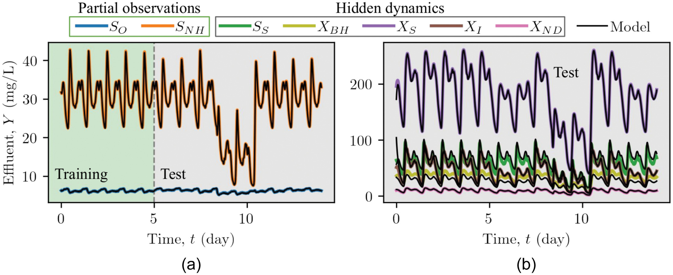
Motivated by the observed robust performance, PINN is further explored for the hidden dynamics inferences based on partial observations. In Fig. 5, PINN is trained with data of all state variables for

t < 5 days

. In Fig. 6, PINN is only provided with data of

S_{O}

and

S_{N H}

for the training period. Fig. 6(a) shows, despite limited observations, PINN can still robustly predict the dynamics of

S_{O}

and

S_{N H}

with

R^{2} > 0.99

. A comparison between Figs. 5 and 6 demonstrates the prediction of

S_{O}

and

S_{N H}

by PINN (trained with partial observations) is an improvement over the common ML models (trained with all state variables). Moreover, Fig. 6(b) shows PINN can also infer the (hidden) dynamics of the state variables (

S_{S}

,

X_{NH}

,

X_{S}

,

X_{I}

,

X_{N D}

) that are not observed, with reasonable accuracy (

R^{2} = 0.82

, averaged over these state variables), although some deviations are observed for

S_{S}

and

X_{BH}

. PINN inference of the hidden dynamics results from all the state variables not being independent but are correlated and coupled through the underlying biological reaction processes. As this domain knowledge is formulated as an unsupervised learning component

L^{ASM} (θ, P)

, the observation/labels for the (hidden) state variables are not needed in the PINN training. In contrast, common ML models require observation/labels in their supervised training, as illustrated in Fig. 1, and hence are not suitable for hidden dynamics inference.

Fig. 6. Learning hidden dynamics from partial observation with PINN model for activated sludge reactor under wet weather loading conditions. $S_{O}$ , $S_{N H}$ , $S_{S}$ , $X_{B H}$ , $X_{S}$ , $X_{I}$ , and $X_{N D}$ are oxygen, ${NH}_{4}^{+} + {NH}_{3}$ nitrogen, readily biodegradable substrate, active heterotrophic biomass, slowly biodegradable substrate, particulate inert organic matter, particulate biodegradable organic nitrogen, respectively. $S_{O}$ and $S_{N H}$ are provided for PINNs training for $t < 5 days$ . $S_{S}$ , $X_{BH}$ , $X_{S}$ , $X_{I}$ , and $X_{N D}$ are the hidden state variables. The activated sludge reactor dynamics is defined in Eqs. (7) and (S2)–(S13).

Case 3. Fixed-Bed Granular Adsorption Reactor

Fig. 7 illustrates the time-space solution domains of the phosphorus dissolved phase

Y (t, x)

and adsorbed phase

q (t, x)

of fixed-bed granular adsorption reactor in PINNs as 2D contours. The vertical axis of the contour is the spatial coordinate

x

and illustrates the spatial distribution of the TDP along the reactor length (normalized by total granular bed length,

L_{b}

). The horizontal axis of the contour is time

t

and illustrates the evolution of the TDP profile in time. The left boundary of the 2D contour represents the initial conditions (

t = 0

). The bottom and top boundaries are the influent boundary (

x = 0

, where TDP is loading the reactor) and the effluent boundary (

x = L_{b}

, the location of TDP breakthrough). The orange cross markers illustrate the solutions where the clean bed condition

Y (0, x)

is imposed. The green cross markers show the solutions where the reactor influent loading is defined; in this case,

Y (t, 0) = 0.5 mg / L

. The red cross markers are where the effluent TDP is measured from the physical modeling (i.e., data from adsorption experiments). These orange, green, and red markers are where the supervised learning takes place through the loss functions of

L^{IC} (θ)

,

L^{BC} (θ)

, and

L^{data} (θ)

in PINNs.

Fig. 7. Prediction of PINNs in fixed-bed granular adsorption reactor. Plots (a) and (b) are the time-space solution surfaces for the dissolved phase and adsorbed phase TDP. $Y$ is the TDP concentration. $Y^{I}$ is the influent TDP concentration. $q$ is the mass fraction of the adsorbed phase and adsorbent (kg adsorbed/kg adsorbent). IC and BC are initial conditions and boundary conditions. The fixed-bed granular adsorption reactor dynamics is defined in Eqs. (8)–(10). The physical model results are from Sansalone and Ma (2011).

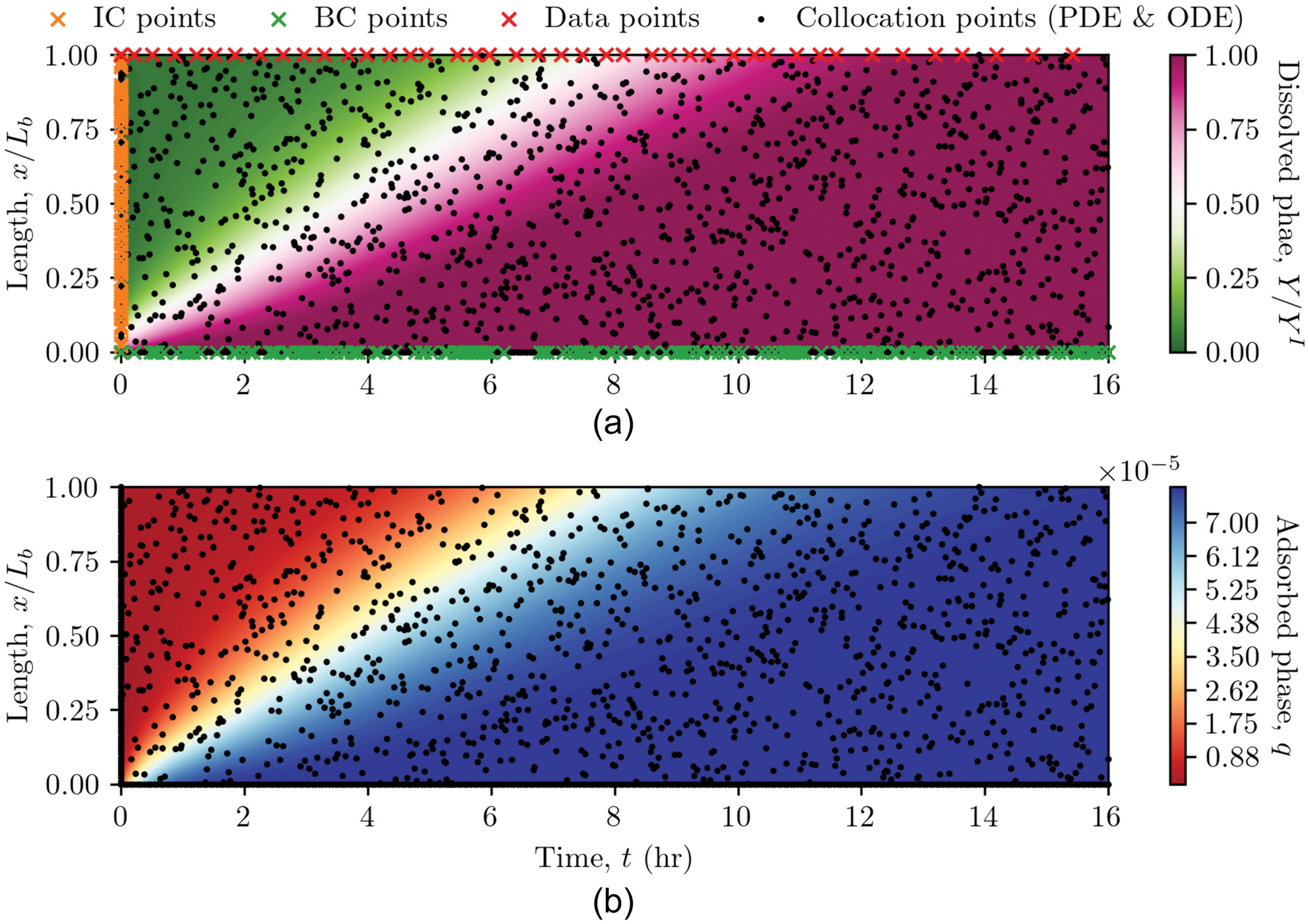
As illustrated by Fig. 7(a), these supervised learning points constitute a small fraction of the solution domain (located on the plot edges as initial and boundary conditions as well as data points collected of breakthrough from the physical modeling). If a common ANN model is implemented and trained with only these data points, the common ANN model will not infer the reactor dynamics and fails to generalize. This is because there can be an infinite number of surfaces (with different solutions) that perfectly fit the points on these edges; however, a common ANN model cannot differentiate which solution surface corresponds to the physical solution. An example is shown in Fig. S6 in the online supplemental materials. PINNs overcome this issue by configuring additional collocation points across the solution space, as represented by the black dot markers in Fig. 7(b). At these collocation points, the unsupervised learning based on the physics principles [as illustrated in Fig. 2(d)] is performed to guide the ML training and ensure the resulting solution surface is the physical solution.

Through the training, PINN learned the solution that simultaneously satisfies the physics and matches the physical modeling effluent results. As illustrated in Fig. 7(a), the reactor granular bed is initially clean, without any adsorption of TDP. After the reactor is loaded by the TDP solution, the TDP is adsorbed by the high surface area adsorbent, and the adsorbed phase TDP increases, as shown in Figs. 7(b). As time elapses, the TDP mass transfer zone penetrates through the reactor granular bed with eventual breakthrough of TDP in the reactor effluent. The PINNs model prediction of the TDP breakthrough curve

Y (t, L_{b})

agrees well with physical adsorption modeling results, as shown in Fig. 8(d). Note there are no data of the adsorbed phase

q

provided for PINN training, the solution and hidden dynamics of adsorbed phase

q (t, x)

is completely inferred by PINNs through the underlying physics.

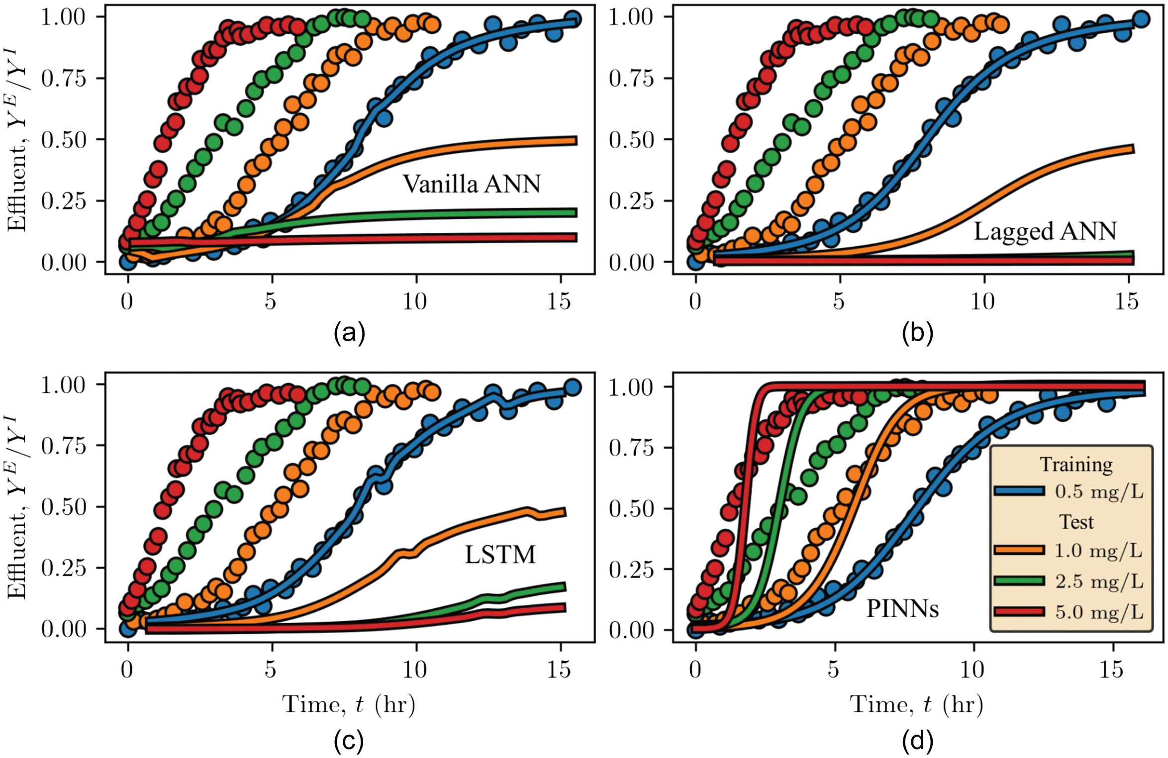
Fig. 8. Prediction of common ML and PINN models for fixed-bed granular adsorption reactor subject to different loadings. $Y^{I}$ and $Y^{E}$ are the influent and effluent TDP concentrations. A loading condition of $0.5 mg / L$ is used for training. Loading conditions of 1.0, 2.5, and $5.0 mg / L$ are used for testing model generalizability. The fixed-bed granular adsorption reactor dynamics are defined in Eqs. (8)–(10). Coefficients of determination ( $R^{2}$ ) are summarized in Table S7 in the online supplemental material. The physical model results are from Sansalone and Ma (2011).

Further, through the training, PINNs not only learns the ANN model parameter

θ

but also the forward adsorption constant

k_{f}

and hydrodynamic dispersion coefficient tensor

D_{h}

from the reactor dynamics. With these learned physical parameters

(k_{f}, D_{h})

, PINN is applied to predict the reactor dynamics for different TDP loading of 1.0, 2.5, and

5.0 mg / L

(i.e., out of sample data sets). Fig. 8 examines and compares the generalizability of common ML and PINNs when these models are applied to loading conditions that the model have not “seen” during the training. Table S7 in the online supplemental material summarizes the coefficient of determination (

R^{2}

) of these models, as defined in Eq. (S1). Fig. 8 and Table S7 show that PINNs generalize and predict the reactor response as influent TDP load increases. As the influent TDP load increases, the mass transfer zone progresses at a higher rate toward the axial reactor outlet, and the TDP breakthrough occurs as the adsorptive media capacity is exhausted more rapidly. PINN predictions yield

R^{2}

of 0.75 (averaged over test cases of 1.0, 2.5, and

5.0 mg / L

) with respect to the physical modeling results. Whereas common ML models, while yielding good performance during the training (indicated by good agreements with

Y^{I} = 0.5 mg / L

), fail to generalize for these “unseen” loading conditions. Common ML models predict a nonphysical reactor response; the reactor is exhausted slower as the influent TDP increases.

Discussion

Limitations and Benefits of Common Machine Learning for Water System UOP Modeling

Common machine learning (ML) models generate predictions by learning the patterns of the data in contrast with learning the underlying mechanics embedded in the data (Lai et al. 2017). Extracting patterns from data and leveraging these patterns for predictions can be an effective solution for many engineering and scientific applications, as demonstrated by the literature in computer vision (CV) and natural language processing (NPL) (Spencer et al. 2019). The recent success of ChatGPT and GPT 4 are prime examples (OpenAI 2023). For urban water system UOPs, patterns of the system dynamics can also be beneficial for system modeling. As shown by the CSTR case in Fig. 3(a) and activated sludge reactor case in Fig. 5(c), when the system dynamics exhibit periodic patterns, common ML models can exploit these features and predict the system dynamics. This observation is also supported by recent literature (Zhi et al. 2021), in which LSTM can predict the periodic seasonal variation of dissolved oxygen in rivers in the United States.

However, relying on data patterns for dynamics prediction may not be a sufficient and robust solution for water systems subject to more complex unsteady loadings and dynamics, as is the case for many urban water UOPs. As illustrated by Case 1 in Fig. 3, common ML models largely deviate from the CSTR solution as soon as the model is extended beyond the training period. The CSTR examined in this study is arguably one of the simplest reactor configurations in urban water treatment systems. Yet, common ML models fail to predict CSTR behavior. Most urban water treatment systems are subject to more complex physical operations and also chemical and biological processes involving turbulent mixing, multiphase interactions, exothermic reactions, etc. The application of common ML models to these systems and conditions can be challenging. Future research is needed to investigate the predictive capability of common ML models for urban water treatment systems with levels of complexity, as shown herein. Common examples include stormwater treatment systems such as engineered ponds and green infrastructure. In particular, the predictive capability of common ML models, whether such models are predictive or not, should be documented and elucidated in future research. ML model forensics, even in cases where such models are not predictive, can offer valuable insights as on the basis of “lessons learned” and provide future guidance.

In contrast with the conformal thinking that “data are the limiting factor for ML,” this study illustrates that limitations of common ML models for prediction water system dynamics can be more associated with the fundamental model formulations of supervised learning (i.e., regression) rather than the sampling frequency of training data, detailed ML model structure, and the model training process. Fig. 9 illustrates that providing more sampling frequency, changing model structure, and altering the learning rate only improves the performance of common ML models to a limited extent. These observations imply that while sufficient data are essential, the quantity of data may not be the limiting factor in the application of common ML models for water system UOP modeling. When the water system dynamics are subject to a higher dimension, simply feeding more data to train common ML models may not overcome the fundamental limitation imposed by the “black box” formulation (i.e., agnostic to physics) for generalization and extrapolation. A common example is the use of residence time (RT) to infer stormwater clarifier “pond” performance which considers the pond as a “black-box” irrespective of hydrodynamics, partitioning, particle size distributions and specific gravity and internal/external geometrics. A significant amount of the recent literature on ML application in water systems has emphasized the importance of collecting more data for ML model training (Huang et al. 2021; Li et al. 2021a). This can be true from a statistical learning perspective. Given sufficient and diverse data, ultimately ML makes predictions, as interpolation and reasonable performance should be expected. In the case of urban water system modeling, more often than not, high sampling cost prevents obtaining more data for ML model training. This study further extends the previous research and demonstrates that, under the economic constraints of data sampling, more sampling may benefit ML model training but may not practically overcome the fundamental limitation of common ML models in generalization and extrapolation.

Fig. 9. LSTM model prediction for a CSTR with various (a) model structures; and (b) training data size. The CSTR configuration and loading conditions are identical to those in Fig. 3(d). $N_{d}$ is training data size, $N_{h}$ is the number of features in the hidden state, and $N_{l}$ is the number of the recurrent layers.

Notwithstanding these limitations, common ML models demonstrate high flexibility and are readily implementable; these are important model attributes. The same ML models illustrated in Fig. 1 can be applied to predict different system dynamics with minimal adaption. In fact, only the input and output layers need to be modified according to a specific application, thus recognizing the model hyperparameters that may need to be retuned for optimal model performance. Such high flexibility and adaptability allow these ML models to be efficiently applied for a wide range of engineering and science applications. In addition, common ML models may also be advantageous in applications that lack domain knowledge or where domain knowledge is challenging to apply. One such example is the modeling of complex hydrologic processes (Beven 2020), in which an accurate delineation and definition of control volume/boundaries for applying mass conservation (i.e., water mass/volume balance) is challenging. For such applications, a data-driven solution with common ML models may outperform a deficient process description based on the system’s domain knowledge. However, in purely data-driven applications such as time series forecasting of stocks, tourism, transportation, demographics (i.e., Makridakis competitions), researchers also observed that pure ML models might not be as robust as classic statistical methods [e.g., autoregressive moving average (ARMA) or autoregressive integrated moving average (ARIMA)] (Makridakis et al. 2020; Gilliland 2020).

Potential and Challenges of Scientific Machine Learning (SciML) for Water System UOP Modeling

PINNs illustrated herein, while new, share many philosophical similarities with data fusion and data assimilation, i.e., combining theory with observations for better prediction performance. PINNs (and by extension SciML) incorporate domain knowledge into the ML framework through novel ML architecture, as illustrated in Fig. 2. By imposing the domain knowledge as an unsupervised learning component in the ML loss function, the solution space is constrained/regularized, and the ML model is guided to learn the underlying system dynamics that generate the observed data, as opposed to only learning the pattern in the data (e.g., common ML models). As illustrated by the diverse cases examined in Figs. 3, 5, and 8, PINNs yield significantly improved predictive capability and generalizability compared with common ML models, whether for time-varying or time-space dependent water system dynamics.

Compared with common ML models, PINNs require much less data for model training and are less prone to overfitting. This is one of the benefits of imposing domain knowledge to regulate the model solution. As illustrated in Fig. S6 in the online supplemental materials, four data points are sufficient for PINNs to learn and predict the dynamics of the CSTR system. In contrast, common ML models are challenging to develop with these limited data. This attribute of PINNs is particularly important and beneficial for urban water system modeling, where data are often sparse due to sampling/analytical challenges and economic resources. One such example is the monitoring and modeling of stormwater treatment systems. Field monitoring of stormwater systems has a high cost, ranging from 250,000 to 700,000 USD as of 2015 (National Stormwater Testing and Evaluation of Products and Practices Workgroup 2014; Chesapeake Bay Scientific and Technical Advisory Committee 2015; Li and Sansalone 2020). Yet, higher-frequency sampling remains economically unfeasible since influent/effluent samples require laboratory analysis as part of most regulatory certifications, which is a major cost component of monitoring campaigns. Direct assessment of the system dynamics with sparse samples can result in aliasing errors and mislead the interpretation of system performance. In such a scenario, PINNs can be effectively applied to reconstruct, recover, and inform the system dynamics based on sparse data, as illustrated in Fig. S6. Similarly, PINNs can also infer system dynamics with sparse data in space. As demonstrated by the fixed-bed granular adsorption reactor case in Figs. 7 and 8, PINNs can infer the entire 2D solution domain with only sparse sampling at the top boundary (i.e., effluent data).

Another benefit provided by the novel architecture of PINNs is the capability for simultaneous parameter estimation (Raissi et al. 2019; Yazdani et al. 2020). As illustrated by the three UOP cases, PINNs can inversely identify the model parameter

P

embedded in the data. As these model parameters

P

each have a physical basis, once learned, these parameters allow PINNs to extrapolate and generalize to a future time (i.e., forecast as illustrated in the three cases) and to loading conditions that are distinct from the training data (Fig. 8). Additionally, incorporating unsupervised learning based on domain knowledge provides PINNs with the capability for hidden dynamics inference (i.e., no label is needed for training). As illustrated by the activated sludge reactor case and fixed-bed granular adsorption reactor case, PINNs can infer the state variables in a UOP, i.e., variables that were not directly observed. In water system modeling, this feature of PINNs can potentially overcome several challenges and limitations with real-time monitoring and control of water systems. For example, in wastewater treatment, several critical variables such as heterotrophic biomass

X_{BH}

, readily biodegradable soluble substrate

S_{S}

, and slowly biodegradable substrate

X_{S}

cannot be directly measured online (Hedegärd and Wik 2011). As demonstrated by the activated sludge reactor case in Fig. 6, PINNs can infer the real-time dynamics of these variables based on the variables (e.g., dissolved oxygen

S_{O}

and

{NH}_{4}^{+} + {NH}_{3}

nitrogen

S_{N H}

) that can be measured with online sensors. Note that these aforementioned tasks of parameter estimation and hidden dynamics inference are classified as inverse problems. Conventional mechanistic models are not immediately applicable and require coupling with optimization algorithms. Inverse problems, especially when constituted by a PDE, can greatly challenge the mechanistic models due to the high computational cost associated with exploring large parameter space. In contrast, PINNs simultaneously explore the parameter space and learn the mapping in each backpropagation iteration during the training, yielding increased computational efficiency.

This study has demonstrated the potential and benefits of PINNs for urban water system modeling, especially when compared with common ML models. However, as an emerging and maturing field, there are also challenges associated with applying PINNs to water system modeling. In the presence of unseen or varied system loading conditions (e.g., hydrograph changes or variations in loading concentration), the success of PINNs often hinges on a robust understanding of the system’s dynamics. For systems whose dynamics can be effectively described by differential equations, PINNs offer enhanced generalizability in comparison with common ML models. In such cases, the generalizability of PINNs to unseen or varied system loading conditions becomes less of a concern. This is because the underlying differential equation model directly supports PINNs’ generalization abilities, effectively treating changes in loading conditions as equivalent to alterations in the boundary conditions of the differential equations, as exemplified in Case 3. At the same time, unlike common ML models, PINN model architecture is problem-specific, and a one-size-fits-all model does not exist. Users need to formulate and incorporate the domain knowledge into PINNs based on the intended application. This can be a challenge for PINNs in civil and environmental engineering applications, in cases where scientific computing has not yet been integrated into the curricula, as recently identified by the American Society of Civil Engineers (Liu and Zhang 2019; Liu et al. 2020; Li and Sansalone 2022b). Nevertheless, several open-source and commercial packages have been developed to simplify and streamline the PINN model development, such as DeepXDE (Lu et al. 2021), NeuralPDE (Zubov et al. 2021), and Nvidia Modulus. Another difficulty of PINNs is associated with model training for parameters of larger and more complex models. As illustrated by Krishnapriyan et al. (2021), a constraint imposed by the domain knowledge in the PINN loss function is significantly different from common regulation techniques that are based on the

L 1

and

L 2

norm (e.g., ridge regularizer, lasso regularizer, elastic net regularizer) (Géron 2019). The inclusion of this constraint

L (P)

can significantly complicate the loss function landscape and pose challenges for the model training. In this study, these difficulties are overcome through the curriculum training strategies: the model is first trained with an easier problem (i.e., smaller model parameter) and the problem complexity is gradually increased, as suggested by Krishnapriyan et al. (2021). Yet, future research is needed to investigate and improve the robustness and efficiency of PINN training. Developing a more robust and automated training method can be critical to adopting and applying PINNs in research and translating this to engineering practice. In addition, future efforts should be considered for developing a well-documented and public database of various urban water systems to further benchmark and examine ML models and PINNs under more complex system dynamics.

Conclusions

This study examines the predictive capability and generalizability of ML models in comparison with SciML as PINN models for urban water system modeling. Common ML models for water system modeling are synthesized based on the literature and represented by vanilla ANN, lagged ANN, and LSTM. PINN models are developed for UOP examples that are commonly encountered in water, wastewater, and stormwater treatment: (1) CSTR; (2) activated sludge reactor; and (3) fixed-bed granular adsorption reactor. From the scope of this study, the results yield the following conclusions:

•

Common ML methods for water system modeling, while diverse in the details of the model implemented, are largely similar in the formulation of supervised machine learning (ML). Common ML methods based on a neural network can be synthesized and classified into three categories: (1) instant mapping method; (2) time-lagged mapping method (also known as sliding window); and (3) RNN such as LSTM. The data layout, training formulation, and model structure are summarized in the section “Common machine learning models” and Fig. 1. These summaries and generalizations can facilitate efficient application and adaption of common ML methods for a wide range of urban water systems and UOP modeling. Future research, while benefiting from the possibilities and opportunities that common ML models enable and provide, should examine the robustness of common ML models; as common ML models are “black box” and agnostic to physics.

•

When the data are limited, common ML methods represented by vanilla ANN, lagged ANN, and LSTM are not robust for water system UOP modeling for the cases of common UOPs and conditions examined. As illustrated in Figs. 3 and 5, except for system dynamics that exhibit simpler periodic patterns, predictions from common ML models substantially deviate from the solutions for systems subject to more complex loadings. Even for a simple CSTR case, the performance of common ML models degrades as soon as the model is extended beyond the training period. Further investigation illustrates that increasing training data and optimizing model hyperparameters do not overcome these limitations of common ML models. These limitations in common ML models are potentially associated with the fundamental formulation of supervised ML for water system modeling as a “black box” (i.e., agnostic to physics). These limitations can be overcome by integrating domain knowledge into ML models through novel ML model architectures such as SciML.

•

As a type of SciML, PINNs demonstrate improved predictive capability and generalizability for urban water system UOP modeling as compared with common ML models. Imposing domain knowledge as constraints in the loss function can guide PINNs to learn the underlying system dynamics embedded in the data. For the three distinct, yet common, UOP cases examined, PINNs robustly predict the system dynamics, whether for time-varying or time-space variability. PINNs can also generalize to loading conditions distinct from the training data. In addition, embedding domain knowledge into the model architecture provides PINNs with the capability to infer and reconstruct hidden system dynamics with sparse time-spatial data or even partial observations. These results demonstrate the significant potential of PINNs for hybrid data-driven physics-informed water system UOP modeling and illustrate the possibility of PINNs to address problems (e.g., parameter estimation and hidden dynamics inference) that are challenging for ML or scientific computing. Such a confluence of ML and domain knowledge in SciML represents a promising approach and solution toward robust modeling of urban water systems that are subject to episodic or complex time-space variability.

Notation

The following symbols are used in this paper:

$b_{H}$: decay coefficient for heterotrophic biomass;
$D_{h}$: hydrodynamic dispersion coefficient tensor;
$f (\cdot)$: governing function;
$I$: identity matrix;
$i$: index of data pairs;
$K$: adsorption equilibrium constant;
$K_{s}$: half-saturation coefficient for $X_{BH}$ ;
$K_{L}$: oxygen transfer coefficient;
$K_{O H}$: oxygen half-saturation coefficient for $X_{BH}$ ;
$K_{X}$: half-saturation coefficient for hydrolysis of $X_{S}$ ;
$k$: first-order reaction constant;
$\hat{k}$: inferred first-order reaction constant;
$k_{a}$: ammonification coefficient;
$k_{f}$: forward (adsorption) constant;
$k_{h}$: maximum specific hydrolysis rate;
$k_{r}$: reverse (desorption) constant;
$L$: loss function;
$L^{ASM}$: loss function for ASM model;
$L^{BC}$: loss function of boundary condition;
$L^{CSTR}$: loss function for CSTR model;
$L^{IC}$: loss function of initial condition;
$L^{ODE}$: loss function for ODE;
$L^{PDE}$: loss function for PDE;
$L^{data}$: data loss function;
$L^{f}$: loss function of governing function;
$m$: number of outputs;
$N$: number of paired data sets;
$N_{BC}$: number of data pairs for boundary conditions;
$N_{IC}$: number of data pairs for initial conditions;
$N_{d}$: total number of data pairs;
$N_{f}$: number of collocations points;
$N_{h}$: number of features in the hidden state;
$N_{l}$: number of recurrent layers;
$n$: number of inputs;
$P$: model parameter in governing functions;
$Q^{E}$: outflow;
$Q^{I}$: inflow;
$q$: mass fraction of the adsorbed phase;
$q_{\max}$: adsorption capacity;
$R$: reaction rate vector;
$R$: total/net reaction rate;
$R^{2}$: coefficient of determination;
$R^{r \times s}$: $r$ by $s$ matrix with real numbers;
$S_{ALK}$: alkalinity;
$S_{I}$: soluble inert organic matter;
$S_{N D}$: soluble biodegradable organic nitrogen;
$S_{N H}$: ${NH}_{4}^{+} + {NH}_{3}$ nitrogen;
$S_{N O}$: nitrate and nitrite nitrogen;
$S_{O}$: oxygen;
$S_{O}^{*}$: oxygen saturation concentration;
$S_{S}$: readily biodegradable substrate;
$t$: time;
$u$: superficial velocity vector;
$u$: X-component pore velocity;
$u_{p}$: pore velocity vector;
$u_{p}$: X-component superficial velocity;
$V$: system volume;
$v$: Y-component pore velocity;
$v_{p}$: Y-component superficial velocity;
$w$: Z-component pore velocity;
$w_{p}$: Z-component superficial velocity;
$X$: input tensor;
$X_{c}^{(t)}$: inputs matrix for $t$ data pair;
$x^{(t)}$: inputs vector for $t$ data pair;
$x_{v}^{(t)}$: reshaped inputs vector for $t$ data pair;
$X_{BA}$: active autotrophic biomass;
$X_{BH}$: active heterotrophic biomass;
$X_{I}$: particulate inert organic matter;
$X_{N D}$: particulate biodegradable organic nitrogen;
$X_{P}$: particulate products arising from biomass decay;
$X_{S}$: slowly biodegradable substrate;
$x$: X-coordinate;
$Y$: state variables;
$Y^{I}$: influent species concentration vector;
$Y^{E}$: effluent species concentration vector;
$y$: output tensor;
$y^{(t)}$: outputs vector for $t$ data pair;
$y^{(t + 1)}$: outputs vector for $t + 1$ data pair;
$Y$: species concentration;
$Y^{I}$: influent species concentration;
$Y^{E}$: effluent species concentration;
$y$: Y-coordinate;
$z$: Z-coordinate;
$β$: specific mass divided by porosity;
$\hat{η}$: unit vector for dissolved oxygen;
$θ$: model parameters;
$λ^{BC}$: weighting factor for boundary conditions loss;
$λ^{IC}$: weighting factor for initial conditions loss;
$λ^{f}$: weighting factor for function loss;
$μ_{H}$: maximum specific growth rate for $X_{B H}$ ;
$ρ_{p}$: granular media density;
$τ$: lagged time period;
$ϕ$: reactor porosity; and
$X$: space coordinate vector.

Supplemental Materials

File (supplemental_materials_joeedu.eeeng-7467_li.pdf)

Download
3.11 MB

Data Availability Statement

All data, models, or code that support the findings of this study are available from the corresponding author upon reasonable request.

Acknowledgments

This research was supported by the United States Geological Survey (USGS) 104B Program through the Tennessee Water Resources Research Center (TNWRRC) at University of Tennessee, Knoxville, through the Water Resources Research Institute at the University of Florida, and by the University of Florida Informatics Institute (UFII) SEED Funds. This research was also supported by the project Modeling Water Management System Clarification at APF (Project #AGR00029097) through EG Solutions, Inc. from Naples Airport Authority. The author would like to acknowledge the contribution of Dr. Jia Ma for conducting the physical experiments.

References

Abdalla, E. M. H., V. Pons, V. Stovin, S. De-Ville, E. Fassman-Beck, K. Alfredsen, and T. M. Muthanna. 2021. “Evaluating different machine learning methods to simulate runoff from extensive green roofs.” Hydrol. Earth Syst. Sci. 25 (11): 5917–5935. https://doi.org/10.5194/hess-25-5917-2021.

Google Scholar

Abdeldayem, O. M., A. M. Dabbish, M. M. Habashy, M. K. Mostafa, M. Elhefnawy, L. Amin, E. G. Al-Sakkari, A. Ragab, and E. R. Rene. 2022. “Viral outbreaks detection and surveillance using wastewater-based epidemiology, viral air sampling, and machine learning techniques: A comprehensive review and outlook.” Sci. Total Environ. 803 (Jan): 149834. https://doi.org/10.1016/j.scitotenv.2021.149834.

Google Scholar

Adeel, Z., and R. G. Luthy. 1995. “Sorption and transport kinetics of a nonionic surfactant through an aquifer sediment.” Environ. Sci. Technol. 29 (4): 1032–1042. https://doi.org/10.1021/es00004a025.

Google Scholar

Alex, J., L. Benedetti, J. Copp, K. Gernaey, U. Jeppsson, I. Nopens, M. Pons, J. Steyer, and P. Vanrolleghem. 2018. Benchmark simulation model no. 1 (BSM1). London: International Water Association.

Google Scholar

Antanasijević, D., V. Pocajt, D. Povrenović, A. Perić-Grujić, and M. Ristić. 2013. “Modelling of dissolved oxygen content using artificial neural networks: Danube River, North Serbia, case study.” Environ. Sci. Pollut. Res. 20 (Dec): 9006–9013. https://doi.org/10.1007/s11356-013-1876-6.

Google Scholar

Bear, J. 1972. Dynamics of fluids in porous media. New York: Dover.

Google Scholar

Beven, K. 2020. “Deep learning, hydrological processes and the uniqueness of place.” Hydrol. Processes 34 (16): 3608–3613. https://doi.org/10.1002/hyp.13805.

Google Scholar

Brockwell, P. J., and R. A. Davis. 2016. Introduction to time series and forecasting. Springer texts in statistics. Berlin: Springer. https://doi.org/10.1007/978-3-319-29854-2.

Google Scholar

Brunton, S. L., and J. N. Kutz. 2019. Data-driven science and engineering: Machine learning, dynamical systems, and control. Cambridge, UK: Cambridge University Press. https://doi.org/10.1017/9781108380690.

Google Scholar

Chen, R. T. Q., Y. Rubanova, J. Bettencourt, and D. Duvenaud. 2018. “Neural ordinary differential equations.” In Proc., Advances in Neural Information Processing Systems 31 (NeurIPS), 31–60. Ithaca, NY: Cornell Univ.

Google Scholar

Chesapeake Bay Scientific and Technical Advisory Committee, 2015. Evaluating proprietary BMPs: Is it time for a state, regional or national program? Fairfax, VA: Chesapeake Bay Scientific and Technical Advisory Committee.

Google Scholar

Deng, Y. 2020. “Low-cost adsorbents for urban stormwater pollution control.” Front. Environ. Sci. Eng. 14 (5): 1–8. https://doi.org/10.1007/s11783-020-1262-9.

Google Scholar

French, M. N., W. F. Krajewski, and R. R. Cuykendall. 1992. “Rainfall forecasting in space and time using a neural network.” J. Hydrol. 137 (1–4): 1–31. https://doi.org/10.1016/0022-1694(92)90046-X.

Google Scholar

Géron, A. 2019. Hands-on machine learning with Scikit-Learn and TensorFlow. Newton, MA: O’Reilly Media.

Google Scholar

Ghattas, O., and K. Willcox. 2021. “Learning physics-based models from data: Perspectives from inverse problems and model reduction.” Acta Numer. 30 (May): 445–554. https://doi.org/10.1017/S0962492921000064.

Google Scholar

Gilliland, M. 2020. “The value added by machine learning approaches in forecasting.” Int. J. Forecasting 36 (1): 161–166. https://doi.org/10.1016/j.ijforecast.2019.04.016.

Google Scholar

Godo-Pla, L., P. Emiliano, F. Valero, M. Poch, G. Sin, and H. Monclús. 2019. “Predicting the oxidant demand in full-scale drinking water treatment using an artificial neural network: Uncertainty and sensitivity analysis.” Process Saf. Environ. Prot. 125 (May): 317–327. https://doi.org/10.1016/j.psep.2019.03.017.

Google Scholar

Grady, C. P. L., G. T. Daigger, N. G. Love, and C. D. M. Filipe. 2011. Biological wastewater treatment. Boca Raton, FL: CRC Press.

Crossref

Google Scholar

Griffiths, K. A., and R. C. Andrews. 2011. “Application of artificial neural networks for filtration optimization.” J. Environ. Eng. 137 (11): 1040–1047. https://doi.org/10.1061/(ASCE)EE.1943-7870.0000439.

Google Scholar

Guo, H., K. Jeong, J. Lim, J. Jo, Y. M. Kim, J.-P. Park, J. H. Kim, and K. H. Cho. 2015. “Prediction of effluent concentration in a wastewater treatment plant using machine learning models.” J. Environ. Sci. 32 (Jun): 90–101. https://doi.org/10.1016/j.jes.2015.01.007.

Google Scholar

Hedegärd, M., and T. Wik. 2011. “An online method for estimation of degradable substrate and biomass in an aerated activated sludge process.” Water Res. 45 (19): 6308–6320. https://doi.org/10.1016/j.watres.2011.09.003.

Google Scholar

Henze, M., C. P. Grady, W. Gujer, G. V. Marais, and T. Matsuo. 1987. “A general model for single-sludge wastewater treatment systems.” Water Res. 21 (5): 505–515. https://doi.org/10.1016/0043-1354(87)90058-3.

Google Scholar

Hochreiter, S., and J. Schmidhuber. 1997. “Long short-term memory.” Neural Comput. 9 (8): 1735–1780. https://doi.org/10.1162/neco.1997.9.8.1735.

Google Scholar

Horgue, P., C. Soulaine, J. Franc, R. Guibert, and G. Debenest. 2015. “An open-source toolbox for multiphase flow in porous media.” Comput. Phys. Commun. 187 (Feb): 217–226. https://doi.org/10.1016/j.cpc.2014.10.005.

Google Scholar

Huang, R., C. Ma, J. Ma, X. Huangfu, and Q. He. 2021. “Machine learning in natural and engineered water systems.” Water Res. 205 (Oct): 117666. https://doi.org/10.1016/j.watres.2021.117666.

Google Scholar

Huber, W. C., L. Cannon, and M. Stouder. 2006. BMP modeling concepts and simulation. Washington, DC: USEPA.

Google Scholar

Istok, J. 1989. “Derivation of equations of solute transport.” In Groundwater modeling by the finite element method, 469–477. Washington, DC: American Geophysical Union.

Crossref

Google Scholar

IWA (International Water Association). 2023. “Modelling & integrated assessment.” Accessed January 9, 2023. https://iwa-mia.org/benchmarking/.

Google Scholar

Jia, Y., F. Zheng, H. R. Maier, A. Ostfeld, E. Creaco, D. Savic, J. Langeveld, and Z. Kapelan. 2021. “Water quality modeling in sewer networks: Review and future research directions.” Water Res. 202 (Sep): 117419. https://doi.org/10.1016/j.watres.2021.117419.

Google Scholar

Kaptanoglu, A. A., et al. 2022. “PySINDy: A comprehensive Python package for robust sparse system identification.” J. Open Source Software 7 (69): 3994. https://doi.org/10.21105/joss.03994.

Google Scholar

Karniadakis, G. E., I. G. Kevrekidis, L. Lu, P. Perdikaris, S. Wang, and L. Yang. 2021. “Physics-informed machine learning.” Nat. Rev. Phys. 3 (6): 422–440. https://doi.org/10.1038/s42254-021-00314-5.

Google Scholar

Krajewski, A., A. E. Sikorska, and K. Banasik. 2017. “Modeling suspended sediment concentration in the stormwater outflow from a small detention pond.” J. Environ. Eng. 143 (10): 05017005. https://doi.org/10.1061/(ASCE)EE.1943-7870.0001258.

Google Scholar

Krishnapriyan, A. S., A. Gholami, S. Zhe, R. M. Kirby, and M. W. Mahoney. 2021. “Characterizing possible failure modes in physics-informed neural networks.” Preprint, submitted September 2, 2021. https://arxiv.org/abs/2109.01050.

Google Scholar

Lai, G., W. C. Chang, Y. Yang, and H. Liu. 2017. “Modeling long- and short-term temporal patterns with deep neural networks.” In Proc., 41st Int. ACM SIGIR Conf. on Research and Development in Information Retrieval, SIGIR 2018, 95–104. New York: Association for Computing Machinery.

Google Scholar

Lara-Benítez, P., M. Carranza-García, and J. C. Riquelme. 2021. “An experimental review on deep learning architectures for time series forecasting.” Int. J. Neural Syst. 31 (3): 2130001. https://doi.org/10.1142/S0129065721300011.

Google Scholar

Lawrence Livermore National Laboratory. 2023. “ODEPACK | Computing.” Accessed March 14, 2023. https://computing.llnl.gov/projects/odepack.

Google Scholar

Li, F., and P. A. Vanrolleghem. 2022. “An influent generator for WRRF design and operation based on a recurrent neural network with multi-objective optimization using a genetic algorithm.” Water Sci. Technol. 85 (5): 1444–1453. https://doi.org/10.2166/WST.2022.048.

Google Scholar

Li, H., and J. Sansalone. 2020. “CFD as a complementary tool to benchmark physical testing of PM separation by unit operations.” J. Environ. Eng. 146 (11): 04020122. https://doi.org/10.1061/(ASCE)EE.1943-7870.0001803.

Google Scholar

Li, H., and J. Sansalone. 2022a. “A CFD-ML augmented alternative to residence time for clarification basin scaling and design.” Water Res. 209 (Feb): 117965. https://doi.org/10.1016/j.watres.2021.117965.

Google Scholar

Li, H., and J. Sansalone. 2022b. “Implementing machine learning to optimize the cost-benefit of urban water clarifier geometrics.” Water Res. 220 (Jul): 118685. https://doi.org/10.1016/j.watres.2022.118685.

Google Scholar

Li, H., and J. Sansalone. 2022c. “InterAdsFoam: An open-source CFD model for granular media–adsorption systems with dynamic reaction zones subject to uncontrolled urban water fluxes.” J. Environ. Eng. 148 (9): 04022049. https://doi.org/10.1061/(ASCE)EE.1943-7870.0002027.

Google Scholar

Li, K., H. Duan, L. Liu, R. Qiu, B. van den Akker, B. J. Ni, T. Chen, H. Yin, Z. Yuan, and L. Ye. 2022. “An integrated first principal and deep learning approach for modeling nitrous oxide emissions from wastewater treatment plants.” Environ. Sci. Technol. 56 (4): 2816–2826. https://doi.org/10.1021/acs.est.1c05020.

Google Scholar

Li, L., S. Rong, R. Wang, and S. Yu. 2021a. “Recent advances in artificial intelligence and machine learning for nonlinear relationship analysis and process control in drinking water treatment: A review.” Chem. Eng. J. 405 (Feb): 126673. https://doi.org/10.1016/j.cej.2020.126673.

Google Scholar

Li, S., A. E. Seyed, A. Emaminejad, S. Aguiar, A. Furneaux, X. Cai, and R. D. Cusick. 2021b. “Evaluating long-term treatment performance and cost of nutrient removal at water resource recovery facilities under stochastic influent characteristics using artificial neural networks as surrogates for plantwide modeling.” ACS ES&T Eng. 1 (11): 1517–1529. https://doi.org/10.1021/acsestengg.1c00179.

Google Scholar

Liu, D., J. J. Sansalone, and F. K. Cartledge. 2005. “Comparison of sorptive filter media for treatment of metals in runoff.” J. Environ. Eng. 131 (8): 1178–1186. https://doi.org/10.1061/(ASCE)0733-9372(2005)131:8(1178).

Google Scholar

Liu, K., K. Luo, Y. Cheng, A. Liu, H. Li, J. Fan, and S. Balachandar. 2023. “Surrogate modeling of parameterized multi-dimensional premixed combustion with physics-informed neural networks for rapid exploration of design space.” Combust. Flame 258 (Dec): 113094. https://doi.org/10.1016/j.combustflame.2023.113094.

Google Scholar

Liu, Q., D. Gui, L. Zhang, J. Niu, H. Dai, G. Wei, and B. X. Hu. 2022. “Simulation of regional groundwater levels in arid regions using interpretable machine learning models.” Sci. Total Environ. 831 (Jul): 154902. https://doi.org/10.1016/j.scitotenv.2022.154902.

Google Scholar

Liu, X., and J. Zhang. 2019. Computational fluid dynamics: Applications in water, wastewater, and stormwater treatment. Reston, VA: ASCE.

Google Scholar

Liu, X., J. Zhang, K. D. Nielsen, and Y. A. Cataño-Lopera. 2020. “Challenges and opportunities of computational fluid dynamics in water, wastewater, and stormwater treatment.” J. Environ. Eng. 146 (11): 02520002. https://doi.org/10.1061/(ASCE)EE.1943-7870.0001815.

Google Scholar

Lu, L., X. Meng, Z. Mao, and G. E. Karniadakis. 2021. “DeepXDE: A deep learning library for solving differential equations.” SIAM Rev. 63 (1): 208–228. https://doi.org/10.1137/19M1274067.

Google Scholar

Ly, Q. V., V. H. Truong, B. Ji, X. C. Nguyen, K. H. Cho, H. H. Ngo, and Z. Zhang. 2022. “Exploring potential machine learning application based on big data for prediction of wastewater quality from different full-scale wastewater treatment plants.” Sci. Total Environ. 832 (Aug): 154930. https://doi.org/10.1016/j.scitotenv.2022.154930.

Google Scholar

Makridakis, S., E. Spiliotis, and V. Assimakopoulos. 2020. “The M4 competition: 100,000 time series and 61 forecasting methods.” Int. J. Forecasting 36 (1): 54–74. https://doi.org/10.1016/j.ijforecast.2019.04.014.

Google Scholar

Mallat, S. 2016. “Understanding deep convolutional networks.” Philos. Trans. R. Soc. London, Ser. A 374 (2065): 20150203. https://doi.org/10.1098/RSTA.2015.0203.

Google Scholar

National Stormwater Testing and Evaluation of Products and Practices Workgroup. 2014. “Investigation into the feasibility of a national testing and evaluation program for stormwater products and practices.” Accessed May 20, 2020. https://www.wef.org/globalassets/assets-wef/2-resources/topics/o-z/stormwater/stormwater-institute/wef-stepp-white-paper_final_02-06-14.pdf.

Google Scholar

Newhart, K. B., J. E. Goldman-Torres, D. E. Freedman, K. B. Wisdom, A. S. Hering, and T. Y. Cath. 2020a. “Prediction of peracetic acid disinfection performance for secondary municipal wastewater treatment using artificial neural networks.” ACS ES&T Water 1 (2): 328–338. https://doi.org/10.1021/acsestwater.0c00095.

Google Scholar

Newhart, K. B., R. W. Holloway, A. S. Hering, and T. Y. Cath. 2019. “Data-driven performance analyses of wastewater treatment plants: A review.” Water Res. 157 (Jun): 498–513. https://doi.org/10.1016/j.watres.2019.03.030.

Google Scholar

Newhart, K. B., C. A. Marks, T. Rauch-Williams, T. Y. Cath, and A. S. Hering. 2020b. “Hybrid statistical-machine learning ammonia forecasting in continuous activated sludge treatment for improved process control.” J. Water Process Eng. 37 (Oct): 101389. https://doi.org/10.1016/j.jwpe.2020.101389.

Google Scholar

Ng, A. 2018. “Machine learning yearning.” Accessed February 16, 2020. https://www.deeplearning.ai/machine-learning-yearning/.

Google Scholar

OpenAI. 2023. “GPT-4 technical report.” Preprint, submitted March 15, 2023. https://arxiv.org/abs/2303.08774.

Google Scholar

Paszke, A., et al. 2019. “PyTorch: An imperative style, high-performance deep learning library.” In Proc., Advances in Neural Information Processing Systems 32. Cambridge, MA: The MIT Press.

Google Scholar

Pisa, I., I. Santin, A. Morell, J. L. Vicario, and R. Vilanova. 2019. “LSTM-based wastewater treatment plants operation strategies for effluent quality improvement.” IEEE Access 7 (Oct): 159773–159786. https://doi.org/10.1109/ACCESS.2019.2950852.

Google Scholar

Pyo, J. C., L. J. Park, Y. Pachepsky, S. S. Baek, K. Kim, and K. H. Cho. 2020. “Using convolutional neural network for predicting cyanobacteria concentrations in river water.” Water Res. 186 (Nov): 116349. https://doi.org/10.1016/j.watres.2020.116349.

Google Scholar

Quaghebeur, W., E. Torfs, B. De Baets, and I. Nopens. 2022. “Hybrid differential equations: Integrating mechanistic and data-driven techniques for modelling of water systems.” Water Res. 213 (Apr): 118166. https://doi.org/10.1016/j.watres.2022.118166.

Google Scholar

Rackauckas, C., Y. Ma, J. Martensen, C. Warner, K. Zubov, R. Supekar, D. Skinner, A. Ramadhan, and A. Edelman. 2020. “Universal differential equations for scientific machine learning.” Preprint, submitted January 13, 2020. https://arxiv.org/abs/2001.04385.

Google Scholar

Raissi, M., P. Perdikaris, and G. E. Karniadakis. 2019. “Physics-informed neural networks: A deep learning framework for solving forward and inverse problems involving nonlinear partial differential equations.” J. Comput. Phys. 378 (Feb): 686–707. https://doi.org/10.1016/j.jcp.2018.10.045.

Google Scholar

Recknagel, F., M. French, P. Harkonen, and K. I. Yabunaka. 1997. “Artificial neural network approach for modelling and prediction of algal blooms.” Ecol. Modell. 96 (1–3): 11–28. https://doi.org/10.1016/S0304-3800(96)00049-X.

Google Scholar

Sansalone, J., and J. Ma. 2011. “Parametric analysis and breakthrough modeling of phosphorus from Al-oxide filter media.” J. Environ. Eng. 137 (2): 108–118. https://doi.org/10.1061/(ASCE)EE.1943-7870.0000304.

Google Scholar

Sidhu, V., K. Barrett, D. Y. Park, Y. Deng, R. Datta, and D. Sarkar. 2021. “Wood mulch coated with iron-based water treatment residuals for the abatement of metals and phosphorus in simulated stormwater runoff.” Environ. Technol. Innovation 21 (Feb): 101214. https://doi.org/10.1016/j.eti.2020.101214.

Google Scholar

Spencer, B. F., V. Hoskere, and Y. Narazaki. 2019. “Advances in computer vision-based civil infrastructure inspection and monitoring.” Engineering 5 (2): 199–222. https://doi.org/10.1016/j.eng.2018.11.030.

Google Scholar

Sundui, B., O. A. Ramirez Calderon, O. M. Abdeldayem, J. Lázaro-Gil, E. R. Rene, and U. Sambuu. 2021. “Applications of machine learning algorithms for biological wastewater treatment: Updates and perspectives.” Clean Technol. Environ. Policy 23 (1): 127–143. https://doi.org/10.1007/s10098-020-01993-x.

Google Scholar

Taoufik, N., W. Boumya, M. Achak, H. Chennouk, R. Dewil, and N. Barka. 2022. “The state of art on the prediction of efficiency and modeling of the processes of pollutants removal based on machine learning.” Sci. Total Environ. 807 (Feb): 150554. https://doi.org/10.1016/j.scitotenv.2021.150554.

Google Scholar

Thompson, K. A., and E. R. Dickenson. 2021. “Using machine learning classification to detect simulated increases of de facto reuse and urban stormwater surges in surface water.” Water Res. 204 (Oct): 117556. https://doi.org/10.1016/j.watres.2021.117556.

Google Scholar

Trueman, B. F., W. James, T. Shu, E. Doré, and G. A. Gagnon. 2022. “Comparing corrosion control treatments for drinking water using a robust Bayesian generalized additive model.” ACS ES&T Eng. 3 (1): 15–25. https://doi.org/10.1021/acsestengg.2c00194.

Google Scholar

Valencia, A., W. Zhang, and N. B. Chang. 2021. “Integration of machine learning classifiers and higher order tensors for screening the optimal recipe of filter media in stormwater treatment.” Sci. Total Environ. 771 (Jun): 145423. https://doi.org/10.1016/j.scitotenv.2021.145423.

Google Scholar

Viet, N. D., and A. Jang. 2023. “Machine learning-based real-time prediction of micropollutant behaviour in forward osmosis membrane (waste) water treatment.” J. Cleaner Prod. 389 (Feb): 136023. https://doi.org/10.1016/j.jclepro.2023.136023.

Google Scholar

Wang, D., S. Thunéll, U. Lindberg, L. Jiang, J. Trygg, M. Tysklind, and N. Souihi. 2021. “A machine learning framework to improve effluent quality control in wastewater treatment plants.” Sci. Total Environ. 784 (Aug): 147138. https://doi.org/10.1016/j.scitotenv.2021.147138.

Google Scholar

Wu, G. D., and S. L. Lo. 2008. “Predicting real-time coagulant dosage in water treatment by artificial neural networks and adaptive network-based fuzzy inference system.” Eng. Appl. Artif. Intell. 21 (8): 1189–1195. https://doi.org/10.1016/j.engappai.2008.03.015.

Google Scholar

Yazdani, A., L. Lu, M. Raissi, and G. E. Karniadakis. 2020. “Systems biology informed deep learning for inferring parameters and hidden dynamics.” PLoS Comput. Biol. 16 (11): e1007575. https://doi.org/10.1371/journal.pcbi.1007575.

Google Scholar

Yu, J., N. Tang, and P. K. H. Lee. 2023. “Universal dynamics of microbial communities in full-scale textile wastewater treatment plants and system prediction by machine learning.” Environ. Sci. Technol. 57 (8): 3345–3356. https://doi.org/10.1021/acs.est.2c08116.

Google Scholar

Zaghloul, M. S., O. T. Iorhemen, R. A. Hamza, J. H. Tay, and G. Achari. 2021. “Development of an ensemble of machine learning algorithms to model aerobic granular sludge reactors.” Water Res. 189 (Feb): 116657. https://doi.org/10.1016/j.watres.2020.116657.

Google Scholar

Zhang, Y., X. Gao, K. Smith, G. Inial, S. Liu, L. B. Conil, and B. Pan. 2019. “Integrating water quality and operation into prediction of water production in drinking water treatment plants by genetic algorithm enhanced artificial neural network.” Water Res. 164 (Nov): 114888. https://doi.org/10.1016/j.watres.2019.114888.

Google Scholar

Zhi, W., D. Feng, W. P. Tsai, G. Sterle, A. Harpold, C. Shen, and L. Li. 2021. “From hydrometeorology to river water quality: Can a deep learning model predict dissolved oxygen at the continental scale?” Environ. Sci. Technol. 55 (4): 2357–2368. https://doi.org/10.1021/acs.est.0c06783.

Google Scholar

Zubov, K., et al. 2021. “NeuralPDE: Automating physics-informed neural networks (PINNs) with error approximations.” Preprint, submitted July 19, 2021. https://arxiv.org/abs/2107.09443.

Google Scholar

Information & Authors

Information

Published In

Journal of Environmental Engineering

Volume 150 • Issue 4 • April 2024

Copyright

This work is made available under the terms of the Creative Commons Attribution 4.0 International license, https://creativecommons.org/licenses/by/4.0/.

History

Received: Jun 8, 2023

Accepted: Oct 31, 2023

Published online: Jan 25, 2024

Published in print: Apr 1, 2024

Discussion open until: Jun 25, 2024

Authors

Affiliations

Haochen Li, Ph.D., M.ASCE https://orcid.org/0000-0002-2343-2813 [email protected]

Assistant Professor, Dept. of Civil and Environmental Engineering, Univ. of Tennessee, Knoxville, TN 37996 (corresponding author). ORCID: https://orcid.org/0000-0002-2343-2813. Email: [email protected]

View all articles by this author

David Spelman, Ph.D., M.ASCE https://orcid.org/0000-0002-5214-3092 [email protected]

Associate Professor, Dept. of Civil Engineering and Construction, Bradley Univ., Peoria, IL 61625. ORCID: https://orcid.org/0000-0002-5214-3092. Email: [email protected]

View all articles by this author

John Sansalone, Ph.D., M.ASCE [email protected]

Professor, Engineering School of Sustainable Infrastructure and Environment, Univ. of Florida, Gainesville, FL 32611. Email: [email protected]

View all articles by this author

Metrics & Citations

Metrics

Citations

Download citation

If you have the appropriate software installed, you can download article citation data to the citation manager of your choice. Simply select your manager software from the list below and click Download.

Abstract

Introduction

Materials and Methods

Common Machine Learning Models

Physics-Informed Neural Networks for UOPs

Cases Examined

Case 1. Continuously Stirred-Tank Reactor (CSTR)

Case 2. Activated Sludge Reactor

Case 3. Fixed-Bed Granular Adsorption Reactor

Results

Case 1. Continuously Stirred-Tank Reactor (CSTR)

Case 2. Activated Sludge Reactor

Case 3. Fixed-Bed Granular Adsorption Reactor

Discussion

Limitations and Benefits of Common Machine Learning for Water System UOP Modeling

Potential and Challenges of Scientific Machine Learning (SciML) for Water System UOP Modeling

Conclusions

Notation

Supplemental Materials

Data Availability Statement

Acknowledgments

References

Information

Published In

Copyright

History

ASCE Technical Topics:

Authors

Affiliations

Metrics

Citations

Download citation

Figures

Other

Share

Copy the content Link

Share with email

Share

Request Username

Create a new account

Change Password

Password Changed Successfully

Verify Phone

Congrats!