Investigating Social Vulnerability, Exposure, and Transport Network Disruption in the Mid-Atlantic Region
Publication: Journal of Infrastructure Systems
Volume 29, Issue 4
Abstract
There is a clear and present desire from government authorities to actualize processes and procedures that place equity at the forefront of decision-making and improve supply chain resilience. Following a federal executive order, several agencies including the Federal Emergency Management Agency have instituted initiatives focused on equity in resilience planning, recognizing the variance in how different populations are impacted during disturbances. To actualize policy and programmatic priorities, decision makers need tools that are theoretically grounded yet computationally simplistic and adoptable for participants outside of academia. Thus, developing methodology that is deployable at scale within the framework of average agency capabilities remains critical. This research seeks to leverage network science, transportation theory, and social vulnerability analysis to explore the relationship between the exposure of counties to food supply disruptions through the road and highway transportation network and their community social vulnerability. This result highlights that in our food transportation network, targeted attacks are not more impactful than random removals when fewer nodes are removed. Our results also found that the most exposed counties are generally in the southeastern portion of the region. In our study area, a large part of the exposure is due to the high food-inflow demand. The framework presented is both theoretically grounded and computationally simplistic and presents a potential strategy for understanding social vulnerability alongside critical infrastructure resilience.
Introduction
Transportation infrastructure is crucial to economic prosperity and the functioning of modern society, but unanticipated events, human-caused accidents, and/or malicious attacks can disable or reduce the capacity of components of the system. In the United States, agricultural freight movement is heavily reliant on roads and highways, thus transportation by roads and highways are vital for feeding the US population and disruptions to road networks can have implications on the food security of communities (Gomez et al. 2020; Lin et al. 2014). There has been an increasing interest in modeling the impacts of failures on transportation networks with the aim of making freight flow less vulnerable to different disturbances (Faturechi and Miller-Hooks 2015; Mattsson and Jenelius 2015; Miller-Hooks et al. 2012; Reggiani et al. 2015). Studies on the vulnerability and risk of transportation network usually focus on the operational and economic impacts of disruptions without considering the societal equity dimensions that inform unequal impacts on communities. Yet, perturbations to physical food transportation networks have the potential to negatively impact socially vulnerable populations (Cutter 2017; Cutter et al. 2008). Concerns relating to the disproportionate impacts placed on people reliant on food commodities for their livelihoods are themes of interest in the resilience research domain (Cutter 2017), and the need to balance efficiency with equity and vulnerability considerations in transportation studies is widely acknowledged (Ahmed et al. 2008; Manaugh and El-Geneidy 2012; Novak et al. 2020; Pereira et al. 2017). Because the systems engineering community is increasingly finding applications in context for urban planning (Reid and Wood 2022), the topic of food supply vulnerability is ripe for exploration across disciplines. Thus, this paper seeks to integrate traditional network resilience system modeling with social vulnerability assessments to explore the topic of food supply vulnerability across different disciplines.
In previous infrastructure risk assessments, network-based approaches have been used to assess the short- and long-term consequences of disruptions in supply chain systems including various transportation systems (Bellamy and Basole 2013; Faturechi and Miller-Hooks 2015; Jansuwan et al. 2021; Ouyang 2014). Two types of network disruption methods, topological approaches and flow-based approaches, are often used to capture critical infrastructure resilience, each with its strengths and weaknesses based on the simplicity or complexity of the system model (Ouyang 2014). The outcomes from such network assessments could be used to prioritize interventions, such as strategic disinvestment of road infrastructure (Novak et al. 2020), climate-related resilient transportation interventions (Demirel et al. 2015; Papilloud et al. 2020), and (post-)disaster transportation infrastructure investments (Merschman et al. 2020; Nelson et al. 2019). However, these assessments often fail to consider the exposure of transportation users, including users in rural, low-density, low-income, and disadvantaged communities. To address this gap, Jenelius et al. (2006) introduced the concept of user exposure in a road network analysis case study, which quantifies the risk of different users within the transportation network. This approach considers the unequal impacts of disruption on communities and can help to identify vulnerable populations that require targeted interventions.
Assessing the spatial distribution of impacts caused by physical perturbations in a transportation network can help determine the priorities for rerouting commodity flows or repairing and maintaining critical components. However, the capacity of local communities to withstand and recover from unanticipated events depends on various social and economic factors. Therefore, understanding the broader societal consequences of physical disruption is important when assessing the allocation of resources to reduce community vulnerability. The term social vulnerability specifies how societal characteristics of individuals, groups, or communities impact their ability to anticipate, cope with, and recover from hazards and/or unprecedented events (Cutter et al. 2003, 2008). Most often, the most vulnerable communities are those with limited resources to withstand the effects of disruptive events (Cutter et al. 2003; Paton et al. 2006). More specifically, a key cause of social vulnerability is inequality (e.g., inaccessibility to resources, income, age, physical limitations), which reduces the capacity of certain subpopulations to cope with and recover from hazards (Cutter et al. 2003). Social vulnerability indicators have been developed and employed to demonstrate how subpopulations experience these impacts and hardships distinctively, and to address the vulnerabilities that arise due to the surrounding social environment (Cutter et al. 2003; Morrow 1999; Tierney 2009). In vulnerability studies, the majority of the literature that accounts for societal aspects in the context of physical infrastructure disruptions does so in qualitative terms or generalities, without necessarily showcasing applied real-world research outcomes (Garschagen and Sandholz 2018). Quantitative approaches such as the Social Vulnerability Index (SoVI) combine a large number of social factors into a single composite score at a certain scale, measuring sociodemographic dimensions without direct ties to physical aspects of specific hazard risks (Cutter et al. 2003, 2008). Integrating a social vulnerability assessment while leveraging transportation risk analyses could provide information of impacts on vulnerable communities that could be relevant in risk mitigation and planning.
Recent studies have incorporated various measures of social vulnerability alongside infrastructure to analyze the disparate impacts of disruptions to utilities (Balakrishnan and Zhang 2018), power grids (Boyle et al. 2022), healthcare facilities (Dong et al. 2020), and critical infrastructure networks (Eid and El-adaway 2017; Karakoc et al. 2020; Lobban et al. 2021). The consideration of social vulnerability dimensions has also been leveraged for studying disaster preparedness efforts and humanitarian supply chain management (Gralla et al. 2014; Huang et al. 2011). To date, limited attention has been given to a transportation network. Transportation equity and vulnerability studies have defined equity-weighted transportation demands based on the theoretical minimization equation of various types (Jafino 2021) or user-related distributed travel time changes due to disruption (Jenelius et al. 2006; Tahmasbi et al. 2021) without leveraging the depth of knowledge from social vulnerability studies literature. This research thus proposes an integrative approach that highlights social vulnerability in the context of a disruption in commodity flows due to disruptions in transportation infrastructure to bridge social vulnerability, food supply chain, and transportation network analysis.
In addition to research gaps, there is a clear and present desire from federal authorities to actualize processes and procedures that place equity at the forefront of decision-making (Executive Office of the President 2021a) and improve supply chain resilience (Executive Office of the President 2021b). The Federal Emergency Management Agency has instituted several initiatives focused on equity in emergencies, recognizing the variance in how different populations are impacted in emergency situations (FEMA 2022). To actualize policy and programmatic priorities, decision makers need tools that are theoretically grounded yet computationally simplistic and adoptable for participants outside of academia. Thus, developing methodology that is deployable at scale within the framework of average agency capabilities remains critical. This research seeks to leverage network science, transportation theory, and social vulnerability analysis to explore the relationship between the exposure of counties to food supply disruptions through the road and highway transportation network and their social vulnerability.
We propose a framework guided by theory alongside computationally reasonable construction to test the usability of incorporating social vulnerability with commodity transportation resilience. We apply this methodology to the US Mid-Atlantic region covering the states of New York, Pennsylvania, and New Jersey. Currently, there is limited work that targets how freight transportation network disruptions may impact counties with different levels of social vulnerability. Thus, integrating these concepts and creating a framework that can evaluate the impacts of disruptions in transportation networks on vulnerable populations can signal to policymakers areas for investment, and be instructive for emergency preparedness. In this work, we ask
1.
How does a physical freight transportation network in the Mid-Atlantic region behave under different failure scenarios, and which counties are most exposed to disruption?
2.
What counties have a higher social vulnerability to disruptions?
3.
How can we understand the potential sociotechnical implications of freight transportation disruption by combining the two previous research questions?
Materials and Methods
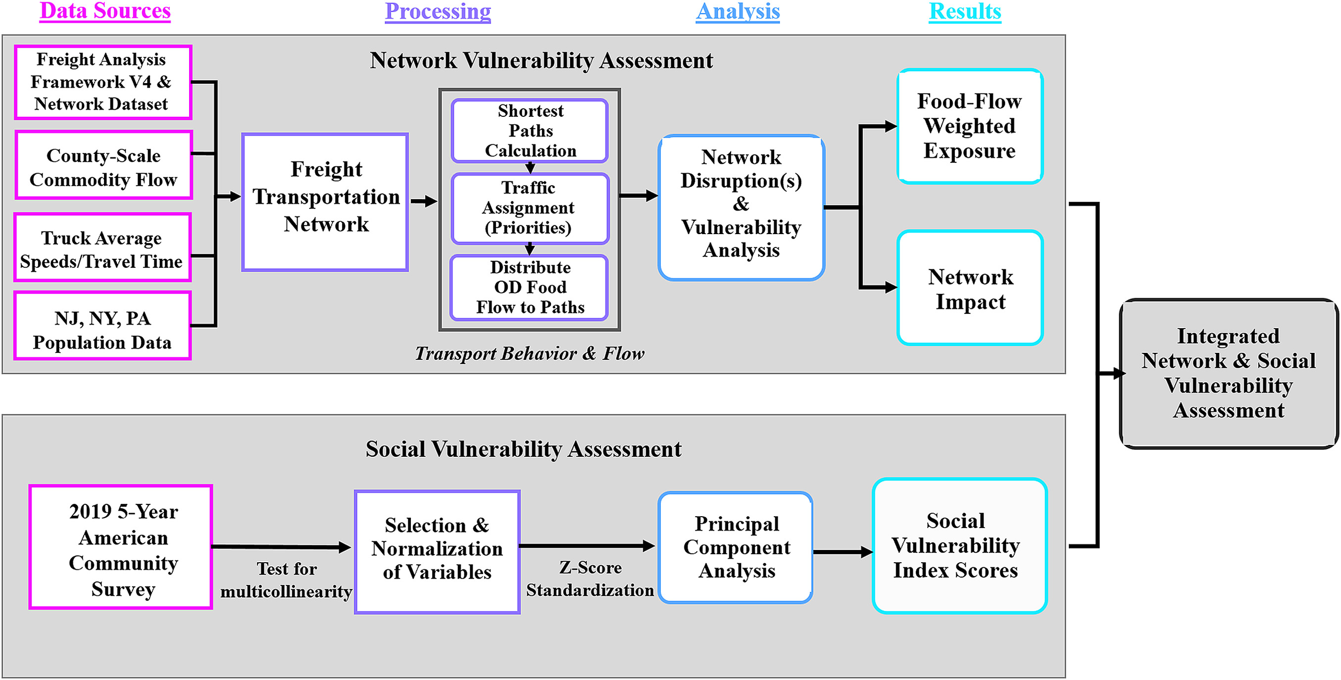
To leverage network science, transportation theory, and social vulnerability analysis to analyze our research questions around exposure, disruptions, and social vulnerability, we created a systems model combining existing data (Fig. 1). All data leveraged in this analysis are open source and available (see Supplemental Materials).
Study Area and Freight Transportation Network Creation
For this case study, the Mid-Atlantic region of the United States serves as an exploratory area of investigation. The three states considered are New Jersey, New York, and Pennsylvania. These states are home to 40.9 million people, which is about 13% of the US population. This region is of particular interest because it includes thousands of miles of key bridges, railroads, highways, and tunnels critical to the movement of goods and people countrywide.
We established the base roadway network using the national highway network data set of the Freight Analysis Framework (FAF) as a starting point. We selected the most populous cities [origins/destinations (ODs)] between the states as the center point for food commodity transportation in and out of the counties. The total city/county selection was 40 city/county pairs, nine in New Jersey, 15 in New York, and 16 in Pennsylvania. To reduce computational burdens but still retain sufficient redundancy, we took several steps to simplify the network. First, we selected major highways and local roads with greater than or equal to 20 trucks/road segment/day. We chose to simplify our network using truck volume because it created a mostly continuous network. Using other simplification techniques, such as speed limit or number of lanes or road type, the network was significantly disconnected, because speed limits and numbers of lanes may change suddenly.
We then aggregated the N-CAST travel time data set to the designated pathways. Disjointed road network segments were merged, and the network was planarized (adding nodes for intersections of crossing segments) and cleaned (removed unnecessary or dangling paths). Road segments near the boundaries of states to the closest intersection out of state were included if they were likely to be used for rerouting or deviation, so additional intersections in the states of Ohio, West Virginia, Maryland, and Delaware were also utilized. When N-CAST travel time data were not available, Google Maps data were used for road segments with missing travel time attributes.
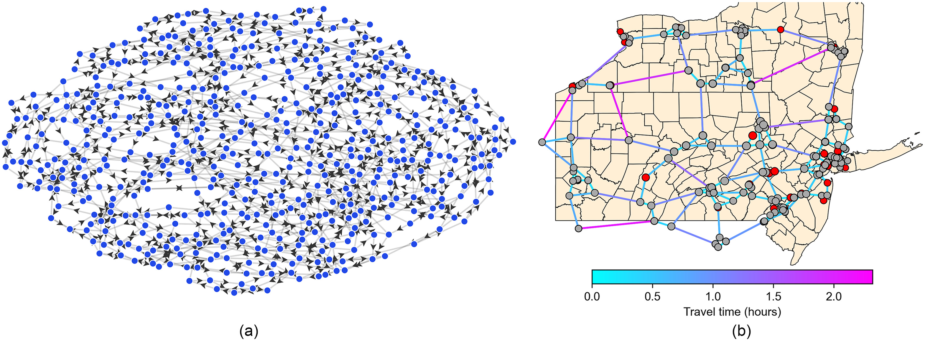
The final weighted and directed freight transportation network is illustrated in Fig. 2. The Mid-Atlantic freight transportation network consists of 509 nodes (40 centroid/county nodes, 469 intersections), 906 weighted edges [attributes: length (mi), average speed (mi/h), and travel time (h)], and 478 OD shortest paths (five per OD pair). In this exploratory analysis, we considered this Mid-Atlantic region as a closed system, thus we did not simulate traffic across the system boundaries.
Transport Behavior and Flow Assignment
To complete our network assignments, we calculated shortest paths, assigned traffic flows, and distributed food commodity flows to our network. We constrained the network to consider five shortest paths. Shortest paths were determined using existing probability formulas where the utility of a given route, , is a function of travel time on route and a standard time coefficient, , set to based on existing literature (Ding-Mastera 2016; Modesti and Sciomachen 1998)
(1)
The probability of choosing a route, , was defined in proportion to the whole choice set
(2)
Food flow was assigned to the network leveraging existing intranational commodity flows from the Federal Highway Administration’s (FHWA’s) FAF (Hwang et al. 2016). The OD FAF4 flows are provided at a coarse spatial resolution, so we leveraged the data-driven downscaled commodity flows for county-to-county origin and destinations for all seven food-related classes (SCTG 1-7) (Lin et al. 2019).
In our analysis, we considered five shortest paths as possible routes for county-level food transportation by truck. We chose to consider the five shortest paths for both computational minimization as well as following practices by a number of existing studies that determined five shortest paths was a viable analysis point for theoretical experiments in transport modeling behavior (Jha et al. 1998; Rahman et al. 2012; Shafiei et al. 2020; Zhu and Levinson 2015).
Social Vulnerability Index
To quantify vulnerability to commodity flow disruptions, we calculate a SoVI to understand the spatial variability of household food insecurity in New York, New Jersey, and Pennsylvania, and to determine the relationship social vulnerability may have correlating to commodity flow transportation disruptions. Our SoVI consists of 17 variables spanning four domains of race and ethnicity, economic status, housing composition, and housing type (Table 1) derived from county-level census data from the 2019 American Community Survey (US Census Bureau 2019). We selected this variable set based on existing literature that documents relationships between these socioeconomic indicators and vulnerability across food, water, and energy natural hazard research, thus representing important indicators relevant to material disruption in the food supply chain. For the theoretical justification grounding SoVI variable selection, see the Supplemental Materials.
| Domain | Variable No. | Description |
|---|---|---|
| Race and ethnicity | 1 | Percent Black or African American |
| 2 | Percent Hispanic or Latino | |
| 3 | Percentage of Alaska Native and American Indian Population | |
| Household composition | 4 | Percent of population under 18 years old |
| 5 | Percent of population over 65 years old | |
| 6 | Percent females | |
| 7 | Percent female-headed households, no spouse present | |
| 8 | Percent female-headed households, no spouse present, with children under 18 years | |
| 9 | Percent male-headed households, no spouse/partner present, with children under 18 years | |
| 10 | Percent female-headed households, no spouse present, living alone | |
| 11 | Percent male-headed households, no spouse present, living alone | |
| 12 | Percent of population with no high school diploma, 25 years and over | |
| 13 | Percent of civilian noninstitutionalized population with a disability | |
| Economic status | 14 | Percent living in poverty ( of the poverty level) |
| Household type | 15 | Percent of mobile home housing units |
| 16 | Percent multifamily housing units (five or more units) | |
| 17 | Percent of housing units built up to 1989 |
We began by testing for multicollinearity among the initial identified 19 variables, resulting in 17 variables. Then we normalized the selected variables using the total population and/or households of the respective county. The input variables were scaled and centered using -score standardization by subtracting by the mean and dividing by the standard deviation. Principal component analysis (PCA) was employed to calculate the social vulnerability scores and determine the dominant social factors. After performing PCA, five principal components (PCs) were identified based on the Kaiser selection criterion, which indicates an eigenvalue greater than 1. Overall, the five PCs describe approximately 79.3% of the variance. From the determination of the PCs, varimax rotation was implemented to understand the dominant social factors of the PCA output. The social factors were assigned factor names based on the theme of the principal variables, which were selected if the correlation was greater than (±) 0.50 (Table 2).
| Component name | Percent variance explained | Principal variables (± correlation) | Cardinality (effect of SoVI) |
|---|---|---|---|
| 1. Ethnicity, race, and multifamily housing | 27.5 | Hispanic or Latino () | + |
| Black or African American () | |||
| Multifamily housing () | |||
| Single female with children under 18 years old () | |||
| Older adults (over 65 years old) () | |||
| Female-headed households, no spouse present () | |||
| Mobile home housing () | |||
| 2. Education and low income | 17.9 | Education (no high school diploma) () | + |
| Income ( poverty level) () | |||
| Civilian noninstitutionalized population with a disability () | |||
| 3. Men and women living alone | 15.3 | Single female living alone () | + |
| Single male living alone () | |||
| Housing built before the year 1989 () | |||
| 4. Female and children | 10.8 | Female () | + |
| Children (under 18 years old) () | |||
| 5. American Indian and Alaska Native (AIAN) | 7.71 | American Indian and Alaska Native () | + |
| Single men with children under 18 years old () |
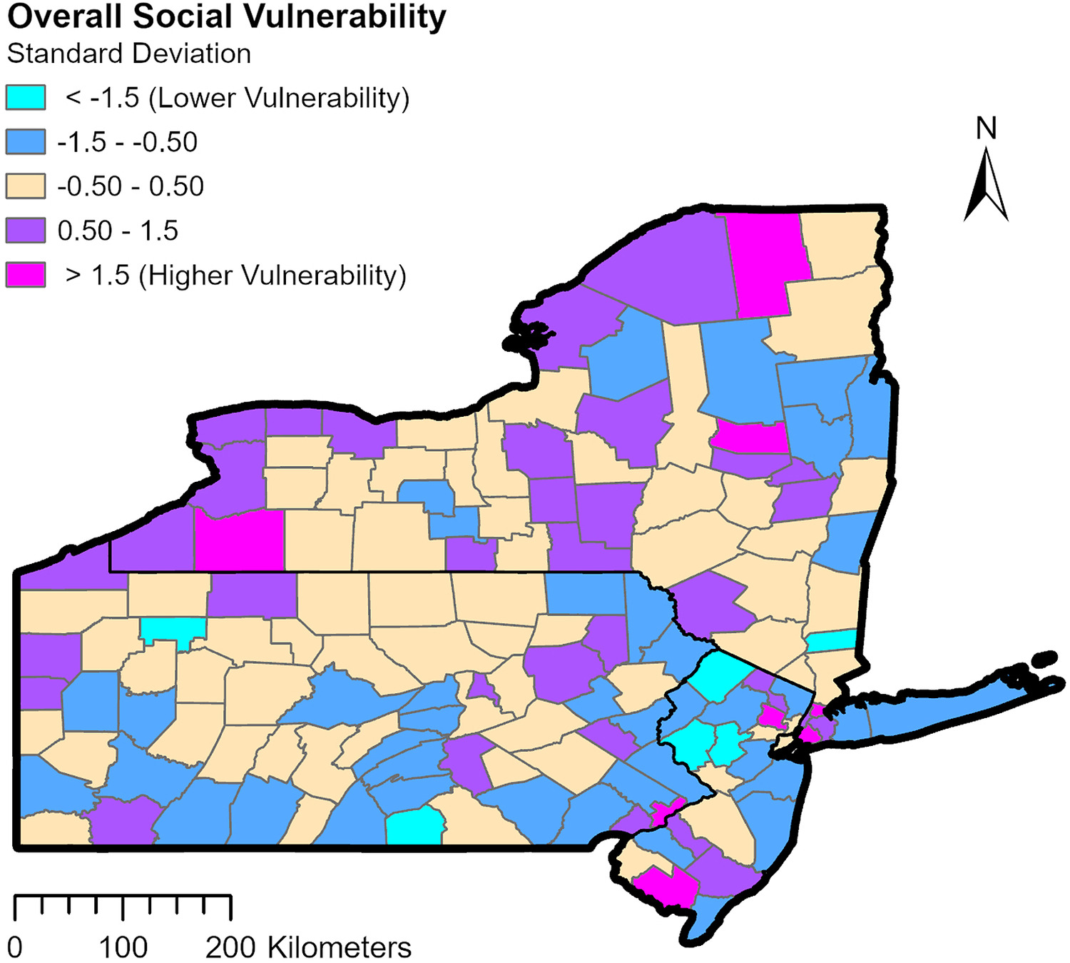
The five factor scores were then placed in an additive model to produce the composite social vulnerability score [Eq. (3)]. The factors were provided equal weighting given no defensible method for a weighting scheme (Cutter et al. 2003). Additionally, in SoVI construction, it is important to identify directionality with the principal variables (+, −). All variables increase vulnerability and are therefore added together. The summed overall SoVI factor scores were then spatially mapped into five divergent classes based on the standard deviation from the mean to highlight the most and least vulnerable block groups (BGs), ranging from (lower vulnerability) to (higher vulnerability)
(3)
Analysis of Network Impact and Exposure
In this study, we performed three phases of analysis. The first phase evaluated the system-level impact to the network in terms of performance due to both random and deterministic or targeted disruption. The second phase considered the exposure of each county’s food supply to disruptions in the network. The third phase analyzed whether there are relationships between social vulnerability and network exposure.
In Phase 1, we conducted our random disturbance analysis by selecting one node (or edge) at random, removing it from the network, and then measuring the impact on shortest paths and food flows. We repeated this process until we removed 40 nodes or edges. The choice of 40 node/edge removal was made for several reasons including computational efficiency, alignment with previous literature, and the presence of 40 city/county node pairs. Additionally, we chose not to focus on low-probability, high-intensity events that would disrupt far more than 40 nodes/edges because our food-flow data represent an annual time span. Thus, such low-probability, high-intensity events are unlikely to occur for the duration that matched the time scale of our food-flow data. To assess the average importance of different types of nodes (edges), we also assessed three cases: (1) removing any node (or edge) in the list, (2) removing only nodes (or edges) representing the locations of counties that are origins or destinations of food flows, and (3) removing only intersection nodes (or edges). To account for the uncertainty in the selection of the random node to be removed, we ran 1,000 realizations of this node removal process with different random nodes being removed in each realization. For the deterministic (i.e., targeted) disruptions of nodes (or edges) in the network, we selected nodes and edges using centrality-based indexes (Mattsson and Jenelius 2015; Zhang et al. 2015). The centrality-based metrics used here are betweenness centrality and closeness centrality (see Supplemental Materials for formal definition).
For the second phase of our analysis, we calculated the exposure (Jenelius et al. 2006; Rodríguez-Núñez and García-Palomares 2014) of counties to food-flow access due to disruptive events. This allowed us to determine how vulnerable counties are to disruptions in flood-flow access due to unexpected events. The standard indicator of accessibility for the user is the cost of travel. Thus, we employed the average travel time between OD pairs as a measure of travel cost and considered either the total food-inflow or food-outflow volume of each OD pair as the significant weight. First, we calculated the exposure of the county nodes by determining the average increase in travel time for trips starting (origin) or ending (destination) in the county () when a random node in the set of all nodes is disrupted. Then we multiplied this change in travel cost by the total food-inflow weight of the county node. This measurement is defined as the food-flow weighted exposure (FFWE), which helps us understand how disruption in the network affects a county’s access to food flow [Eq. (4)]
(4)
Finally, to bring the exploratory analysis to a close, for Phase 3 we investigated various relationships between SoVI and exposure across our study region. We investigated the relationship between inflow and outflow with SoVI as well as the relationship with SoVI and exposure across each of the five main dimensions.
Results
First, we present and discuss the results from the network response to disruptions analysis and the exposure of nodes to disruptions in the freight transportation network. Next, the social vulnerability of counties in the Mid-Atlantic region is investigated and discussed. Finally, we investigate freight transport–related inequalities in counties in the Mid-Atlantic region by looking at the intersection of the social vulnerability and exposure to food transportation disruptions of counties.
Because we considered five shortest paths as possible routes for county-level food transportation by truck, we assumed that the number of shortest paths or food transportation routes will be affected as a result of a node/edge removal, which in turn affects the capacity of the network to transport food commodities. Thus, the percentage of shortest paths after a node/edge removal describes the connectivity of the network, while the percentage of flows (by volume) indicates the strength of the network after the impact. Fig. 3 shows the difference between impacts to the network caused by random disruptions and deterministic attacks (centrality based and flow based). The impact to the network is shown both as a function of the percentage of shortest paths [Figs. 3(a and b)] and food flows [Figs. 3(c and b)] impacted after nodes and edges are removed from the network.
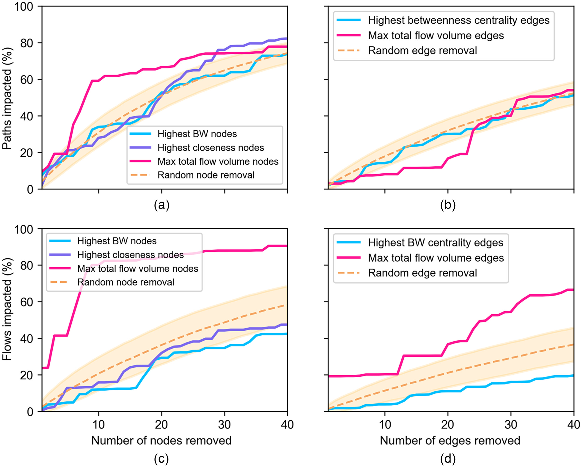
When we investigated connectivity, or the percent of paths impacted, we found that for the first 10 nodes removed, deterministic attacks based on closeness and betweenness centrality and maximum flow fell within the random range [Figs. 3(a and b)]. This means that in our network, targeted attacks are not more impactful than random removals when fewer nodes are removed. After the removal of nodes, we found that the attacks based on the maximum flow volume of nodes can produce higher impacts than random disruptions, whereas for centrality-based attacks the impacts are largely random. The curve representing removal of nodes with the highest betweenness centrality falls within the random range during the entire sequence of node removals. This suggests that betweenness centrality alone might not be suitable to assess connectivity in our transportation network. After nodes are removed, attacks based on closeness centrality hinder connectivity more than those based on maximum flow or random disruption [Fig. 3(a)]. This suggests that for a large number of nodes impacted, attacks based on closeness centrality hinder connectivity more than those based on maximum flow.
In our analysis of edge removal, we discovered that the impact on network connectivity is less significant than the impact of random edge removal when considering both betweenness centrality and maximum total flow [Fig. 3(b)]. This suggests that removing edges based on their centrality does not have as strong an impact on network connectivity as randomly removing edges. As expected, when examining the only county subset of nodes and edges during the random impact analysis, we found that their removal had a greater effect on connectivity compared to the removal of only intersection and all node/edge categories when removing nodes or edges one at a time (see Supplemental Materials). Additionally, in our network, removing nodes has a more substantial impact on connectivity than edge removal across all element types including any, only county, and only intersection (see Supplemental Materials).
Analysis of the disruptive scenarios reveals that the impact is much greater in the maximum total flow targeted attack than in the other centrality-based and random attacks. As previous authors have mentioned, the flow-based features of networks are not often considered in the literature, or when they are, they can be misrepresented due to weak estimates of function (Matisziw et al. 2009; Ouyang et al. 2014). Intuitively, connectivity is an important factor to understand when studying risk within networks, this assessment confirms that network flow, in our case, also shows an important component of risk assessment.
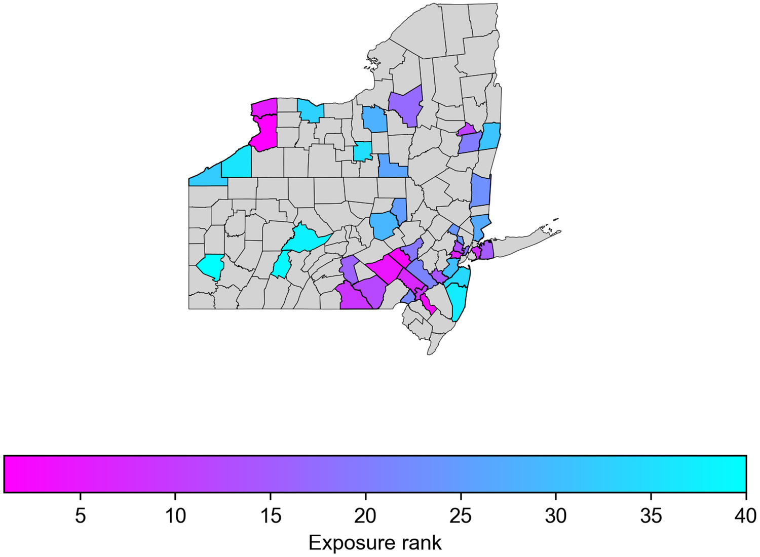
Our results also found that the counties with the highest food-weighted exposure ranking are generally located in the southeast of the region (Fig. 4). In our study area, a large portion of this exposure metric is attributed to the high demand for food inflow in the area (Fig. 6). Erie County (Buffalo), New York, situated in the northwestern part of the region, is the most susceptible county in terms of this food-weighted exposure metric. This county, located on the periphery of the network, has both a small number of connecting edges to the rest of the network and a high total amount of food inflow (Fig. 6). In contrast, the less exposed counties in the western region of Pennsylvania can maintain service and accessibility during disruptions, with their functionality remaining close to their original state. Hence, when nodes or edges are removed or not functioning in the network, the county food-flow exposure to disruptions will be lower in areas where more alternative routes are available. While one might expect that a higher number of intersections would reduce exposure, our results show no significant correlation between county exposure and the number of network nodes within the county.
Analyzing the spatial distribution of SoVI scores, we observe differences in social vulnerability between counties (Fig. 5). The map demonstrates that 4% of the total counties have a lower vulnerability ( standard deviation), 27% of the counties have a moderate to lower vulnerability ( to standard deviation), 42% of the counties have a moderate vulnerability ( to 0.5 standard deviation), 22% have a moderate to higher vulnerability (0.5 to 1.5 standard deviation), and 5% a have higher vulnerability ( standard deviation). Of the counties selected for the network analysis, Philadelphia County, Pennsylvania, and Essex County, New Jersey, have the highest overall social vulnerability, ranging between 0.5 and 1.5 times the standard deviation.
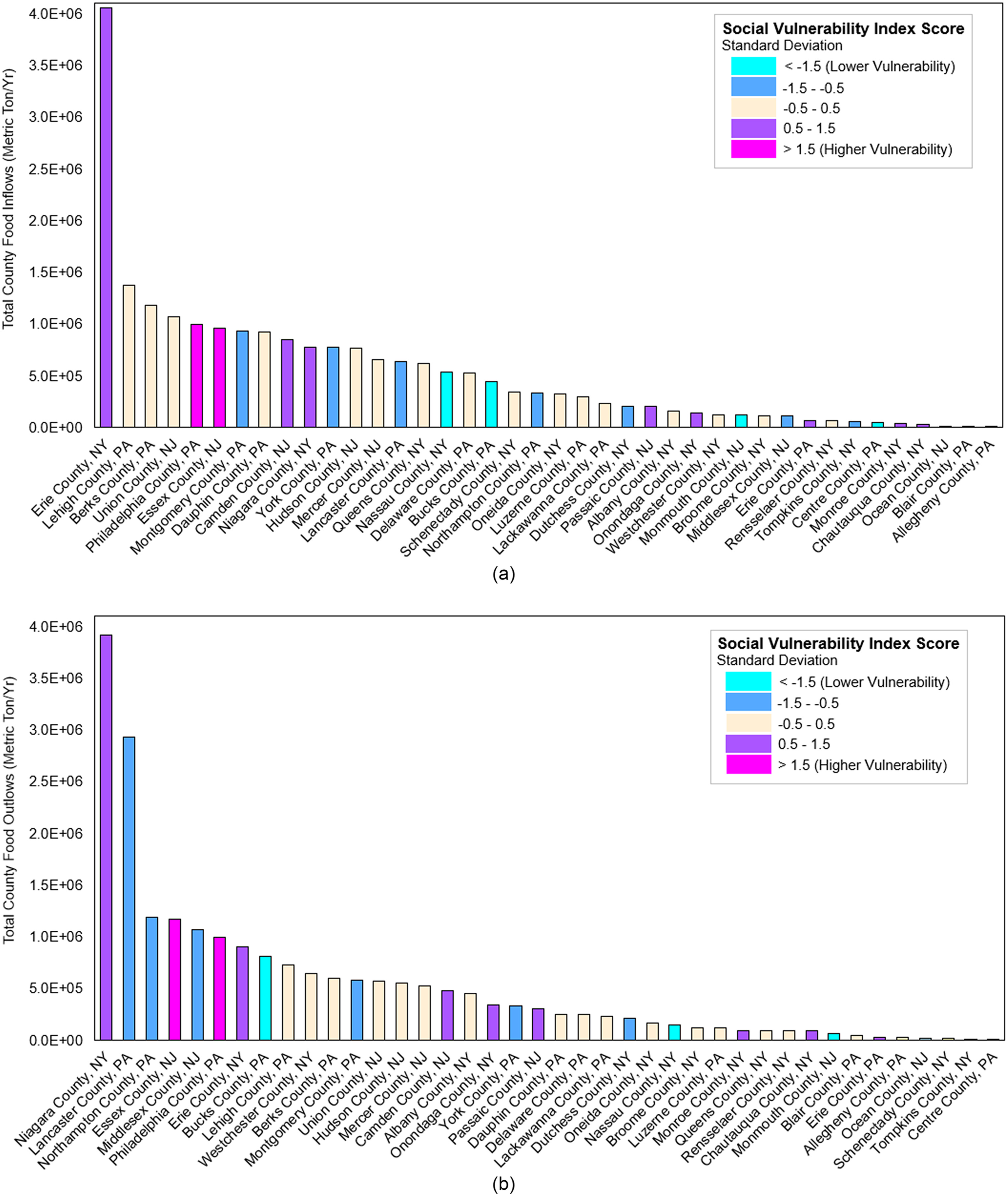
For the total county food-flow plots, we see some variability among the county’s total flow and social vulnerability index score (i.e., flow and SoVI value do not have the same trends). Fig. 6(a) demonstrates that some locations have both high food flows and high vulnerability. For example, Erie County, New York, has the highest inflow value () and a moderate to high social vulnerability (0.5–1.5 standard deviation). The most socially vulnerable counties ( standard deviation), Philadelphia County, Pennsylvania, and Essex County, New Jersey, have total inflow values of and , respectively ( and ). From Fig. 7, Niagara County, New York, has the most outflow () and a moderate to high social vulnerability (0.5–1.5 standard deviation). Lehigh County follows with a total inflow of and with a moderate social vulnerability, and Lancaster County, Pennsylvania, with a total outflow of and low to moderate vulnerability ( to standard deviation).
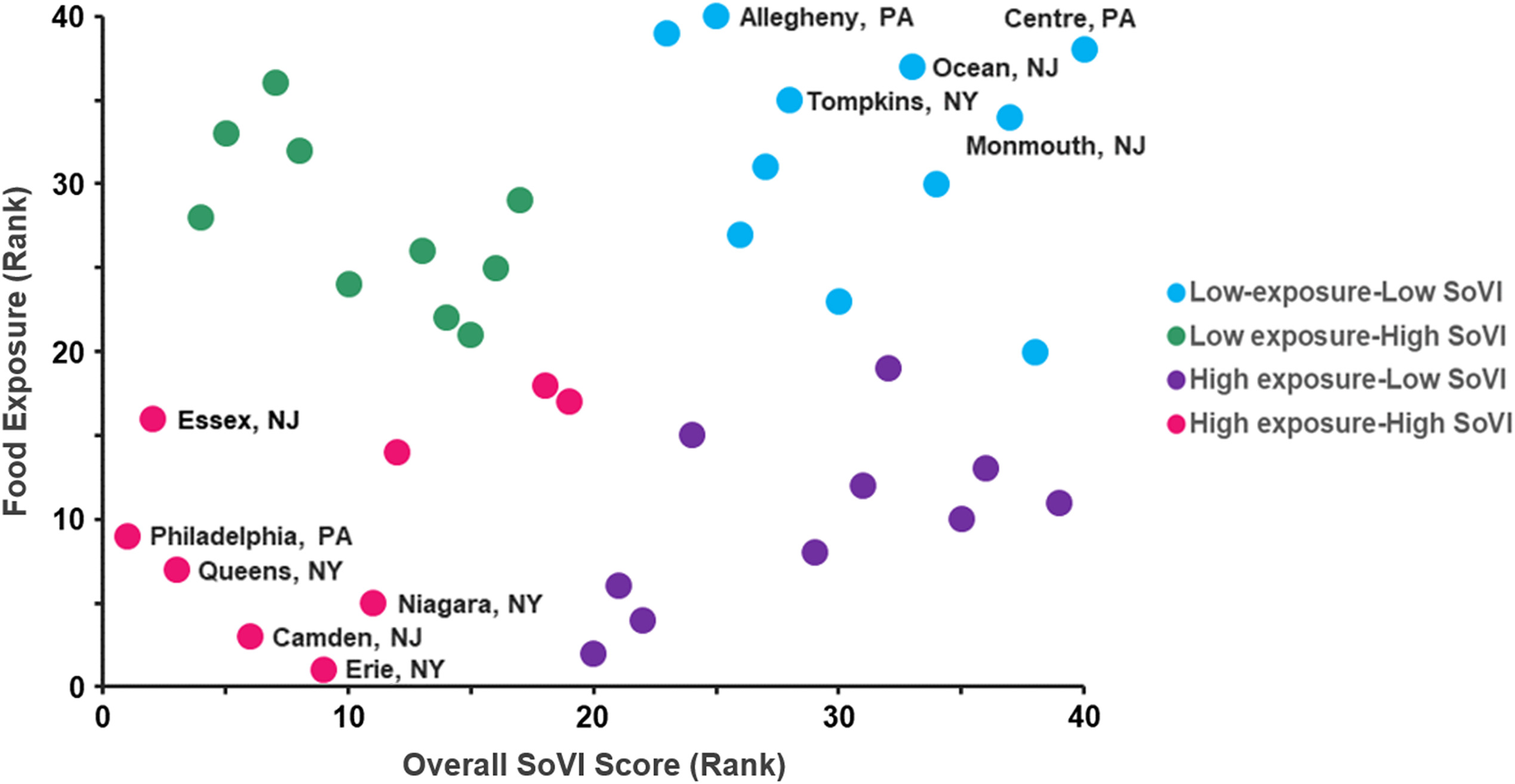
Vulnerability to disruptions is not only determined by the potential physical network failures, but also by the capability of communities to withstand unprecedented events. To further test vulnerability by exploring both disruption impacts and the capability of communities to withstand them, we show a scatterplot of food-weighted exposure versus SoVI ranking for the 40 network-defined counties in Fig. 7. To distinguish these communities we can view quadrants based on high and low exposure and vulnerability ranks. Quadrant 1, in the bottom left side of the scatter, includes the high exposure–high SoVI category, which is composed by the top counties with exposure and vulnerability ranks below 20. Quadrant 2, high exposure–low SoVI, consists of counties with an exposure rank 1–20 and SoVI rank 21–40. Quadrant 3, low exposure–high SoVI, includes counties with an exposure rank greater than 20 and a SoVI rank of 20 or less. Last, low exposure–low SoVI is classified as counties with a food-flow exposure and SoVI ranking greater than 20. Both Figs. 7 and 8 suggest no significant linear correlation but can still highlight vulnerable regions where additional resources might be necessary. Counties with high exposure–high SoVI include Essex County and Camden County, New Jersey; Erie County, Niagara County, and Queens, New York; and Philadelphia County, Pennsylvania. These areas could be particularly vulnerable in scenarios where critical transportation routes are disrupted and highlight areas where planning and investment in infrastructure and hazard mitigation could protect vulnerable communities. Counties with low exposure–low SoVI include Monmouth County and Ocean County, New Jersey; Tompkins County, New York; and Allegheny County and Centre County, Pennsylvania.
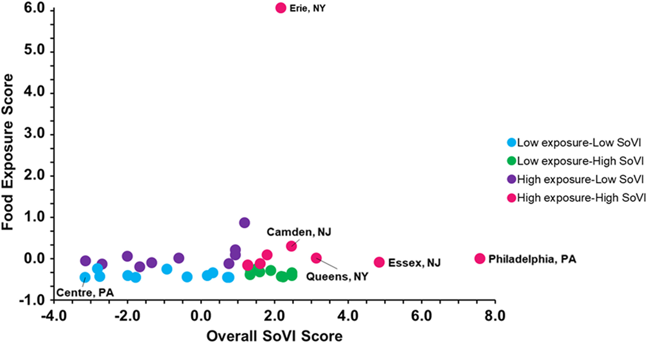
Examining food-weighted exposure and SoVI in more detail, Fig. 8 compares standard score values for the 40 network-defined counties. From this scatterplot we can see how counties are now grouped close together and recognize the gap between vulnerability categories. Additionally, we can spot a few outliers that set apart from the rest, for example, Erie County, New York; Philadelphia County, Pennsylvania; and Essex County, New Jersey.
Discussion and Limitations
Integrating and comparing the counties for both network exposure and SoVI provides a transformative framework that highlights the ways that social vulnerability interacts with disruption to transportation infrastructure and access to goods. This framework can be applied to other or larger areas and scenarios, and this type of analysis could provide decision makers with a more holistic view into how actions to protect transportation infrastructure like road retrofitting and protection, as well as emergency response, could take into account the social vulnerability of communities that are impacted.
Advances in data availability would strengthen future work in this area. There were some limitations in this study, data availability being the main one. In this study, our analysis was constrained to the county scale because this was the smallest scale of commodity flow data available. If data were available below the county scale, the transportation network and subsequent disruption analysis could be conducted in greater detail, which would allow for better characterization of the impacts on communities. Additionally, we used yearly commodity flow data. Thus, the amounts of food flow disrupted are for theoretical comparisons only because disruption most often occurs on a much smaller timescale. Despite these limitations, we believe the framework presented in this exploratory research that investigates theoretical interconnections and addresses ethical implications in transportation disruption analysis is a useful first step in this research.
Another important implication of our methodological choices revolves around the simplification of the road network. We removed roads that were not transited by trucks per day, which removed many tertiary roads. In reality, these tertiary roads may indeed serve connectivity needs when major routes are blocked. Thus, future analyses could expand the complexity of our network to consider all possible routing behaviors. Additionally, restricting movement to five shortest paths could be unbounded for future analyses allowing for more path routing possibilities. We also studied the removal of 40 nodes/edges due to computational efficiency, previous literature, and the presence of 40 city/county node pairs. In reality, however, there may be low-probability, high-intensity events that exceed the 40 node/edge removal. We chose not to study these extremely low-probability events because our food-flow data represent an annual volume and such events do not last for such a long period of disruption. Future work in the emergency management space could adapt our methodological approach to study such disruptions with access to real-time or shorter time duration data on food flows.
An organic future step is to expand the road network to include all US counties. Additionally, incorporating other freight commodities, such as industrial commodities, would allow for analysis beyond food systems. However, to do so, we must produce data sets of industrial commodities at a finer spatial scale. Further, this network disruption analysis could be expanded by including different infrastructure types in a multilayer network framework. For example, other infrastructure types to consider could include other modes of transportation (e.g., rail, water, air), agricultural and industrial products processing plants, retailers, electricity generation infrastructure, and water treatment plants. This critical infrastructure network could simulate more real-world disturbances such as floods, drought, and hurricanes.
The implications of this work could help practitioners discover critical locations that influence disruption to food-flow commodities due to road network perturbations. These areas could be prioritized for transportation planning so that the critical routes, roads, and/or intersections are prioritized for hazard mitigation and protection. Identification of communities that are vulnerable to access loss to food, water, and energy resources could allow managers to promote the inclusion of people’s needs in the relief and resource allocation siting decision-making. Discovering the most vulnerable communities could inform emergency response planning or those who wish to prioritize resource allocations among certain communities to reduce the societal impact of the loss of accessibility. However, there is still work to be done on what stakeholders are responsible for mitigating disruption risks and protecting human well-being (Grady et al. 2021).
Conclusions
Understanding the impact of disruptions on different communities is crucial for analyzing the sustainability and equity of infrastructure systems. This study combined a county-level social vulnerability assessment with transportation network analysis to better comprehend the effects of disruption and to inform decisions that can allocate resources and assistance to the most vulnerable areas. This research identified the overall network impacts due to disruptions and highlighted the most exposed counties, which are more susceptible to food-flow commodity disruptions based on their position within the network. By utilizing a social vulnerability index, this study demonstrated how different communities experience hardships and pinpointed areas with socially vulnerable populations. The comparison of network vulnerability and SoVI helped identify the most at-risk communities to inform emergency response planning. Prioritizing these areas for resource allocation could help minimize the societal impact of accessibility loss.
To conclude, integrating social equity dimensions into transportation planning is just one step toward a more comprehensive approach. Including social vulnerability in transportation and commodity flow studies is essential for promoting equitable transportation planning and hazard mitigation. Further research in this area is necessary to support policymakers and planners in creating systems that serve all.
Supplemental Materials
File (supplemental materials_jitse4.iseng-2258_delgado.pdf)
- Download
- 2.00 MB
Data Availability Statement
All data, models, or code that support the findings of this study are available from the corresponding author upon reasonable request. All of the constructed databases were formed using open and available public information as indicated throughout the methods and Supplemental Materials.
Acknowledgments
The authors would like to acknowledge the National Science Foundation Grants Nos. 1941657 and 2244715 for providing support for this work. Author C. Grady is the sole PI for Grant Nos. 1941657 and 2244715. This grant also supported authors L. Delgado and S. Hinojos. The authors would also like to thank Vikash Gayah and Ilgin Gueller for their helpful suggestions.
References
Ahmed, Q. I., H. Lu, and S. Ye. 2008. “Urban transportation and equity: A case study of Beijing and Karachi.” Transp. Res. Part A: Policy Pract. 42 (1): 125–139. https://doi.org/10.1016/j.tra.2007.06.004.
Balakrishnan, S., and Z. Zhang. 2018. “Developing priority index for managing utility disruptions in urban areas with focus on cascading and interdependent effects.” Transp. Res. Rec. 2672 (1): 101–112. https://doi.org/10.1177/0361198118774239.
Bellamy, M. A., and R. C. Basole. 2013. “Network analysis of supply chain systems: A systematic review and future research.” Syst. Eng. 16 (2): 235–249. https://doi.org/10.1002/sys.21238.
Boyle, E., A. Inanlouganji, T. Carvalhaes, P. Jevtic, G. Pedrielli, and T. A. Reddy. 2022. “Social vulnerability and power loss mitigation: A case study of Puerto Rico.” Int. J. Disaster Risk Reduct. 82 (Nov): 103357. https://doi.org/10.1016/j.ijdrr.2022.103357.
Cutter, S. L. 2017. “The perilous nature of food supplies: Natural hazards, social vulnerability, and disaster resilience.” Environ.: Sci. Policy Sustainable Dev. 59 (1): 4–15. https://doi.org/10.1080/00139157.2017.1252603.
Cutter, S. L., L. Barnes, M. Berry, C. Burton, E. Evans, E. Tate, and J. Webb. 2008. “A place-based model for understanding community resilience to natural disasters.” Global Environ. Change 18 (4): 598–606. https://doi.org/10.1016/j.gloenvcha.2008.07.013.
Cutter, S. L., B. J. Boruff, and W. L. Shirley. 2003. “Social vulnerability to environmental hazards.” Social Sci. Q. 84 (2): 242–261. https://doi.org/10.1111/1540-6237.8402002.
Demirel, H., M. Kompil, and F. Nemry. 2015. “A framework to analyze the vulnerability of European road networks due to sea-level rise (SLR) and sea storm surges.” Transp. Res. Part A: Policy Pract. 81 (Nov): 62–76. https://doi.org/10.1016/j.tra.2015.05.002.
Ding-Mastera, J. 2016. “Adaptive route choice in stochastic time-dependent networks: Routing algorithms and choice modeling.” Doctoral dissertation, Dept. of Civil Engineering, Univ. of Massachusetts Amherst.
Dong, S., A. Esmalian, H. Farahmand, and A. Mostafavi. 2020. “An integrated physical-social analysis of disrupted access to critical facilities and community service-loss tolerance in urban flooding.” Comput. Environ. Urban Syst. 80 (Mar): 101443. https://doi.org/10.1016/j.compenvurbsys.2019.101443.
Eid, M. S., and I. H. El-adaway. 2017. “Integrating the social vulnerability of host communities and the objective functions of associated stakeholders during disaster recovery processes using agent-based modeling.” J. Comput. Civ. Eng. 31 (5): 04017030. https://doi.org/10.1061/(ASCE)CP.1943-5487.0000680.
Executive Office of the President. 2021a. “Executive Order 13985: Advancing racial equity and support for underserved communities through the federal government.” Fed. Regist. 86 (14): 7009–7013.
Executive Office of the President. 2021b. “Executive order 14017: America’s supply chains.” Fed. Regist. 86 (38): 11849–11854.
Faturechi, R., and E. Miller-Hooks. 2015. “Measuring the performance of transportation infrastructure systems in disasters: A comprehensive review.” J. Infrastruct. Syst. 21 (1): 04014025. https://doi.org/10.1061/(ASCE)IS.1943-555X.0000212.
FEMA. 2022. “Equity.” Accessed August 3, 2022. https://www.fema.gov/emergency-managers/national-preparedness/equity.
Garschagen, M., and S. Sandholz. 2018. “The role of minimum supply and social vulnerability assessment for governing critical infrastructure failure: Current gaps and future agenda.” Nat. Hazards Earth Syst. Sci. 18 (4): 1233–1246. https://doi.org/10.5194/nhess-18-1233-2018.
Gomez, M., S. Garcia, S. Rajtmajer, C. Grady, and A. Mejia. 2020. “Fragility of a multilayer network of international supply chains.” Appl. Network Sci. 5 (1): 71. https://doi.org/10.1007/s41109-020-00310-1.
Grady, C. A., S. Rajtmajer, and L. Dennis. 2021. “When smart systems fail: The ethics of cyber–physical critical infrastructure risk.” IEEE Trans. Technol. Soc. 2 (1): 6–14. https://doi.org/10.1109/TTS.2021.3058605.
Gralla, E., J. Goentzel, and C. Fine. 2014. “Assessing trade-offs among multiple objectives for humanitarian aid delivery using expert preferences.” Prod. Oper. Manage. 23 (6): 978–989. https://doi.org/10.1111/poms.12110.
Huang, M., K. Smilowitz, and B. Balcik. 2011. “Models for relief routing: Equity, efficiency and efficacy.” Procedia - Social Behav. Sci. 17 (1): 416–437. https://doi.org/10.1016/j.sbspro.2011.04.525.
Hwang, H.-L., S. Hargrove, S.-M. Chin, D. W. Wilson, H. Lim, J. Chen, R. Taylor, B. Peterson, and D. Davidson. 2016. The freight analysis framework version 4 (FAF4)—Building the FAF4 regional database: Data sources and estimation methodologies. Oak Ridge, TN: Oak Ridge National Lab.
Jafino, B. A. 2021. “An equity-based transport network criticality analysis.” Transp. Res. Part A: Policy Pract. 144 (Feb): 204–221. https://doi.org/10.1016/j.tra.2020.12.013.
Jansuwan, S., A. Chen, and X. Xu. 2021. “Analysis of freight transportation network redundancy: An application to Utah’s bi-modal network for transporting coal.” Transp. Res. Part A: Policy Pract. 151 (Sep): 154–171. https://doi.org/10.1016/j.tra.2021.06.019.
Jenelius, E., T. Petersen, and L.-G. Mattsson. 2006. “Importance and exposure in road network vulnerability analysis.” Transp. Res. Part A: Policy Pract. 40 (7): 537–560. https://doi.org/10.1016/j.tra.2005.11.003.
Jha, M., S. Madanat, and S. Peeta. 1998. “Perception updating and day-to-day travel choice dynamics in traffic networks with information provision.” Transp. Res. Part C: Emerging Technol. 6 (3): 189–212. https://doi.org/10.1016/S0968-090X(98)00015-1.
Karakoc, D. B., K. Barker, C. W. Zobel, and Y. Almoghathawi. 2020. “Social vulnerability and equity perspectives on interdependent infrastructure network component importance.” Sustainable Cities Soc. 57 (Jun): 102072. https://doi.org/10.1016/j.scs.2020.102072.
Lin, X., Q. Dang, and M. Konar. 2014. “A network analysis of food flows within the United States of America.” Environ. Sci. Technol. 48 (10): 5439–5447. https://doi.org/10.1021/es500471d.
Lin, X., P. Ruess, L. Marston, and M. Konar. 2019. “Food flows between counties in the United States.” Environ. Res. Lett. 14 (8): 084011. https://doi.org/10.1088/1748-9326/ab29ae.
Lobban, H., Y. Almoghathawi, N. Morshedlou, and K. Barker. 2021. “Community vulnerability perspective on robust protection planning in interdependent infrastructure networks.” Proc. Inst. Mech. Eng., Part O: J. Risk Reliab. 235 (5): 798–813. https://doi.org/10.1177/1748006X21991038.
Manaugh, K., and A. M. El-Geneidy. 2012. “Who benefits from new transportation infrastructure? Using accessibility measures to evaluate social equity in transit provision.” In Accessibility and transport planning: Challenges for Europe and North America, 221–227. London: Edward Elgar.
Matisziw, T. C., A. T. Murray, and T. H. Grubesic. 2009. “Exploring the vulnerability of network infrastructure to disruption.” Ann. Reg. Sci. 43 (2): 307–321. https://doi.org/10.1007/s00168-008-0235-x.
Mattsson, L.-G., and E. Jenelius. 2015. “Vulnerability and resilience of transport systems—A discussion of recent research.” Transp. Res. Part A: Policy Pract. 81 (Mar): 16–34. https://doi.org/10.1016/j.tra.2015.06.002.
Merschman, E., M. Doustmohammadi, A. M. Salman, and M. Anderson. 2020. “Postdisaster decision framework for bridge repair prioritization to improve road network resilience.” Transp. Res. Rec. 2674 (3): 81–92. https://doi.org/10.1177/0361198120908870.
Miller-Hooks, E., X. Zhang, and R. Faturechi. 2012. “Measuring and maximizing resilience of freight transportation networks.” Comput. Oper. Res. 39 (7): 1633–1643. https://doi.org/10.1016/j.cor.2011.09.017.
Modesti, P., and A. Sciomachen. 1998. “A utility measure for finding multiobjective shortest paths in urban multimodal transportation networks.” Eur. J. Oper. Res. 111 (3): 495–508. https://doi.org/10.1016/S0377-2217(97)00376-7.
Morrow, B. H. 1999. “Identifying and mapping community vulnerability.” Disasters 23 (1): 1–18. https://doi.org/10.1111/1467-7717.00102.
Nelson, A., S. Lindbergh, L. Stephenson, J. Halpern, F. A. Arroyo, X. Espinet, and M. C. González. 2019. “Coupling natural hazard estimates with road network analysis to assess vulnerability and risk: Case study of Freetown (Sierra Leone).” Transp. Res. Rec. 2673 (8): 11–24. https://doi.org/10.1177/0361198118822272.
Novak, D. C., J. F. Sullivan, K. Sentoff, and J. Dowds. 2020. “A framework to guide strategic disinvestment in roadway infrastructure considering social vulnerability.” Transp. Res. Part A: Policy Pract. 132 (Feb): 436–451. https://doi.org/10.1016/j.tra.2019.11.021.
Ouyang, M. 2014. “Review on modeling and simulation of interdependent critical infrastructure systems.” Reliab. Eng. Syst. Saf. 121 (Jan): 43–60. https://doi.org/10.1016/j.ress.2013.06.040.
Ouyang, M., L. Zhao, L. Hong, and Z. Pan. 2014. “Comparisons of complex network based models and real train flow model to analyze Chinese railway vulnerability.” Reliab. Eng. Syst. Saf. 123 (Mar): 38–46. https://doi.org/10.1016/j.ress.2013.10.003.
Papilloud, T., V. Röthlisberger, S. Loreti, and M. Keiler. 2020. “Flood exposure analysis of road infrastructure—Comparison of different methods at national level.” Int. J. Disaster Risk Reduct. 47 (Aug): 101548. https://doi.org/10.1016/j.ijdrr.2020.101548.
Paton, D., J. Mcclure, and P. Buergelt. 2006. “Natural hazard resilience: The role of individual and household preparedness.” In Disaster resilience an integrated approach, edited by D. Paton and D. Johnston, 105–127. Springfield, IL: Charles C Thomas Publisher.
Pereira, R. H. M., T. Schwanen, and D. Banister. 2017. “Distributive justice and equity in transportation.” Transp. Rev. 37 (2): 170–191. https://doi.org/10.1080/01441647.2016.1257660.
Rahman, A., N. E. Lownes, J. N. Ivan, L. Fiondella, S. Rajasekaran, and R. Ammar. 2012. “A game theory approach to identify alternative regulatory frameworks for hazardous materials routing.” In Proc., IEEE Conf. on Technologies for Homeland Security (HST), 489–494. New York: IEEE.
Reggiani, A., P. Nijkamp, and D. Lanzi. 2015. “Transport resilience and vulnerability: The role of connectivity.” Transp. Res. Part A: Policy Pract. 81 (Nov): 4–15. https://doi.org/10.1016/j.tra.2014.12.012.
Reid, J., and D. Wood. 2022. “Systems engineering applied to urban planning and development: A review and research agenda.” Syst. Eng. 26 (1): 88–103. https://doi.org/10.1002/sys.21642.
Rodríguez-Núñez, E., and J. C. García-Palomares. 2014. “Measuring the vulnerability of public transport networks.” J. Transp. Geogr. 35 (Feb): 50–63. https://doi.org/10.1016/j.jtrangeo.2014.01.008.
Shafiei, S., A.-S. Mihaita, H. Nguyen, C. Bentley, and C. Cai. 2020. “Short-term traffic prediction under non-recurrent incident conditions integrating data-driven models and traffic simulation.” In Proc., Transportation Research Board 99th Annual Meeting. Washington, DC: Transportation Research Record.
Tahmasbi, B., H. Haghshenas, and S. Birzhandi. 2021. “Network vulnerability analysis based on the overall and inequity impacts of the distribution of the added travel time to the network users.” Eur. J. Transp. Infrastruct. Res. 21 (1): 94–114. https://doi.org/10.18757/EJTIR.2021.21.1.5363.
Tierney, K. 2009. Disaster response: Research findings and their implications for resilience measures. Boulder, CO: Univ. of Colorado Boulder.
US Census Bureau. 2019. “American community survey data.” Accessed October 4, 2022. https://www.census.gov/programs-surveys/acs/data.html.
Zhang, X., E. Miller-Hooks, and K. Denny. 2015. “Assessing the role of network topology in transportation network resilience.” J. Transp. Geogr. 46 (Feb): 35–45. https://doi.org/10.1016/j.jtrangeo.2015.05.006.
Zhu, S., and D. Levinson. 2015. “Do people use the shortest path? An empirical test of Wardrop’s first principle.” PLoS One 10 (8): e0134322. https://doi.org/10.1371/journal.pone.0134322.
Information & Authors
Information
Published In
Journal of Infrastructure Systems
Volume 29 • Issue 4 • December 2023
Copyright
This work is made available under the terms of the Creative Commons Attribution 4.0 International license, https://creativecommons.org/licenses/by/4.0/.
History
Received: Oct 5, 2022
Accepted: May 30, 2023
Published online: Aug 4, 2023
Published in print: Dec 1, 2023
Discussion open until: Jan 4, 2024
Authors
Metrics & Citations
Metrics
Citations
Download citation
If you have the appropriate software installed, you can download article citation data to the citation manager of your choice. Simply select your manager software from the list below and click Download.