Space-Time Pressure Distribution Applied to a Stiff Concrete Structure through a Protective Sand Layer from Full-Scale Experimental Rockfall Tests

Garcia, Bruna; Oussalah, Tarik; Rajot, Jean-Pierre; Colas, Anne-Sophie

doi:10.1061/JGGEFK.GTENG-11787

Open access

Technical Papers

Feb 7, 2024

Space-Time Pressure Distribution Applied to a Stiff Concrete Structure through a Protective Sand Layer from Full-Scale Experimental Rockfall Tests

Authors: Bruna Garcia https://orcid.org/0000-0002-6547-9564 [email protected], Tarik Oussalah [email protected], Jean-Pierre Rajot https://orcid.org/0000-0003-1535-3944 [email protected], and Anne-Sophie Colas [email protected]Author Affiliations

Publication: Journal of Geotechnical and Geoenvironmental Engineering

Volume 150, Issue 4

https://doi.org/10.1061/JGGEFK.GTENG-11787

PDF

Abstract

This study focuses on the characterization of low-velocity (lower than

100 km / h

) rockfall impact loads transferring to a thick steel-reinforced concrete (SRC) slab through a protective sand layer. A full-scale experimental test campaign was performed, where each test consisted of releasing a concrete block which, after a vertical free fall, impacts a sand protective layer placed over a SRC slab, in order to represent an isolated rockfall impact to which an actual SRC structure could be exposed. During the impact, the vertical pressure distribution was observed using several pressure cells installed at the sand–slab interface. A total of 35 tests were carried out, systematically combining sand layer thickness (

D

), block’s equivalent diameter (

B

), and free-fall drop height (

H

), related to impact velocity. The masses of the released blocks were in the range of 117 to 7,399 kg, corresponding to diameters in the range of 0.42 to 1.79 m. Five free-fall drop heights up to 33 m were considered to reach impact velocities up to

90 km / h

, covering the range of most velocities observed in actual rockfall studies. Three thicknesses of the sand layer protecting the thick SRC slab were considered: 1, 1.5, or 2 m. Data reduction from this full-scale impact tests program makes it possible to characterize, for a given thickness of protective sand layer, the time-space pressure pulse distribution applied to the protected structure during the impact for a large range of rock boulder masses and speeds actually observed in the field.

Introduction

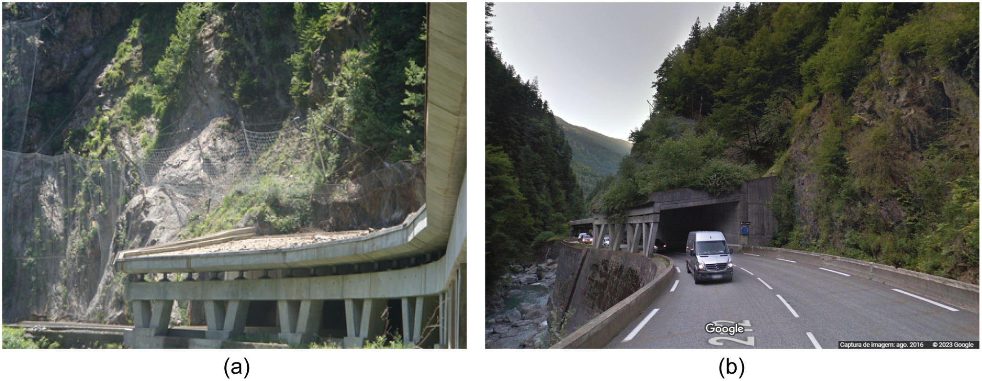
Among the possible rockfall protections, various types of steel mesh devices have been developed to mitigate rockfalls of low to medium impact energy (1 to 10 MJ). Rockfall shed galleries (Fig. 1) or, when adapted to the site profile, reinforced soil bunds are being used for medium to large energy levels. To improve the durability and maintenance of these structures, which are often critical for infrastructure operation and rescue organization, granular soil layers may be placed on the roof of rock-shed galleries, tunnel heads, or other structural elements possibly exposed to a direct hit from a falling rock boulder.

Fig. 1. (a) Example of a rock shed gallery in Val d’Arly (Ugine, French Alps) (image courtesy of Risque Rocheux et Ouvrages Géotechniques Laboratory of The Gustave Eiffel University); and (b) view of the rock shed (image ©2023 Google).

Granular soils are often available and their performance to protect structures from rockfall impacts, although not yet fully quantified, has been demonstrated for ages. Without a protective granular soil layer, the collision with the rock boulder produces significant damages to the steel-reinforced concrete structure to dissipate a large amount of energy within a very short period of time (Durville et al. 2010). When a soil layer is protecting the structure, large deformations and displacements occur in the soil during the impact, which dissipates part of the energy. The impact load is then transmitted to a wider surface of the structure and is applied more progressively and during a longer period, resulting in a lower damage to the structure.

In fact, analysis of the dynamic penetration of a rock boulder in soils, eventually with subsequent soil–structure interaction during penetration, raises several major issues for predictive numerical modeling. As a consequence, many authors rather developed experimental approaches to investigate the physical phenomena and propose empirical relationships. In the literature, a significant number of reduced-scale tests have been performed to investigate the influence of several factors, such as the block mass, block shape, impact velocity, angle of impact, protective soil grain size distribution, relative density, thickness of the layer, and so on. The majority of analytical or empirical expressions derived from these tests give an estimate of the maximum impact force at the top of the protective soil layer, but not to the force transmitted to the structure at the soil–slab interface.

Based on their reduced scale tests, some authors (Yoshida et al. 1988; Montani Stoffel 1998; Heidenreich 2004; Calvetti and Di Prisco 2012; Schellenberg 2008) proposed empirical relationships to estimate the maximum value of the impact force and the block’s penetration depth. They also considered the maximum value of the forces transmitted to the protected structure and to its foundation, which may differ from each other due to structural dynamic effects during impact. Other research results on dynamic structural design remain confidential due to private-company-led research or their potential military use.

Two of the most important design guidelines for rockfall protective soil layers are the Japanese Rockfall Countermeasures Handbook (Japan Road Association 2000) and the Swiss Technical Guide (ASTRA–Swiss Federal Transportation Office 2008). Based on the empirical relationships for the maximum value of the impact force and for the block penetration depth, these guidelines suggest recommendations to define the equivalent pressure distribution transferred through the protective layer to be considered in quasi-static design analysis of the structure. These guidelines also include requirements on the layer thickness to prevent the rock boulder from reaching the structure during an impact.

Still, several authors (Bhatti 2015; Pichler et al. 2005; Labiouse et al. 1996; Schellenberg 2008; Calvetti and Vecchiotti 2005; Kishi et al. 2002) pointed out the lack of full-scale tests to extrapolate these empirical expressions to actual rock block sizes and impact energies of the order of those observed in the field. In fact, in dynamics, inertia forces involve both the space scale and time scale, which therefore does not allow a unique similarity relationship to be defined between reduced-scale tests and the full-scale impacts in the field. Furthermore, for dynamic mechanical analysis of the protected structure, not only an equivalent quasi-static maximum value of the load transferred to the structure through the soil layer is needed, but the time rate and duration of the loading, as well as its spatial distribution, are of crucial importance because the inertia of the structure has a significant influence on the stress values actually applied to its constitutive materials during impact.

The main objective of the present study is to propose a method to characterize the space-time pressure pulse distribution applied to a structure protected by a sand cushion layer during an impact from a rock boulder. This distribution may be directly used by the structural engineer for the dynamic design of the structure. For that purpose, an extensive full-scale experimental parametric study was performed to characterize how impact loads of low-velocity (lower than

100 km / h

), from boulders of various sizes, are transmitted through a protective sand layer of given thickness (Oussalah 2018). In those tests, the focus was therefore on the measurement of the pressure at the interface between the protective sand layer and the structure.

One assumption was however made concerning the choice of impact condition factors to be varied in the experimental program. Among the numerous factors that may affect the pressure distribution transmitted to the protected structure during impact, three impact condition factors were assumed to have the most significant influence on the pressure pulse: (1) thickness of the protective soil layer (

D

), (2) impacting boulder size (

B

), assuming a spherical block of equivalent diameter related to its mass (considering an average rock density for most rocks), and (3) impact velocity (

V

), considering a trajectory normal to the roof of protected structure. Like for the assumed large stiffness of the protected structure, a normal angle of impact was considered to produce the largest pressures at the soil–structure interface compared with lower impact angle values, thus safely overestimating the normal pressure pulse to be considered in the dynamic structural design. The reader interested in the discussion on the main impact condition factors can refer to the first chapter of Oussalah (2018).

Methodology

Experimental Tests

Experimental Full-Scale Rockfall Testing Facility

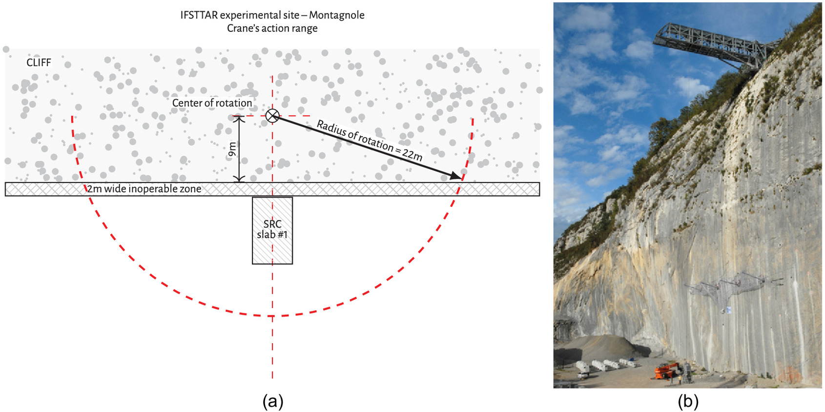
The major equipment of the Gustave Eiffel University experimental rockfall testing station is a tower crane jib installed at the top of a 70-m-high vertical cliff. Loads of up to 200 kN (masses of about 20 t) can be lifted and released using an electrohydraulic hook equipped with a damping device. The maximum impact velocity is about

133 km / h

, and the maximum impact energy is of the order of 13.5 MJ.

Finally, a precast slab, named Slab 1 in Fig. 2(a), is located on the ground level platform. Slab 1 is composed of steel-reinforced concrete (SRC) having 60 cm embedded in the rock substratum. It is 4.5 m wide and 8 m long and was used in this study to simulate a very stiff structure protected by a sand layer that would be impacted by a boulder.

Fig. 2. (a) Schematic plan view; and (b) Gustave Eiffel’s full-scale rockfall experimental testing facility in Montagnole, France. (Image by Bruna Garcia.)

Sand Classification and Protective Soil Layer Construction Procedure

Only one type of granular protective material was considered in this experimental campaign: a rolled and clean alluvial sand. This was done to guarantee that the material remained cohesionless for a long period of time after its placement. Fig. 3 shows the grain size distribution of the clean rolled sand used in this study.

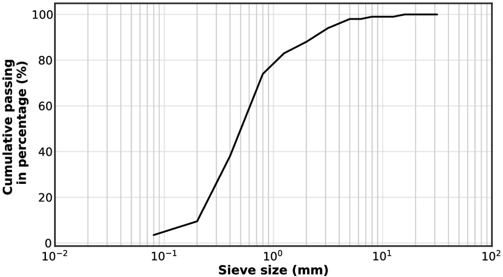
Fig. 3. Grain size distribution of the sand used in the study.

Soil particle sizes ranged from 0 to 4 mm and the fraction passing the 80-μm sieve represents 3.5% in mass. Fig. 4 illustrates the construction of the sand cushion layer over the reinforced concrete slab. As shown in Fig. 4(a), a geotextile was first placed on the slab and surrounding ground surface. The sand cushion layer was placed in successive sublayers, each one 40 cm thick [Fig. 4(b)] and compacted by three passes of a vibrating plate compactor (model MVCF60, Mikasa Shoji, Osaka, Japan) at the maximum traveling speed of about

25 m / \min

, alternating converging and diverging spiral paths [Fig. 4(c)].

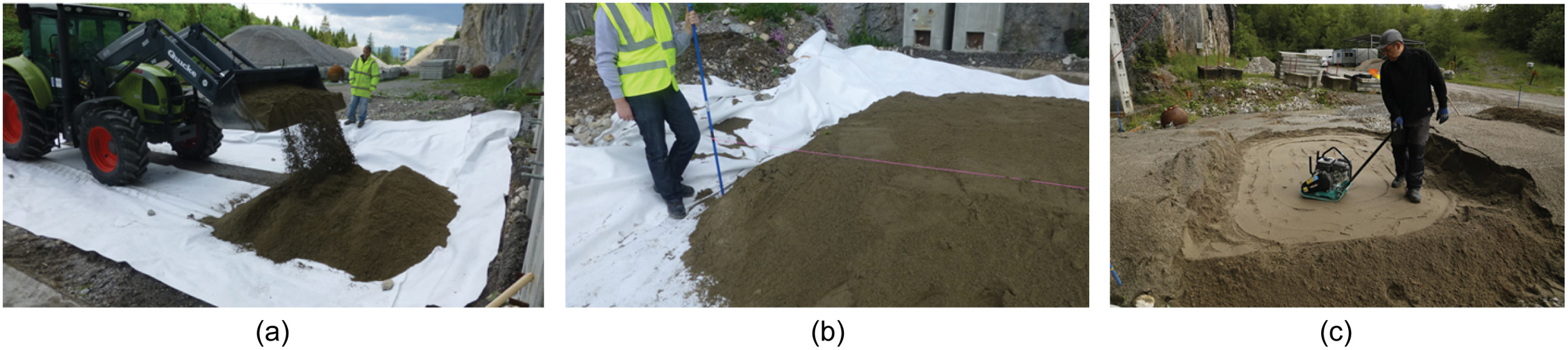
Fig. 4. (a) Soil dumping on geotextile using a backhoe; (b) leveling of the soil sublayers; and (c) soil compaction using a vibrating plate compactor. (Images by Tarik Oussalah.)

The soil’s stiffness presumably has an influence on the pressure transmitted to the protected structure. To reduce the scope of the parametric study to the three impact condition factors

D

,

B

, and

V

, all the tests were performed on the sand cushion layer compacted to the same dry density of about 1.53. After each test, being disturbed by the impact and penetration of the boulder, the sand was removed and the protective sand layer was constructed again, applying the same construction procedure. During construction, the homogeneity of compaction was controlled with in situ PANDA (Sol Solution Company, Riom, France) dynamic penetrometer profiles, and the unit weight of the compacted sand was determined applying the in-place measurement method defined in the NF P 94-061-4 standard (AFNOR 1996).

Instrumentation

Instrumentation included two high-speed cameras (1,000 images per second), a triaxial accelerometer attached to the impacting block, and seven pressure cells installed on the upper surface of the horizontal SRC slab before placing the sand layer. Measurements were synchronized and recorded at an acquisition frequency of 10 kHz.

Fig. 5(a) shows one of the pressure cells used in the experimental tests (Model 3515-1, GEOKON, Lebanon, New Hampshire). Strain gauge sensors are well-suited for the high-frequency data acquisition required in this study. Depending on the cell model type, the measured pressure may range from 0 to 1.5, 3, or 6 MPa, with an accuracy of 0.25% of the full-scale range.

Fig. 5. (a) Granular soil pressure cell; and (b) cells installed in an L-shape on the slab’s upper face. (Images by Tarik Oussalah.)

The seven pressure cells were installed forming an L-shape at the slab’s upper face [Figs. 5(b) and 7]. They were sealed to the slab with quick-setting cement and covered with a plastic film to protect them from water infiltration during the in situ testing period. The right angle of this L, at the center of the slab, was the targeted impact point. The impact test conditions being axisymmetric, the L-shape was devised to check for possible side effects and introduce some redundancy in the data.

Full-Scale Testing Program

Table 1 describes the referencing system used to identify each of the three varied impact conditions factors

D

,

B

, and

V

[related to the free fall height of the boulder (

H

)]. An index from 1 to 5 was used to designate in each test the layer thickness, boulder size, and the impact velocity. For example, Test D2B2H3C2 corresponds to the test where the layer thickness

D

is equal to 1.5 m, the equivalent block diameter

B

is 0.73 m, and the drop height is 10 m (impact velocity

V

of

50.4 km / h

). C2 refers to the layer compaction procedure, the same for all the tests. Fig. 6 shows the five different impacting blocks used in the tests. The first two blocks are spherical, composed of a steel shell filled with concrete.

Table 1. Tests referencing for the different impact condition factor values

Index	Sand cushion layer thickness, $D$ (m)	Boulder diameter, $B$ (m)	Free-fall height, $H$ (m)	Impact speed, $V$ ( $m / s$ )	Impact speed, $V$ ( $km / h$ )
1	1	0.42	1	4.43	16.0
2	1.5	0.73	5	9.90	35.6
3	2	0.73	10	14.00	50.4
4	—	1.54	20	19.81	71.3
5	—	1.78	33	25.45	91.6

Fig. 6. Characteristic dimensions of impacting blocks referenced from 1 to 5.

The three other blocks, with a rhombicuboctahedral shape, are made of steel fiber–reinforced concrete. They were conventionally designed for the full-scale rockfall tests required for the European Certification of Rockfall Protection Kits. Table 2 gives the characteristic properties of each block. In order to represent a similarity to real impacting boulders, the unit mass of all blocks was close to that of most rocks (

2,500 kg / m^{3}

). For the last three impacting blocks,

B

takes the value of the equivalent sphere having exactly the same mass, by assuming an unit mass of

2,500 kg / m^{3}

.

Table 2. Impacting block characteristics and equivalent diameter

B

Block index	Unit mass ( ${kg / m}^{3}$ )	Block mass (kg)	Block diameter, $B$ (m)
1	2,500	117	0.42
2	2,500	553	0.73
3	2,500	543	0.73
4	2,500	4,796	1.54
5	2,500	7,399	1.78

The mass of Block 2, of spherical shape, is close to that of Block 3, of rhombicuboctahedral shape. These two blocks were used to investigate the influence of block shapes on the observed pressure pulse. In the range of protective layer thicknesses and impact velocities considered in this study, no significant influence of the block shape was identified. Thus, as far as transmission of pressure pulse through a sand layer is concerned, blocks with rhombicuboctahedral shape may reasonably be considered as spherical with equivalent diameter

B

for the range of impact condition factors considered in this study (Oussalah 2018, p. 161).

For each of the 35 tests performed in this study, Appendix I presents the impact condition factors

D

,

B

, and

V

according to the referencing convention.

Experimental Setup

Fig. 7 is a schematic representation of the test’s setup and instrumentation plan. A coordinate system was defined, where the origin is at the slab center, the positive

x - axis

is in the direction of the slab’s largest dimension (toward the cliff), the positive

y - axis

is in the direction of the slab’s width, and the

z - axis

is upward vertical. Cross section

{AA}^{'}

includes the three impact test condition factors

D

,

B

, and

H

(the free-fall height, related to impact speed

V

) and their respective sets of values in the experimental program.

Fig. 7. Schematic representation of test setup and instrumentation plan: (a) ${A A}^{'}$ cross section; (b) plan view for pressure cell spacing configuration Config 1; and (c) plan view for pressure cell spacing configuration Config 2.

For all sand cushion layer thicknesses, the extent of the protective fill at the ground level was such that the top surface would be centered on the slab and no less than 7 m long (in the

x

-direction) by 4 m wide (in the

y

-direction) to avoid possible boundary effects when the boulder hits the center of the test’s setup. Axisymmetric mechanical conditions were checked, comparing the pressure measurements on the slab in both

x -

and

y

-direction s.

In Figs. 7(b and c), the two plan views refer to the two configurations of the seven pressure cells locations (in red in the figure, numbered 11 to 17) that were used in the experimental program, called Config1 and Config2 in the figure. In Fig. 7(b) and for Config1, the spacing between the centers of two adjacent pressure cells (of diameter 23 cm) was the same in both the

x -

and

y

-directions, equal to 25 cm. In Config2 [Fig. 7(c)], the spacing between the centers of two adjacent pressure cells was 40 cm in the direction of the fill length (

x

-direction), and 50 cm in the direction of the fill width (

y

-direction).

The first configuration was used for the tests with the smallest cushion layer thickness (

D = 1 m

), and the second was used for the two larger thicknesses (1.5 or 2 m), to account for possible wider diffusion of the forces as the thickness of the sand cushion increases. The pressure cells were placed along two directions from the center of the slab to provide some redundancy in the measurements and to check the assumption of axisymmetric loading conditions. Finally, two high-speed cameras (C#1 and C#2 in the figure) were installed in two horizontal directions.

Data Reduction

Corresponding to a vertical impact on a horizontal homogeneous fill protecting a concrete slab, the impact test conditions were presumably axisymmetric. The pressure measurements at the top of the slab were therefore analyzed in terms of time (

t

) and horizontal (radial) distance (

r

), at the slab surface, from the vertical impact trajectory to the centers of the different pressure cells.

The block was lifted from the targeted impact point at the top surface of the fill, located just above the P17 pressure cell at the right angle of the L-shaped pressure cells setup. In fact, it turned out that due to the electrohydraulic hook dropping mechanism, during the test, the actual impact point observed on the high-speed video recordings might be a few centimeters away from the targeted impact point. In addition, although test conditions were axisymmetric by principle, a slight deviation of the boulder (a few more centimeters in the horizontal direction over the penetration depth) was systematically observed during its penetration in the sand fill.

As a consequence, for the sake of analyzing the results from a series of tests that basically were axisymmetric, the location of the vertical impact trajectory was deemed to be defined by the center of the boulder at the end of the test. For that purpose, the exact position of the block after penetration in the sand fill was determined by triangulation using measured distances from the top of the block to two referenced points sealed in the cliff. Appendix I includes the values of these two impact coordinates, denoted

X_{impact}

and

Y_{impact}

.

Fig. 8 is a schematic representation of a test configuration after impact. As explained previously, in the plan view, the location of the free-fall impact trajectory is defined by the center of the boulder after penetration. In the horizontal plane at the slab level, the radial distances of the pressure cells numbered

P_{1 i}

,

i = 1

to 7, were denoted

r_{(P_{1 i})}

. The beginning of an impact was considered to be the moment when the block immediately touches the protective layer. This location of the block, at the top of the layer on the vertical impact trajectory, defines the initial distance

R_{(P_{1 i})}

,

i = 1

to 7, between the boulder and the pressure cells when the impact begins. This initial distance is related to the horizontal distances between the vertical impact trajectory and pressure cells by Eq. (1)

R_{(P_{1 i})} = \sqrt{D^{2} + {(r_{(P_{1 i})})}^{2}}

(1)

where

D

= protective layer thickness.

Fig. 8. Schematic representation of distances from impact trajectory to the pressure cells.

Results

Fig. 9 illustrates typical induced pressure versus time curves observed at the top of the SRC slab during an impact test. The term induced pressure designates the increment of pressure through the sand layer caused by the impact at the top of the layer, i.e., the total pressure observed in the pressure cells minus the sand layer’s self-weight, a constant value that was observed in the pressure cells before performing the tests. This way, the value of induced pressure is initially equal to zero and, after a certain duration, it returns to zero again.

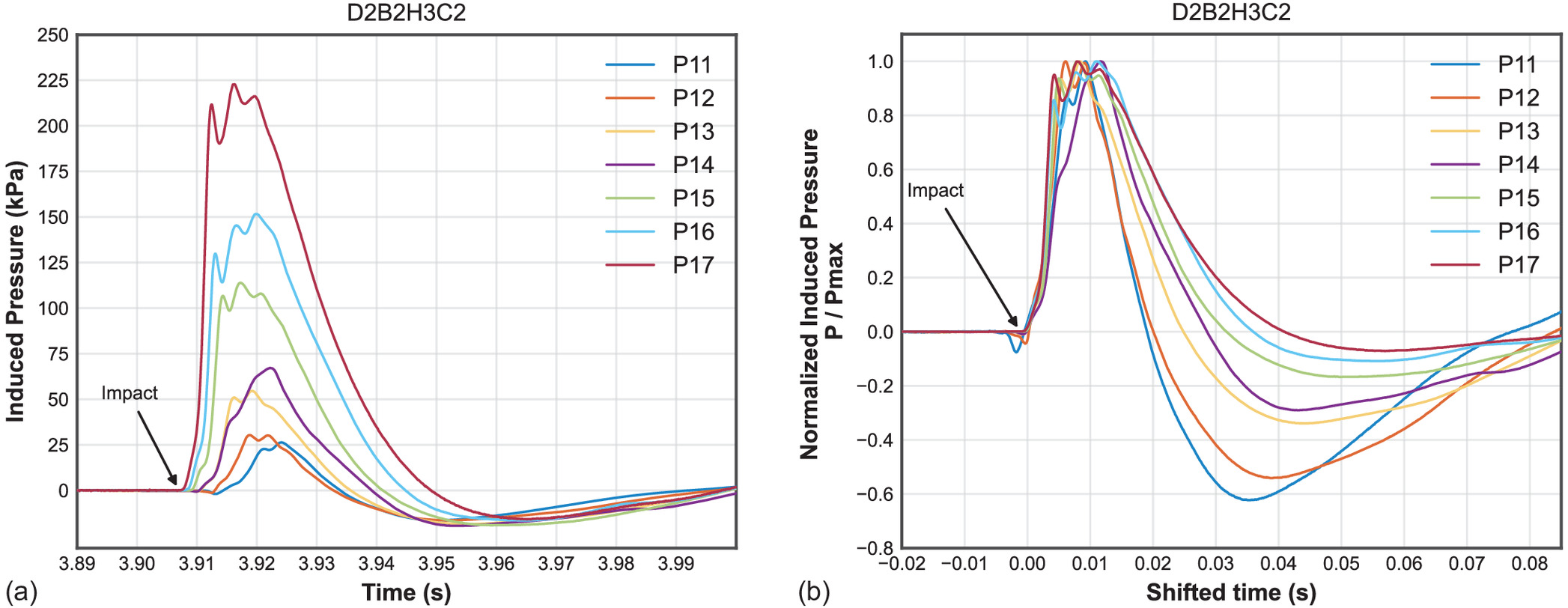
Fig. 9. Analysis of pressure cell measurements in Test D2B2H3C2: (a) induced pressure versus time curves; and (b) normalized induced pressure versus shifted time.

As mentioned in the preceding section, there was an offset between the targeted point at the surface of the sand layer (located above Pressure cell P17) and the final position of the block. In this test (D2B2H3C2), the offset, presented in a plan view in a subsequent figure, was such that P17 was the pressure cell closest to the impact trajectory, leading to the maximum observed value of peak induced pressure in Fig. 9(a). P15 and P16 (Fig. 7 shows the pressure cell numbering in the experimental setup) were located at about the same distance from the trajectory, some 50 cm farther, thus being subjected to similar but lower values of peak induced pressure.

The typical results from Fig. 9(a) illustrate four aspects of the observed behavior, which will help to explain the data reduction procedure presented in the following. First, the moment where the pressure begins to rise in a pressure cell increased within the distance of the cell to the impact trajectory (in the figure, the lower the peak, the larger the distance). Second, the rate at which the pressure rises was lower for the more distant sensors. Third, in the graphs, local oscillations may be noted in the pressure measurements for all the cells. These local high-frequency variations on the curves, of a few milliseconds period duration, were attributed to the natural vibration frequency of the pressure cells, which are protected from punching by two thick steel disks of 23 cm diameter (the first mode natural vibration frequency of a square steel plate of 20 cm length and 2.5 cm thickness is about 500 Hz, i.e., 2 ms duration).

Fourth, after a certain duration, the induced pressure may become negative before returning progressively to zero. In the D2B2H3C2 test, the sand layer thickness was 1.5 m. The self-weight of the layer was of the order of 25 kPa. Therefore, the pressure applied at the top of the slab decreased due to the cushion layer’s self-weight but remained positive (in compression). This phenomenon was related to the dynamic deflection of the slab, delayed by about 30 ms due to its inertia. In all the tests, the pressure remained positive at the sand–slab interface, and no effect of possible subsequent vibration of the slab was observed.

Based on a large amount of cell pressure measurements, the purpose of the data reduction procedure detailed in the following is to represent, for each impact test, the space and time-induced pressure pulse distribution using as few characteristic properties as possible. First, the data reduction procedure to represent the spatial distribution at the slab’s surface of the induced pressure peak values is presented. Secondly, the representation of the induced pressure versus time at a specific distance from the impact trajectory is considered.

Spatial Distribution of Induced Pressure Peak Values at the Slab’s Surface

The peak of induced pressure at different distances from the impact trajectory is a key aspect to describe the time-space-induced pressure pulse transmitted to the slab through the protective sand layer. As shown in Fig. 9(a) for Test D2B2H3C2, a maximum value of induced pressure may be observed during the impact for each pressure cell. In Fig. 10(a), the maximum values of induced pressure at the seven pressure cells (P11 to P17) is plotted as a function of the distance from the center of the pressure cell to the impact trajectory (

r_{P 1 i}

).

Fig. 10. (a) Induced peak pressure as a function of distance from impact point; and (b) impact point on $X Y - plane$ (Test 14, D2B2H3C2).

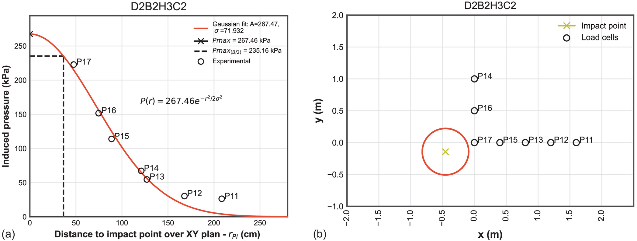
For Test D2B2H3C2, Fig. 10(b) shows the locations of the impact point and of the pressure cells setup in the

X Y - plane

, at the top of the slab. The distribution of induced pressure peak values had to be extrapolated toward the impact trajectory at a distance

r = 0

, as shown in Fig. 10(a). The large number of tests (35) was helpful to develop a good understanding of the shape of the induced pressure peak distribution about the impact trajectory. An axisymmetric distribution was confirmed by the measurements observed along the two lines of pressure cells, in the

x -

and

y

-direction s, which gave close values for cells at similar radial distances to the impact trajectory (

r

). The bell shape of the observed peak values of induced pressure with the distance to the impact trajectory suggested this spatial distribution can be represented using a normal distribution function described by Eq. (2)

P_{\max} (r) = P_{\max x} \cdot e^{- β r^{2}}

(2)

In the data reduction procedure applied to each test, the two parameters in Eq. (2) (

P_{\max x}

and

β

) were determined by nonlinear least-squares fit (Levenberg 1944; Marquardt 1963). Physically, the

P_{\max x}

parameter in fact is the overall maximum value of induced pressure, occurring at

r = 0

, on the impact trajectory. The

β

parameter describes the decay of induced pressure peak values with increasing distance to the impact trajectory. Bearing in mind that the induced pressure spatial distribution might be related to the block size (thus the equivalent diameter

B

), it was decided to consider the peak value of induced pressure at a distance

B / 2

from the impact trajectory, i.e., right below the block’s edge in the direction of impact. The peak value of induced pressure below block’s edge is thus expressed by Eq. (3)

P (B / 2) = P_{\max x} \cdot e^{- β \cdot {(B / 2)}^{2}}

(3)

Conversely, the normal distribution decay of induced pressure peak values with the distance to the impact trajectory (

β

) is related to the induced pressure peak value at the periphery of the block throughout the following Eq. (4):

β = \frac{\ln (P_{\max x} / P_{\max} (B / 2))}{{(B / 2)}^{2}}

(4)

In summary, the spatial distribution of peak values of induced pressure at the surface of the slab during the impact may be represented by Eq. (2). This equation is based on two physical characteristic properties of the induced pressure pulse,

P_{\max x}

and

β

. The first one is the overall peak value of induced pressure on the impact trajectory. The second one characterizes the decay of induced pressure peak values with increasing distance to the impact trajectory. This property was related to the decay of induced pressure peak values from the center to the periphery of the block in the direction of impact.

Time Distribution of the Induced Pressure Pulse

At a given distance from the impact trajectory, the induced pressure at the slab’s surface during an impact on the protective soil layer starts to rise at a specific moment, then rapidly increases to a peak value and finally progressively returns to zero. In the following three subsections, the tests results are analyzed regarding these three aspects. The purpose is still to identify characteristic properties that may be used to represent the time-space-induced pressure pulse transmitted to the slab.

Pressure Pulse Delay at the Sand–Slab Surface

Concerning the pressure pulse at the top of the slab during an impact, as illustrated in Fig. 9(a), showing the induced pressure observed with the pressure cells, the time of impact does not coincide with the moment when the pressure begins to rise in the pressure cells. As a matter of fact, a delay was observed between the moment of impact and when the pressure began to rise in the pressure cell. This delay increased with the distance of the pressure cell to the impact trajectory.

As a consequence, the signal from each pressure cell at the beginning of impact was treated to evaluate the exact moment when the pressure begins to increase, becoming larger than the constant unit weight of the soil layer measured before impact. At each cell, the beginning of the pressure pulse was defined as the moment when the measured pressure exceeds the constant initial pressure by 2.5 times the noise of the recorded signal from the pressure cell before impact. In terms of induced pressure, which was equal to zero before the impact, this moment is when the induced pressure becomes larger than 2.5 the noise in the signal from the pressure cell before impact.

By reference to the propagation of mechanical waves in an elastic media, in Fig. 11, the moment when pressure begins to rise in the pressure cell

P_{(1 i)}

,

i = 1

to 7 (Fig. 8), is plotted versus the distance of the pressure cell to the impact point at the top of the layer, denoted

R (P_{(1 i)})

in Fig. 8. Fig. 11 shows that the time at which the pressure pulse begins at a pressure cell increased linearly with the distance of the pressure cell to the impact point at the top of the layer.

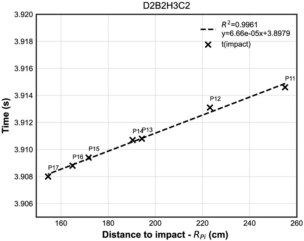
Fig. 11. Time when induced pressure pulse begins versus distance to the impact point at the top of the protective soil layer (Test D2B2H3C2).

The slope of this relationship may be interpreted as the stress propagation velocity through the sand layer. This velocity is denoted as

A_{i}

. An important result from this study is that in all the 35 tests, the same value of the

A_{i}

velocity was found, no matter the layer thickness, block size, or impact speed. For the sand compacted in all the tests to the same density (1.53), this velocity was of the order of

150 m / s

. Such a value is way below the usual velocity of compression wave (

V_{p}

) from seismic refraction geophysical tests in fine dry sands, which varies from 300 to

700 m / s

for loose to dense sands.

In fact, the loading conditions in the sand during impact, producing plastic flow and large strains and displacements, are such that the elastic behavior assumption does not apply. However, this physical phenomenon, characterized by a constant value of the

A_{i}

velocity, independent of the impact factors

D

,

B

, and

V

, is useful information to represent the space-time pressure pulse at the surface of the slab during a rockfall impact. The time at which the pressure on the protected slab begins to increase at a distance

r

from the impact trajectory at the soil–slab interface may be expressed by Eq. (5)

t_{i} (r) = t_{i} (0) + \frac{\sqrt{D^{2} + r^{2}} - D}{A_{i}}

(5)

where

t_{i}

(0) = initial moment, when the pressure at the point on the slab surface corresponding to the impact trajectory (

r = 0

and

R = D

) begins to increase. During the tests, the pressure cells measurements were recorded in function of time. The moment corresponding to

t_{i}

(0) may be defined in Fig. 11 by extrapolating the linear relationship back toward

R = D

, i.e.,

r = 0

. This moment may be used to define a new time origin, meaning that

t_{i} (0) = 0

. With this convention, for the origin of time, the pressure pulse induced by the impact would begin in

r = 0 cm

and at time

t = 0 s

.

Induced Pressure Increase Rate

The moment at which the induced pressure reaches its peak value at a pressure cell location at a distance

r

from the impact trajectory is an important information to describe the pressure pulse caused by the impact. In fact, it governs the loading rate, which is fundamental in dynamic structural design. Unfortunately, as illustrated in Fig. 9(a), presenting the induced pressure observed during impact in the seven pressure cells for Test D2B2H3C2, the moment at which the pressure pulse reached the peak value at a pressure cell location cannot be accurately determined due to local oscillations. In an attempt to estimate whether the time to peak pressure depends on the distance to the impact trajectory, it was decided to plot the normalized induced pressure, i.e., the induced pressure divided by its maximum value during the impact.

In addition, to properly compare the pressure increase duration at each pressure cell, for each normalized induced pressure curve, the value of time was shifted by

t_{i}

(

r

), the delay between the impact time and the moment where the pressure begins to rise at the pressure cell. For Test D2B2H3C2, Fig. 9 shows (1) the observed induced pressure versus time at the different pressure cell locations, and (2) the corresponding normalized induced pressure versus time shifted by

t_{i}

(

r

). The larger negative values of normalized induced pressure, up to

- 0.6

at the P11 pressure cell, correspond to the farthest pressure cells, where the peak values of induced pressure are the lowest, of the order of the unit weight of the protective fill.

As explained previously, the negative values of induced pressure are related to the dynamic deflection of the thick SRC slab. From Fig. 9, it clearly appears that during pressure increase, the normalized induced pressure versus shifted time curves overlap. The same physical phenomenon was systematically observed in all the 35 tests: the rate of increase of normalized induced pressure is therefore independent to the distance to the impact trajectory (

r

). This important physical phenomenon means that the expression for the pressure on the slab induced by an impact is of the general following form described by the following Eqs. (6)–(8):

For

t \leq t_{i} (r)

P (r, t) = 0

(6)

For

t_{i} (r) \leq t < t_{\max} (r)

P (r, t) = P_{\max} (r) \cdot f (t - t_{i} (r))

(7)

and for

t \geq t_{\max} (r)

P (r, t) = P_{\max} (r) \cdot g (r, t - t_{\max})

(8)

where

t_{\max} (r)

= time where the induced pressure reaches its maximum value at a distance

r

from the impact trajectory.

P_{\max} (r)

, the maximum value of induced pressure at a distance

r

from the impact trajectory, was expressed in Eq. (2) in terms of two characteristic properties of the pulse of induced pressure,

P_{\max x}

(the overall maximum induced pressure on the impact trajectory) and

β

(defining the normal distribution of induced pressure peak values with distance to the impact trajectory). Whereas the induced pressure increases to its peak value [Eq. (7)], the normalized induced pressure is only a function of time [function

f

in Eq. (7)]. However, although the pressure decreases, the normalized induced pressure is a function of both time and distance to the impact trajectory [function

g

in Eq. (8)].

Unfortunately, it may also be pointed out from Fig. 9 that due to the local oscillations in the pressure cells’ measurements, such a representation of the test’s results does not help to determine the time at which the peak of pressure occurs at the different pressure cell locations. As a consequence, to represent the induced pressure pulse prior to its peak value at a distance

r

from the impact trajectory [i.e., to define the

f

function in Eq. (7)], the most reliable approach was to consider the time-rate increase of normalized induced pressure, which is the same at any point on the slab. In each test, only a few pressure cells’ measurements were affected by local oscillations during pressure increase, like P14 in Test D2B2H3C2 (Fig. 9). In the data reduction process, the measurements from these pressure cells produced results that were obviously inconsistent with others.

The time-rate increase of normalized induced pressure prior to peak value was therefore assumed to be characterized by the slope of the normalized induced pressure versus shifted time curve at 50% of the peak value, denoted

p_{50}

. As may be noticed in Fig. 12, the value of this slope

p_{50}

, away from the start of the curve at

t - t_{i}

and from the oscillations near the peak, is a reliable characteristic property of all the curves. It is a representative property of the rate of loading on the protected slab during the impact.

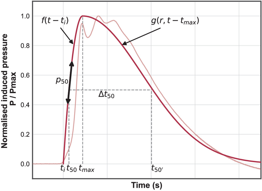
Fig. 12. Normalized induced pressure versus time.

In Fig. 9(b), the shape of the curves prior to peak led to represent the normalized induced pressure versus shifted time (the

f

function) with a parabolic relationship based on three properties of the curves: (1) its value is zero at time

t_{i}

, (2) the slope is

p_{50}

when the value is 0.5, and (3) the slope is zero at the top, where the value is one (at the peak). Such a parabolic

f

function is represented in Fig. 12. The parabolic function representing the relationship between normalized induced pressure versus time before peak pressure is given by the following Eq. (9):

f (t - t_{i} (r)) = - \frac{{(p_{50})}^{2}}{2} \cdot {(t - t_{i} (r))}^{2} + \sqrt{2} \cdot (p_{50}) \cdot (t - t_{i} (r))

(9)

For each impact test, the characteristic property

p_{50}

was obtained from the data reduction procedure applied to the pressure cells measurements. The value of

t_{i}

(

r

), the time at which the pressure starts to increase at a distance

r

from the impact trajectory on the slab, was given by Eq. (5).

The previous equation may be used to calculate the time

t_{\max}

at which the induced pressure reaches its maximum at a distance

r

from the impact trajectory as follows:

t_{\max} (r) = \frac{\sqrt{2}}{p_{50} (r)} + t_{i} (r)

(10)

Similarly, the time

t_{50}

at which 50% of the maximum induced pressure occurs (corresponding to the point where the slope

p_{50}

is determined), is given by the following:

t_{50} (r) = \frac{\sqrt{2} - 1}{p_{50}} + t_{i} (r)

(11)

Pulse Duration and Induced Pressure Unloading Rate

To complete the description of the pressure pulse at a distance

r

from the impact trajectory, the decrease of normalized induced pressure versus time after the peak, i.e., the

g

function in Eq. (8), has to be characterized. In fact, for dynamic structural design, the unloading rate is as important as the loading rate. Considering the pressure measurements, defining the duration of unloading after the peak of pressure did not appear to be the most effective approach to characterize the unloading rate because the induced pressure rapidly drops after the peak and very progressively returns to zero [Fig. 9(a)]. Besides, the dynamic behavior of the slab impaired the measurements for the larger times after impact (larger than about 30 ms after impact).

In addition, as explained previously, the local oscillations in the pressure measurements did not allow precise identification of the time at which the induced pressure reached its maximum at a distance

r

from the impact trajectory [

t_{\max}

(

r

)]. Therefore, the most effective approach to evaluate the unloading rate appeared to be relying on the time during which the pressure is greater than 50% of its peak value (or normalized induced pressure greater than 0.5). This duration, represented in Fig. 12, is denoted

Δ t_{50}

. The local oscillations in the measurements when pressure is initially rising and after the peak decreasing may introduce some uncertainties in the determination of

Δ t_{50}

for some of the pressure cells. However, this data reduction process turned out to produce consistent and reliable values of

Δ t_{50}

.

As illustrated by Fig. 9(b), the duration of the normalized induced pressure pulse depended on the distance to the impact trajectory. The closer to the impact trajectory (Pressure cell P17), the longer the pulse duration. To investigate this relationship, the values of

Δ t_{50}

from the seven pressure cells were plotted versus the distance to the impact trajectory (

r

). Fig. 13 shows this graph for Test D2B2H3C2. Such a linear relationship was consistently observed in all 35 impact tests. Thus the value of

Δ t_{50}

at a distance

r

from the impact trajectory may be expressed as follows:

Δ t_{50} = Δ t_{50} (r = 0) - \frac{r}{A_{50}}

(12)

where

Δ t_{50}

(0) = time during which the induced pressure on the impact trajectory remains larger than 50% of its peak value; and

A_{50}

= inverse value of the slope of the linear relationship of the graph in Fig. 13. It has the dimension of a velocity.

Fig. 13. Time duration on which the pressure is greater than 50% of peak value in the pressure cells at different distances to the impact trajectory (Test D2B2H3C2).

For each impact test, the

y - intercept

Δ t_{50}

(0) and the slope inverse

A_{50}

are two characteristic properties of the space-time pressure pulse transmitted to the structure during the impact on the protective soil layer. The results of the linear regression at the top of the graph in Fig. 13 indicate that for Test D2B2H3C2,

Δ t_{50}

(0) was 21.74 ms, and

A_{50}

was about

165 m / s

.

The shape of the normalized induced pressure curve after the peak and its progressive decrease to zero suggest to consider for the

g

function a Gaussian function, centered at the peak, where

t = t_{\max}

. At this point, the derivatives of both expressions for the pressure pulse before the peak (function

f

) and after the peak (function

g

), are zero. Consequently, the

g

function is given the following form. For

t \geq t_{\max}

(

r

), it is

g_{(r, t)} = e^{- γ_{(r)} \cdot {(t - t_{\max} (r))}^{2}}

(13)

where

γ

(

r

) = normalized induced pressure decay rate beyond the peak, which depends on the distance

r

to the impact trajectory.

At a distance

r

from the impact trajectory, the decay of normalized induced pressure beyond the peak [

γ (r)

] is in fact related to the duration of the pressure pulse, which may be represented by the duration

Δ t_{50}

(

r

). Given that the

g

function in Eq. (13) equals

1 / 2

when time is equal to

t_{50}

(

r

) plus

Δ t_{50}

(

r

), and substituting

t_{\max}

(

r

) by its expression in Eq. (10) and

t_{50}

(

r

) in Eq. (11), the following expression for

γ

(

r

) may be derived:

γ_{(r)} = \frac{\ln (2) \cdot p_{50}^{2}}{{(p_{50} \cdot Δ t_{50} (r) - 1)}^{2}}

(14)

where

p_{50}

= rate of increase of the normalized induced pressure before peak, as defined previously;

Δ t_{50}

(

r

) = duration of the pressure pulse above 50% of its maximum, given by Eq. (12); and

p_{50}

= characteristic property of the induced pressure pulse, as well as

Δ t_{50}

(0) and

A_{50}

in Eq. (12).

Conclusion

A total of 35 instrumented tests were performed with a sand layer up to 2 m thick, rock boulder size up to 1.78 m (mass 7,399 kg), and impact velocity up to

91 km / h

. The sand layer construction procedure was the same for all the tests, and the sand’s dry density was 1.53. The pressure transmitted through the protective sand layer during the impact was observed using pressure cells located on the structure at several distances from the impact trajectory. The analysis of tests results allowed observation of several physical phenomena, which were then employed to identify characteristic properties defining the space-time pressure pulse at the surface of the structure induced by the impact on the sand layer.

Physical phenomena may be observed. First, the time at which the pressure induced by the impact at the surface of the structure began to rise, denoted

t_{i}

(

r

), increased linearly with the distance to the impact point at the top of the protective layer (

R

), defining an initial propagation velocity of the induced pressure. The same value of initial propagation velocity (

A_{i}

) was observed in all the tests. This characteristic property was thus found to be independent of

D

,

B

, and

V

. It may, however, pertain to the sand’s grain size distribution and dry density, which were constant in all tests.

Second, the time-rate increase of the normalized induced pressure (the pressure divided by its maximum value during impact) was observed to be independent of the distance to the impact trajectory. This physical phenomenon implies that during pressure increase, the space and time variables may be separated in the expression for

p (r, t)

, as represented by Eq. (7).

The maximum induced pressure value [

P_{\max} (r)

] was represented by a Gaussian distribution centered on the impact trajectory (

r = 0

). The distribution was then defined by the two following characteristic properties: the maximum induced pressure on the impact trajectory (

P_{\max x}

) and the decay rate

β

, which was related the maximum induced pressure value observed at the block’s periphery:

P_{\max} (r = B / 2)

.

Two functions,

f

and

g

, were defined to represent the normalized induced pressure as function of time, respectively during pressure increase and decrease. The function

f

does not depend on the distance to the impact trajectory. These two functions were defined using three additional characteristic properties of the normalized induced pressure pulse:

•

p_{50}

, which is the time-rate of increase of normalized induced pressure when the pressure reaches 50% of its peak value, which was found to be independent of

r

.

•

Δ t_{50}

(0), which is the duration of time where the induced pressure on the impact trajectory remains larger than 50% of its peak value.

•

A_{50}

, which is the velocity that describes the linear decrease of

Δ t_{50}

(

r

) with the distance to the impact trajectory (

r

). In other words, the decrease of the duration of the normalized induced pressure pulse with the distance to impact trajectory. This velocity was related to the value

Δ t_{50}

(

B / 2

).

The values of the five characteristic properties of the induced pressure pulse [

P_{\max x}

,

β

,

p_{50}

,

Δ t_{50}

(0), and

A_{50}

] for the 35 impact tests have been gathered in Appendix II. For each impact test condition

D

,

B

, and

V

, the induced pressure pulse at the slab surface during the impact may be represented using the expressions for

P_{\max}

(

r

),

f

, and

g

and computed with the corresponding characteristic properties in Appendix II. In practice, considering a rockfall hazard defined as a block of equivalent diameter

B

and impact velocity

V

, and assuming a protective sand layer of thickness

D

, an approximate induced space-time pressure pulse distribution

p (r, t)

at the surface of the protected structure may already be estimated selecting the appropriate properties values in Appendix II. The structure subjected to such a space-time pressure pulse may then be designed in dynamic conditions as explained for example by Kappos (2002).

It may be assumed that the approach presented in this study to define the space-time pressure pulse distribution overestimates the actual pressure pulse for two reasons. First, the tests were performed on a very stiff structure (a concrete slab 60 cm thick cast in place on a rock substratum). Should a more flexible structure be considered, lower induced pressure values would have been observed. Second, in this study, the impact was perpendicular to the protected structure. For a lower impact angle, the induced pressure values would probably be lower because a larger mass of the soil layer would be displaced. However, it must be emphasized that this approach does not apply for any block shape. For an elongated block shape, the impact on a sharp edge or the smallest side will lead to deeper penetration, larger peak, and narrower spatial distribution of induced pressure.

Notation

The following symbols are used in this paper:

$B$: block’s diameter (m);
$D$: sand cushion layer thickness (m);
$d$: block’s characteristic dimension (m);
$H$: release height (m);
$V$: impact speed ( $m / s$ ); and
$w$: steel-reinforced concrete slab thickness (m).

Appendix I. Experimental Tests Referencing for Given Impact Coordinates ( $x$ and $y$ )

Test	$D$	$B$	$H$	$X_{impact}$ (cm)	$Y_{impact}$ (cm)
1	1	1	1	$- 16.22$	5.92
2	1	1	2	$- 42.01$	27.50
3	1	1	3	$- 52.31$	$- 9.99$
4	1	1	4	$- 68.52$	$- 9.51$
5	1	2	1	$- 6.45$	$- 3.30$
6	1	2	2	$- 10.96$	0.57
7	1	2	3	$- 11.49$	3.59
8	1	2	4	$- 19.89$	8.46
9	2	1	1	$- 25.27$	$- 12.20$
10	2	1	2	$- 23.43$	$- 13.47$
11	2	1	3	$- 43.14$	$- 17.05$
12	2	1	4	$- 32.77$	$- 15.16$
13	2	2	1	$- 25.17$	$- 18.58$
14	2	2	2	$- 45.58$	$- 5.99$
15	2	2	3	$- 45.78$	$- 14.23$
16	2	2	4	$- 45.78$	$- 14.23$
17	2	4	1	$- 22.99$	18.05
18	2	4	2	$- 44.52$	0.70
19	2	4	3	$- 16.70$	$- 9.10$
20	2	4	4	$- 12.52$	$- 2.14$
21	2	5	1	$- 69.94$	0.17
22	2	5	2	$- 44.01$	20.14
23	2	5	3	$- 32.07$	$- 3.78$
24	2	5	4	$- 24.92$	$- 42.87$
25	1	4	1	$- 21.23$	20.72
26	3	5	4	$- 10.87$	$- 4.04$
27	3	5	3	$- 19.50$	16.83
28	3	1	1	$- 34.97$	6.75
29	3	1	2	$- 33.88$	23.05
30	3	1	3	$- 42.70$	15.51
31	3	1	4	$- 38.80$	59.41
32	3	2	1	$- 23.63$	0.33
33	3	2	2	$- 20.68$	$- 13.69$
34	3	4	5	$- 25.76$	0.01
35	3	3	3	$- 7.92$	12.08

Appendix II. Characteristic Properties of the Space-Time-Induced Pressure Pulse Distribution for the 35 Tests

Test	$D$ (cm)	$B$ (m)	$B / D$	$H$ (m)	Impact speed ( $m / s$ )	Impact speed ( $km / h$ )	$P_{\max x}$ (kPa)	$β$	$p 50$ ( $s^{- 1}$ )	$Δ t_{50} (0)$ (ms)	$A_{50}$ ( $m / s$ )	$P_{(B / 2)}$ (kPa)	$Δ t_{50} (B / 2)$ (ms)
1	100	0.42	0.42	1	4.43	15.95	22.09	$1.15 \times 10^{- 4}$	729.29	23.80	46.87	21.00	19.30
2	100	0.42	0.42	5	9.90	35.66	48.37	$1.52 \times 10^{- 4}$	804.31	29.30	58.86	45.23	25.70
3	100	0.42	0.42	10	14.01	50.43	74.32	$1.31 \times 10^{- 4}$	253.76	17.90	184.64	70.13	16.80
4	100	0.42	0.42	20	19.81	71.31	176.36	$1.16 \times 10^{- 4}$	671.37	10.20	1,130.59	167.58	10.00
5	100	0.73	0.73	1	4.43	15.95	77.81	$2.62 \times 10^{- 4}$	95.12	37.40	76.83	54.89	32.60
6	100	0.73	0.73	5	9.90	35.66	217.17	$1.97 \times 10^{- 4}$	480.34	27.90	91.72	166.93	23.90
7	100	0.73	0.73	10	14.01	50.43	348.49	$2.05 \times 10^{- 4}$	455.38	22.80	83.87	265.19	18.40
8	100	0.73	0.73	20	19.81	71.31	705.07	$1.96 \times 10^{- 4}$	741.09	21.30	83.23	542.91	16.90
9	150	0.42	0.28	1	4.43	15.95	8.51	$7.04 \times 10^{- 5}$	541.78	23.20	146.15	8.25	21.80
10	150	0.42	0.28	5	9.90	35.66	32.28	$5.86 \times 10^{- 5}$	752.03	20.40	119.68	31.46	18.60
11	150	0.42	0.28	10	14.01	50.43	46.79	$5.12 \times 10^{- 5}$	284.74	19.30	162.84	45.75	18.00
12	150	0.42	0.28	20	19.81	71.31	82.86	$6.55 \times 10^{- 5}$	274.45	13.40	318.87	80.50	12.70
13	150	0.73	0.49	1	4.43	15.95	39.76	$1.06 \times 10^{- 4}$	570.87	38.90	69.11	34.52	33.60
14	150	0.73	0.49	5	9.90	35.66	104.26	$7.98 \times 10^{- 5}$	364.88	30.70	97.50	93.74	26.90
15	150	0.73	0.49	10	14.01	50.43	267.47	$9.66 \times 10^{- 5}$	320.71	21.70	160.79	235.16	19.50
16	150	0.73	0.49	20	19.81	71.31	341.45	$7.70 \times 10^{- 5}$	574.15	20.30	153.76	308.17	17.90
17	150	1.58	1.05	1	4.43	15.95	288.61	$1.42 \times 10^{- 4}$	294.51	53.70	40.06	118.97	34.00
18	150	1.58	1.05	5	9.90	35.66	757.12	$1.04 \times 10^{- 4}$	743.89	39.60	111.36	394.95	32.50
19	150	1.58	1.05	10	14.01	50.43	944.76	$1.04 \times 10^{- 4}$	89.63	36.40	112.24	492.34	29.40
20	150	1.58	1.05	20	19.81	71.31	2,127.05	$1.17 \times 10^{- 4}$	149.66	30.40	108.41	1,021.69	23.10
21	150	1.79	1.19	1	4.43	15.95	401.00	$9.24 \times 10^{- 5}$	106.85	58.70	52.39	191.32	41.60
22	150	1.79	1.19	5	9.90	35.66	1,041.78	$1.19 \times 10^{- 4}$	212.84	41.10	109.33	401.03	32.90
23	150	1.79	1.19	10	14.01	50.43	1,203.58	$9.19 \times 10^{- 5}$	170.08	45.00	82.61	576.37	34.20
24	150	1.79	1.19	20	19.81	71.31	3,006.73	$1.11 \times 10^{- 4}$	451.01	39.10	71.35	1,236.87	26.50
25	100	1.58	1.58	1	4.43	15.95	553.83	$2.34 \times 10^{- 4}$	318.49	47.80	47.65	128.81	31.20
26	200	1.79	0.90	20	19.81	71.31	1,259.98	$6.06 \times 10^{- 5}$	370.58	38.40	113.92	775.18	30.60
27	200	1.79	0.90	10	14.01	50.43	968.65	$4.61 \times 10^{- 5}$	362.37	39.20	103.59	669.62	30.60
28	200	0.42	0.21	1	4.43	15.95	8.17	$3.25 \times 10^{- 5}$	558.66	11.90	2,575.99	8.06	12.00
29	200	0.42	0.21	5	9.90	35.66	28.21	$4.11 \times 10^{- 5}$	526.32	15.00	437.80	27.70	14.50
30	200	0.42	0.21	10	14.01	50.43	49.84	$4.60 \times 10^{- 5}$	284.94	14.10	491.81	48.84	13.60
31	200	0.42	0.21	20	19.81	71.31	74.67	$3.75 \times 10^{- 5}$	422.05	12.80	526.68	73.44	12.40
32	200	0.73	0.37	1	4.43	15.95	20.53	$3.75 \times 10^{- 5}$	159.43	39.30	72.11	19.53	34.20
33	200	0.73	0.37	5	9.90	35.66	86.49	$4.89 \times 10^{- 5}$	303.21	20.40	233.79	81.04	18.90
34	200	1.58	0.79	33	25.45	91.60	2,165.61	$6.87 \times 10^{- 5}$	494.10	37.60	84.04	1,410.47	28.20
35	200	0.73	0.37	10	14.01	50.43	641.00	$6.10 \times 10^{- 5}$	140.45	38.00	90.31	590.98	34.00

References

AFNOR (Association Française de Normalisation). 1996. Sols: Reconnaissance et essais—Détermination de la masse volumique d'un matériau en place—Partie 4: méthode pour matériaux grossiers (Dmax > 50 mm). NF P 94-061-4. Paris: AFNOR.

Google Scholar

ASTRA–Swiss Federal Transportation Office. 2008. Actions de chutes de pierres sur les galeries de protection. Berne, Switzerland: Office fédéral des routes.

Google Scholar

Bhatti, A. 2015. “Falling-weight impact response for prototype RC type rock-shed with sand cushion.” Mater. Struct. 48 (10): 3367–3375. https://doi.org/10.1617/s11527-014-0405-5.

Google Scholar

Calvetti, F., and C. Di Prisco. 2012. “Rockfall impacts on sheltering tunnels: Real-scale experiments.” Géotechnique 62 (10): 865–876. https://doi.org/10.1680/geot.9.P.036.

Google Scholar

Calvetti, F., and M. Vecchiotti. 2005. “Experimental and numerical study of rock-fall impacts on granular soils.” Rivista Italiana di Geotecnica 4 (4): 95–109.

Google Scholar

Durville, J. L., P. Guillemin, P. Berthet Rambaud, and D. Subrin. 2010. “Etat de l’art sur le dimensionnement des dispositifs de protection contre les chutes de blocs.” Laboratoire Central des Ponts et Chaussées (LCPC). Accessed April 16, 2022. https://hal.archives-ouvertes.fr/hal-00508901.

Google Scholar

Heidenreich, B. 2004. Small-and half-scale experimental studies of rockfall impacts on sandy slopes. Rep. No. Lausanne, Switzerland: École Polytechnique Fédérale de Lausanne.

Google Scholar

Japan Road Association. 2000. Rockfall countermeasure handbook. [In Japanese.] Tokyo: Japan Road Association.

Google Scholar

Kappos, A. 2002. Dynamic loading and design of structures. London: Spon Press.

Google Scholar

Kishi, N., H. Konno, K. Ikeda, and K. Matsuoka. 2002. “Prototype impact tests on ultimate impact resistance of PC rock-sheds.” Int. J. Impact Eng. 27 (9): 969–985. https://doi.org/10.1016/S0734-743X(02)00019-2.

Google Scholar

Labiouse, V., F. Descoeudres, and S. Montani. 1996. “Experimental study of rock sheds impacted by rock blocks.” Struct. Eng. Int. 6 (3): 171–176. https://doi.org/10.2749/101686696780495536.

Google Scholar

Levenberg, K. 1944. “A method for the solution of certain non-linear problems in least squares.” Q. Appl. Math. 2 (2): 164–168. https://doi.org/10.1090/qam/10666.

Google Scholar

Marquardt, D. W. 1963. “An algorithm for least-squares estimation of nonlinear parameters.” J. Soc. Ind. Appl. Math. 11 (2): 431–441. https://doi.org/10.1137/0111030.

Google Scholar

Montani Stoffel, S. 1998. “Sollicitation dynamique de la couverture des galeries de protection lors de chutes de blocs.” Ph.D. thesis, Laboratoire de Mecanique des Roches, École Polytechnique Fédérale de Lausanne, Switzerland.

Google Scholar

Oussalah, T. 2018. “Comportement des sables sous sollicitation d’impact à faible vitesse: Application au dimensionnement de couches de sol protégeant les structures des impacts rocheux.” Ph.D. thesis, Laboratoire Risques rocheux et ouvrages géotechniques, Université de Lyon.

Google Scholar

Pichler, B., C. Hellmich, and H. Mang. 2005. “Impact of rocks onto gravel design and evaluation of experiments.” Int. J. Impact Eng. 31 (5): 559–578. https://doi.org/10.1016/j.ijimpeng.2004.01.007.

Google Scholar

Schellenberg, K. 2008. “On the design of rockfall protection galleries.” Ph.D. thesis, Institute of Structural Engineering, ETH Zürich.

Google Scholar

Yoshida, H., H. Masuya, and T. Ihara. 1988. “Experimental study of impulsive design load for rock sheds.” In Vol. 3 of Proc., IABSE, 61–74. Zürich, Switzerland: International Association for Bridge and Structural Engineering.

Google Scholar

Information & Authors

Information

Published In

Journal of Geotechnical and Geoenvironmental Engineering

Volume 150 • Issue 4 • April 2024

Copyright

This work is made available under the terms of the Creative Commons Attribution 4.0 International license, https://creativecommons.org/licenses/by/4.0/.

History

Received: Mar 21, 2023

Accepted: Nov 3, 2023

Published online: Feb 7, 2024

Published in print: Apr 1, 2024

Discussion open until: Jul 7, 2024

Authors

Affiliations

Bruna Garcia https://orcid.org/0000-0002-6547-9564 [email protected]

Postdoctoral Researcher, Département Géotechnique, Environnement, Risques naturels et Sciences de la terre (GERS), Laboratoire Risque Rocheux et Ouvrages Géotechniques (RRO), Université Gustave Eiffel, 25 Ave. François Mitterand, Case 24 Cité des mobilités, Bron F-69675, France (corresponding author). ORCID: https://orcid.org/0000-0002-6547-9564. Email: [email protected]

View all articles by this author

Tarik Oussalah [email protected]

Geotechnics and Natural Hazards Specialist, Ministère de la Transition Écologique, Direction Générale de la Prévention des Risques, Pôle National de la Sécurité des Ouvrages Hydrauliques, 17 Boulevard Joseph Vallier, Grenoble 38100, France. Email: [email protected]

View all articles by this author

Jean-Pierre Rajot https://orcid.org/0000-0003-1535-3944 [email protected]

Professor and Assistant Geotechnical Department Manager, Département Géotechnique, Environnement, Risques naturels et Sciences de la terre (GERS), Laboratoire Risque Rocheux et Ouvrages Géotechniques (RRO), Université Gustave Eiffel, 25 Ave. François Mitterand, Case 24 Cité des mobilités, Bron F-69675, France. ORCID: https://orcid.org/0000-0003-1535-3944. Email: [email protected]

View all articles by this author

Anne-Sophie Colas [email protected]

Professor, Research Engineer, Département Géotechnique, Environnement, Risques naturels et Sciences de la terre (GERS), Laboratoire Risque Rocheux et Ouvrages Géotechniques (RRO), Université Gustave Eiffel, 25 Ave. François Mitterand, Case 24 Cité des mobilités, Bron F-69675, France. Email: [email protected]

View all articles by this author

Metrics & Citations

Metrics

Citations

Download citation

If you have the appropriate software installed, you can download article citation data to the citation manager of your choice. Simply select your manager software from the list below and click Download.

Abstract

Introduction

Methodology

Experimental Tests

Experimental Full-Scale Rockfall Testing Facility

Sand Classification and Protective Soil Layer Construction Procedure

Instrumentation

Full-Scale Testing Program

Experimental Setup

Data Reduction

Results

Spatial Distribution of Induced Pressure Peak Values at the Slab’s Surface

Time Distribution of the Induced Pressure Pulse

Pressure Pulse Delay at the Sand–Slab Surface

Induced Pressure Increase Rate

Pulse Duration and Induced Pressure Unloading Rate

Conclusion

Notation

Appendix I. Experimental Tests Referencing for Given Impact Coordinates (x and y)

Appendix II. Characteristic Properties of the Space-Time-Induced Pressure Pulse Distribution for the 35 Tests

References

Information

Published In

Copyright

History

ASCE Technical Topics:

Authors

Affiliations

Metrics

Citations

Download citation

Figures

Other

Share

Copy the content Link

Share with email

Share

Request Username

Create a new account

Change Password

Password Changed Successfully

Verify Phone

Congrats!

Appendix I. Experimental Tests Referencing for Given Impact Coordinates ( $x$ and $y$ )