Calibration of Pore Pressure Model for the Liquefaction Prediction of Soils Based on Behavior of Clean Sand, Magnitude Scaling Factor, and Initial Stress Level

Kim, Hyeong-Joo; Dinoy, Peter Rey; Kim, Hyeong-Soo; Park, Tae-Woong; Jeong, Young-Soung

doi:10.1061/JGGEFK.GTENG-11447

Open access

Technical Papers

May 27, 2023

Calibration of Pore Pressure Model for the Liquefaction Prediction of Soils Based on Behavior of Clean Sand, Magnitude Scaling Factor, and Initial Stress Level

Authors: Hyeong-Joo Kim, Ph.D., M.ASCE [email protected], Peter Rey Dinoy, Ph.D. https://orcid.org/0000-0002-5884-1748 [email protected], Hyeong-Soo Kim, Ph.D. [email protected], Tae-Woong Park, Ph.D. [email protected], and Young-Soung Jeong [email protected]Author Affiliations

Publication: Journal of Geotechnical and Geoenvironmental Engineering

Volume 149, Issue 8

https://doi.org/10.1061/JGGEFK.GTENG-11447

PDF

Abstract

The pore pressure model was developed in the past to predict liquefaction induced by an earthquake. Its main advantage is that its parameters can be obtained from experiments based on direct measurement of pore pressure data. However, two downsides of the pioneering model are that its parameters are distinct for each relative density, and that liquefaction curves derived from the model have not been evaluated fully based on well-known triggering liquefaction curves. This research advances the pore pressure model by introducing a method of adjusting the incremental pore pressure rise using calibration factors. Based on the behavior of clean sand, calibration factors, which take into account the effect of the critical stress ratio, earthquake magnitude, and initial stress level, were derived. The calibrated pore pressure model was compared with data from direct simple shear tests to verify the derived calibration factors, and good agreement between the measured and predicted data was observed.

Introduction

The cyclic liquefaction of saturated soils is a subject of paramount significance because of its widespread engineering implications (Yang et al. 2022), and it has attracted considerable interest from researchers and engineers from both geotechnical and seismic fields (Wei 2021). Pore pressure models can be a valuable tool in understanding the liquefaction mechanism of sand because they can predict pore pressure rise based on direct measurement of pore pressure data, and can determine major factors that affect incremental pore pressure rise. Ishibashi et al. (1977) proposed a simple pore pressure model that predicts the pore pressure rise under uniform and nonuniform dynamic shear stresses based on undrained cyclic shear experiments conducted on loose saturated Ottawa sand. Sherif et al. (1978) then extended the pore pressure model and applied it to predict the pore pressure rise of Ottawa sand at three different densities under earthquakelike loading. However, four of the parameters in the model are unique for each density. In addition, the cyclic resistance ratios (CRRs) that were obtained from the model were not evaluated fully based on field performance data because studies of liquefaction were still in their infancy stage at that time. Calibration by successively tracing pore pressure change was difficult because of the lack of accurate information concerning the characteristics of incremental pore pressure change (Ishihara and Li 1972).

The cyclic resistance ratio versus a magnitude 7.5 earthquake, as defined by Seed and Idriss (1982), is equivalent to the cyclic stress ratio (CSR) that can cause liquefaction of a sample in the laboratory at 15 cycles. Seed et al. (1985) summarized data from Pan-America, Japan, and China, and developed a relationship between the cyclic resistance ratio and standard penetration test (SPT) blow count

(N_{1})_{60}

for clean sand (clay content

\leq 5 %

) under a magnitude 7.5 earthquake. The relationship subsequently was modified by various researchers, including with relationships proposed by Youd et al. (2001) and Idriss and Boulanger (2004) (Fig. 1), and the CRR varied nonlinearly with relative density (

D_{r}

).

Fig. 1. Relationship of CRR and $(N_{1})_{60}$ for clean sand and Ottawa sand under a magnitude ( $M_{w}$ ) 7.5 earthquake.

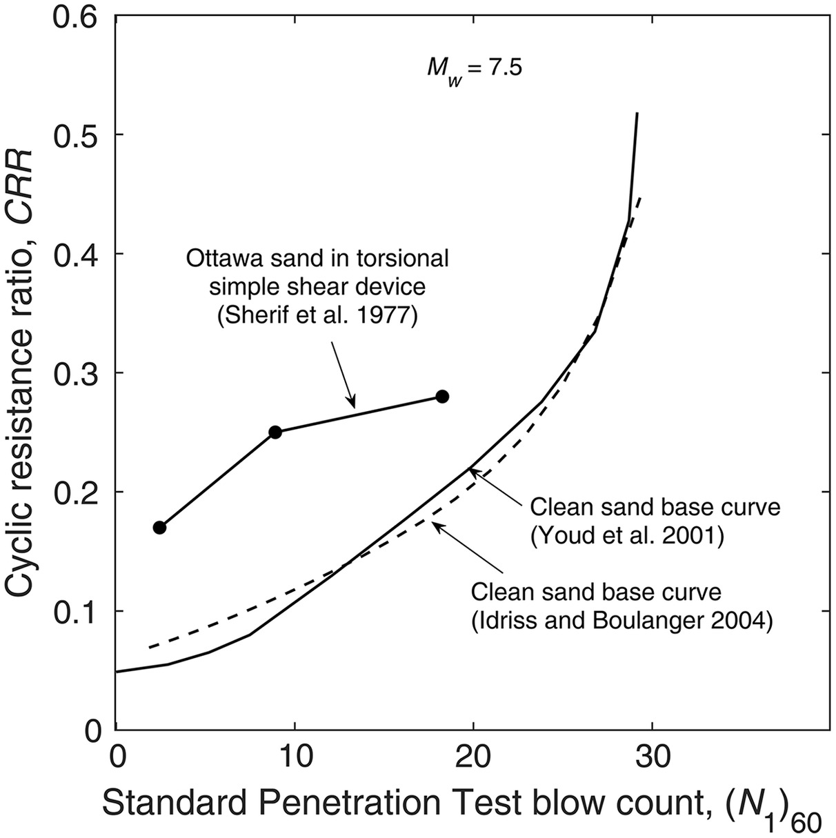
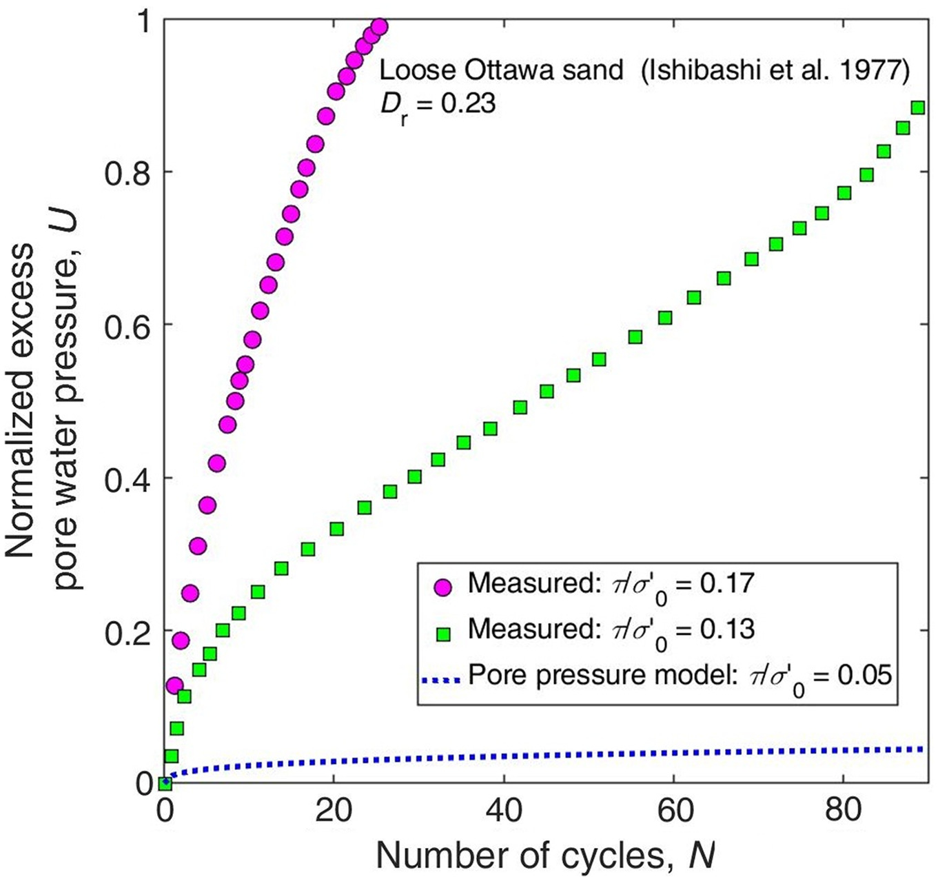
Experiments conducted by Ishibashi et al. (1977) on loose Ottawa sand

(D_{r} = 0.23)

under uniform loading using the torsional simple shear device resulted in the complete liquefaction of the samples after about 25 and 90 cycles when the applied stress ratios were 0.17 and 0.13, respectively (Fig. 2). This study introduces the term “complete liquefaction” to denote the condition in which the excess pore water pressure is equal to or greater than the initial effective stress. Based on the relationship given by Youd et al. (2001) for clean sand (Fig. 1), the CRR for the same relative density would be about 0.05. This means that the samples in Fig. 2 should have liquefied completely at stress ratios greater than 0.05 at less than 15 cycles. A simulation of the pore pressure rise of Ottawa sand in the torsional simple shear device using the pore pressure model by Ishibashi et al. (1977) and the parameters for loose Ottawa sand (Fig. 2) indicated that the soil did not liquefy completely under an applied stress ratio of 0.05, even after 1,000 cycles. This discrepancy might be due to the limitations of the torsional simple shear device used by Ishibashi et al., as discussed by Ladd and Silver (1975). Since the advent of cyclic load testing, it generally has been recognized that virtually all types of cyclic load tests are subject to some degree of error due to equipment limitations (Castro 1969; Finn et al. 1970; Seed and Peacock 1971).

Fig. 2. Measured and predicted behavior of loose Ottawa sand in torsional simple shear device.

Sherif et al. (1977) reported the cyclic shear strength of loose, medium dense, and dense Ottawa sand in the torsional simple shear device at various numbers of cycles to complete liquefaction. Based on the reported curves, the CRR at 15 cycles was obtained for Ottawa sand (Fig. 1), and there was a noticeable difference in behavior between Ottawa sand and clean sand—the CRR was large at low

(N_{1})_{60}

values for the Ottawa sand. Based on the experiment, Ottawa sand is more resistant to liquefaction at lower densities. In addition, the trend tends to favor lower CRR at higher

(N_{1})_{60}

values for Ottawa sand. As a result of the aforementioned shortcomings of the previous pore pressure model proposed by Ishibashi et al. (1977) and Sherif et al. (1978), the present study introduces a method for adjusting the incremental pore pressure using calibration factors (CFs), which consider the effect of the peak stress ratio, earthquake magnitude, and initial stress levels.

Formulation of Density-Based Pore Pressure Model

Relationship between Incremental Excess Pore Water Pressure, Shear Stress Ratio, and Number of Cycles

The incremental excess pore water pressure rise during shear loading at the

N

th cycle,

Δ u_{N}

, can be obtained from the difference between the total excess pore water pressure at the end of the

N

th cycle,

u_{N}

, and at the end of the

(N - 1)

th cycle,

u_{N - 1}

Δ u_{N} = u_{N} - u_{N - 1}

(1)

Dividing the total and incremental excess pore water pressures,

u_{N}

,

u_{N - 1}

, and

Δ u_{N}

, by the initial effective pressure (

σ_{0}^{'}

), the normalized total and incremental excess pore water pressures,

U_{N}

,

U_{N - 1}

, and

Δ U_{N}

can be obtained

Δ U_{N} = \frac{u_{N} - u_{N - 1}}{σ_{0}^{'}} = U_{N} - U_{N - 1} = \frac{Δ u_{N}}{σ_{0}^{'}}

(2)

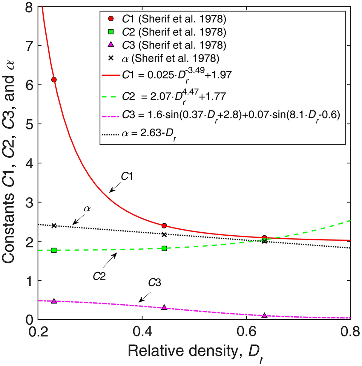
Ishibashi et al. (1977) and Sherif et al. (1978) investigated the behavior of Ottawa sand under uniform cyclic loading using the torsional simple shear device, and found that the ratio of the normalized incremental excess pore water pressure (

Δ U_{N}

) to the stress history function (

1 - U_{N - 1}

) is linearly related to the ratio of the shear stress (

τ_{N}

) during the current stress cycle to the effective pressure (

σ_{N - 1}^{'}

) from the previous stress cycle in a log-log plot. Ishibashi et al. (1977) and Sherif et al. (1978) proposed that the relationship can take the form of a power regression as given in Eq. (3), which is the governing equation of the original pore pressure model introduced in this study. The slope is denoted

α

, and is the power of the stress ratio (

τ_{N} / σ_{N - 1}^{'}

) in Eq. (3). Furthermore,

α

is considered to be constant at every cycle. The constant multiplier in Eq. (3) is denoted

\bar{N}

, which characterizes the effect of the number of stress cycles. In the original pore pressure model (Ishibashi et al. 1977; Sherif et al. 1978), a relationship between

\bar{N}

and

N

was proposed using three constants, namely

C 1

,

C 2

, and

C 3

[Eq. (4)]. The values of the these constants for loose, medium dense, and dense Ottawa sand were provided by Sherif et al. (1978), and are summarized in Fig. 3. To generalize the behavior of Ottawa sand, the relationships of the constants

C 1

,

C 2

,

C 3

, and

α

at various relative densities (

D_{r}

) also are shown in Fig. 3. The correlations of the constants with

D_{r}

, as proposed in this study, are given by Eqs. (5)–(8). Combining Eqs. (5)–(7) into Eq. (4) results in Eq. (9), which allows for effect of the number of stress cycles to be determined easily at any value of

D_{r}

. Rearranging Eq. (3), and combining Eqs. (8) and (9) into Eq. (3), the normalized incremental excess pore pressure rise (

Δ U

) with each stress cycle at any density can be calculated using Eq. (10), which is the governing equation of the density-based pore pressure model proposed in this study

\frac{Δ U_{N}}{1 - U_{N - 1}} = \bar{N} {(\frac{τ_{N}}{σ_{N - 1}^{'}})}^{α}

(3)

\bar{N} = \frac{Δ U_{N} {(\frac{τ_{N}}{σ_{N - 1}^{'}})}^{α}}{(1 - U_{N - 1})} = \frac{C 1 \cdot N}{N^{C 2} - C 3}

(4)

C 1 = (0.025 \cdot D_{r}^{- 3.49} + 1.97)

(5)

C 2 = (2.07 \cdot D_{r}^{4.47} + 1.77)

(6)

C 3 = [1.6 \cdot \sin (0.37 \cdot D_{r} + 2.8) + 0.07 \cdot \sin (8.1 \cdot D_{r} - 0.6)]

(7)

α = 2.63 - D_{r}

(8)

\bar{N} = \frac{(0.025 \cdot D_{r}^{- 3.49} + 1.97) \cdot N}{N^{(2.07 \cdot D_{r}^{4.47} + 1.77)} - [1.6 \cdot \sin (0.37 \cdot D_{r} + 2.8) + 0.07 \cdot \sin (8.1 \cdot D_{r} - 0.6)]}

(9)

Δ U_{N} = (1 - U_{N - 1}) {(\frac{τ_{N}}{σ_{N - 1}^{'}})}^{2.63 - D_{r}} \cdot \frac{(0.025 \cdot D_{r}^{- 3.49} + 1.97) \cdot N}{N^{(2.07 \cdot D_{r}^{4.47} + 1.77)} - [1.6 \cdot \sin (0.37 \cdot D_{r} + 2.8) + 0.07 \cdot \sin (8.1 \cdot D_{r} - 0.6)]}

(10)

Fig. 3. Relationship of $C 1$ , $C 2$ , $C 3$ , and $α$ with $D_{r}$ for Ottawa sand in torsional simple shear device.

Prediction of Pore Pressure Rise under Earthquake Loading

The number of cycles

N

in Eq. (10) is applicable only for uniform cyclic loading, and during an earthquake the shear stress amplitudes are irregular from one cycle to another. To evaluate all the numbers of cycles of different stress amplitudes prior to the cycle at which the pore pressure is to be predicted, variable

N

in Eq. (10) is replaced by the equivalent number of cycles

(N_{eq})

, and the shear stresses are considered independently in the positive and negative regions. In addition, the magnitudes of the pore pressures are determined solely by the value of the maximum shear stress in the half-cycle, because it has the most significant influence on pore-pressure buildup (Sherif et al. 1978). Hence, at the

N

th cycle, the maximum shear stress amplitudes from the first cycle to the

N

th cycle of the positive region determine the positive equivalent number of cycles

(N_{eq, p})

, whereas the maximum shear stress amplitudes of the negative region determine the negative equivalent number of cycles

(N_{eq, n})

[Eq. (11)]. In Eq. (11),

τ_{N, p}

is the positive cyclic shear stress during the

N

th cycle, and

τ_{N, n}

is the negative cyclic shear stress during the

N

th cycle. Due to asymmetry in the peak values during one cycle, pore pressure rise is predicted for every half-cycle. The normalized incremental excess pore pressure rise due to positive cyclic shear stress

τ_{N, p}

during the

N

th cycle (

Δ U_{N, p}

) is calculated using Eq. (12), whereas the normalized incremental excess pore pressure rise due to negative cyclic shear stress

τ_{N, n}

during the

N

th cycle (

Δ U_{N, n}

) is calculated using Eq. (13). The normalized total excess pore water pressure (

U_{N}

) during the

N

th cycle of an earthquake is expressed by Eq. (14)

N_{e q, p} = \sum_{i = 1}^{N} {(\frac{τ_{i, p}}{τ_{N, p}})}^{α}; N_{e q, n} = \sum_{i = 1}^{N} {(\frac{τ_{i, n}}{τ_{N, n}})}^{α}

(11)

Δ U_{N, p} = (1 - U_{N - 1}) {(\frac{τ_{N, p}}{σ_{N - 1}^{'}})}^{2.63 - D_{r}} \cdot \frac{(0.025 \cdot D_{r}^{- 3.49} + 1.97) \cdot N_{eq, p}}{N_{eq, p}^{(2.07 \cdot D_{r}^{4.47} + 1.77)} - [1.6 \cdot \sin (0.37 \cdot D_{r} + 2.8) + 0.07 \cdot \sin (8.1 \cdot D_{r} - 0.6)]}

(12)

Δ U_{N, n} = (1 - U_{N - 1}) {(\frac{τ_{N, n}}{σ_{N - 1}^{'}})}^{2.63 - D_{r}} \cdot \frac{(0.025 \cdot D_{r}^{- 3.49} + 1.97) \cdot N_{eq, n}}{N_{eq, n}^{(2.07 \cdot D_{r}^{4.47} + 1.77)} - [1.6 \cdot \sin (0.37 \cdot D_{r} + 2.8) + 0.07 \cdot \sin (8.1 \cdot D_{r} - 0.6)]}

(13)

U_{N} = U_{N - 1} + 0.5 (Δ U_{N, p} + Δ U_{N, n})

(14)

Calibration of Density-Based Pore Pressure Model

Triggering liquefaction curves in the literature usually are established from a baseline curve developed from the behavior of clean sand, a soil that contains little to no fines. The curve is derived based on an initial stress level close to the value of the atmospheric pressure, which is approximately 100 kPa, and based on the cyclic resistance ratio against a magnitude (

M_{w}

) 7.5 earthquake, which is approximately equivalent to the cyclic stress ratio (

τ / σ_{0}^{'}

) that can cause liquefaction in about 15 cycles (Seed and Idriss 1982). Liquefaction resistance is depicted by the relationship between cyclic stress ratio and the number of load cycles required to reach a liquefaction criterion, which usually is stress-based or strain-based (Yu et al. 2022). For example, Beaty and Byrne (2011) assumed that liquefaction occurs either if the normalized total excess pore water pressure (

U

) exceeds 0.85 or when the maximum shear strain exceeds 3%. Because the current pore pressure model cannot evaluate the shear strains, the complete liquefaction criteria was utilized in the calibration of the pore pressure model to symbolize a clear occurrence of liquefaction. As discussed in the Introduction, the original pore pressure model results in higher resistance to liquefaction at low densities and weaker resistance at high densities, and hence a method must be applied so that the liquefaction resistance can be adjusted to match that of the clean sand.

Calibration of Pore Pressure Model Based on Behavior of Clean Sand in Direct Simple Shear Tests

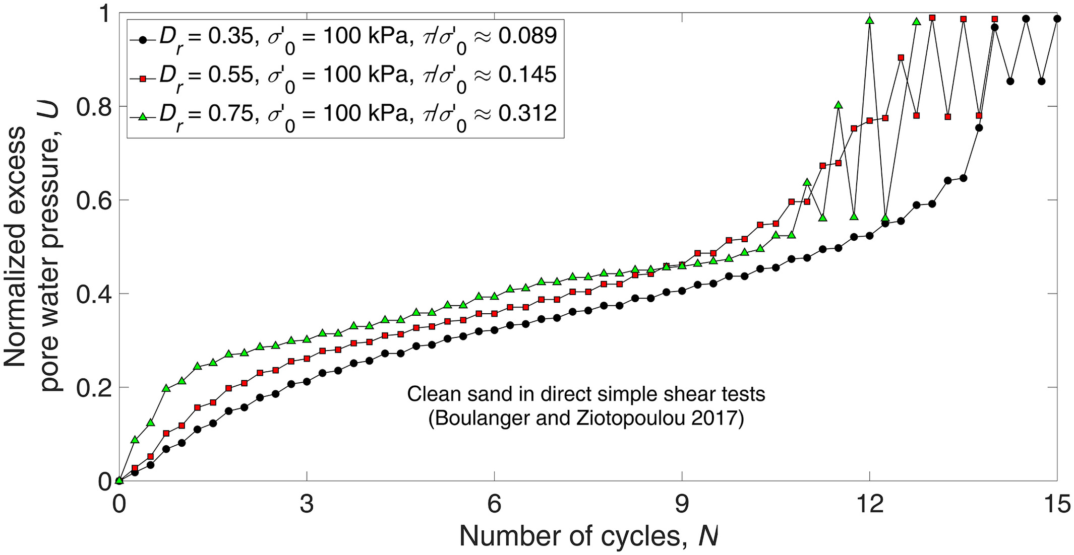
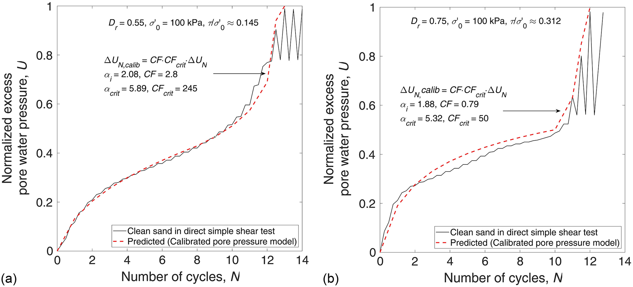
The first step is to calibrate the pore pressure model based on the behavior of clean sand in direct simple shear tests, as presented by Boulanger and Ziotopoulou (2017). The pore pressure–time history curves at relative densities (

D_{r}

) of 0.35, 0.55, and 0.75 and at cyclic shear loading (

τ / σ_{0}^{'}

) of 0.089, 0.145, and 0.312, respectively, are shown in Fig. 4. The shapes of the curves and the numbers of cycles to complete liquefaction differ. Hence, there is a need to investigate the characteristics that define the shape of the pore pressure–time history curve so as to be able to replicate the behavior of clean sand.

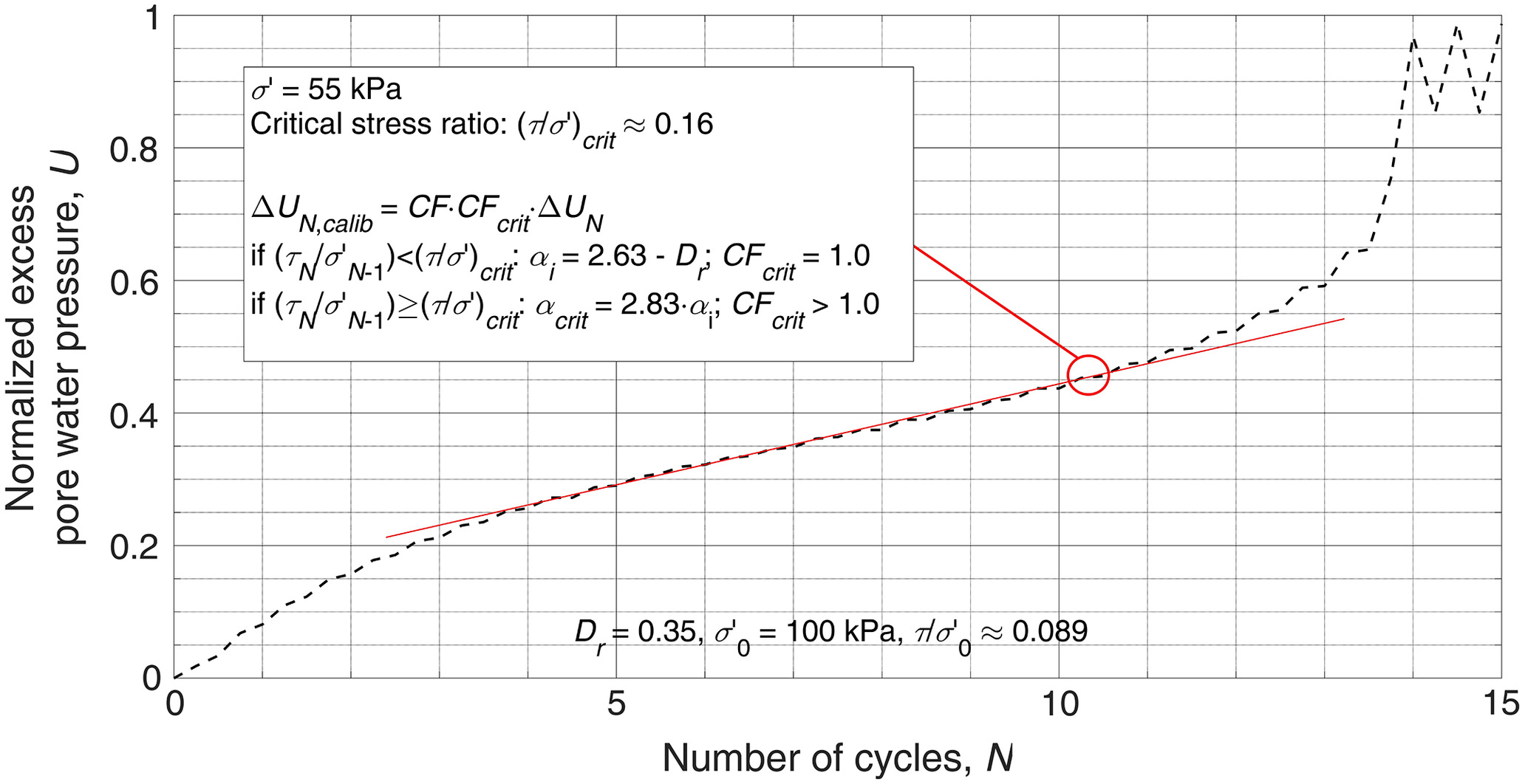
Fig. 4. Behavior of clean sand in direct simple shear tests at relative densities ( $D_{r}$ ) of 0.35, 0.55, and 0.75 with cyclic shear loading ( $τ / σ_{0}^{'}$ ) at 0.089, 0.145, and 0.312, respectively.

This study introduces calibration factors CF and

{CF}_{crit}

to adjust the original predicted curve of the pore pressure model (precalibrated curve), as shown in Eq. (15). Factor CF is applied to each incremental pore pressure rise per half-cycle throughout the duration of cyclic loading, whereas

{CF}_{crit}

is applied only when (

τ_{N} / σ_{N - 1}^{'}

) is greater than or equal to the critical stress ratio

(τ / σ^{'})_{crit}

. In this study,

(τ / σ^{'})_{crit}

is defined as the stress ratio at the start of the stage wherein the rate of excess pore water pressure accumulation starts to increase and diverges from the nearly constant rate of pore pressure buildup from the previous stage (Sherif et al. 1977; Konstadinou and Georgiannou 2014). The critical stress ratio

(τ / σ^{'})_{crit}

is determined by drawing a line on the graph that intersects with the portion in which the rate of pore pressure buildup is constant. The stress ratio that last intersects the line is determined to be the critical stress ratio (Fig. 5). In Fig. 5, when the effective stress is reduced to 55 kPa from an initial effective stress of 100 kPa due to a uniform cyclic shear loading of 8.9 kPa, the rate of pore pressure buildup starts to deviate and increase rapidly from a

U

of 0.45 to a

U

of about 0.98 in less than 3.0 s. For clean sand with

D_{r} = 0.35

, the critical stress ratio was determined to be approximately 0.16

Δ U_{N, calib} = CF \cdot {CF}_{crit} \cdot Δ U_{N}

(15)

Fig. 5. Determination of $(τ / σ^{'})_{crit}$ for clean sand at $D_{r} = 0.35$ .

When (

τ_{N} / σ_{N - 1}^{'}

) exceeds

(τ / σ^{'})_{crit}

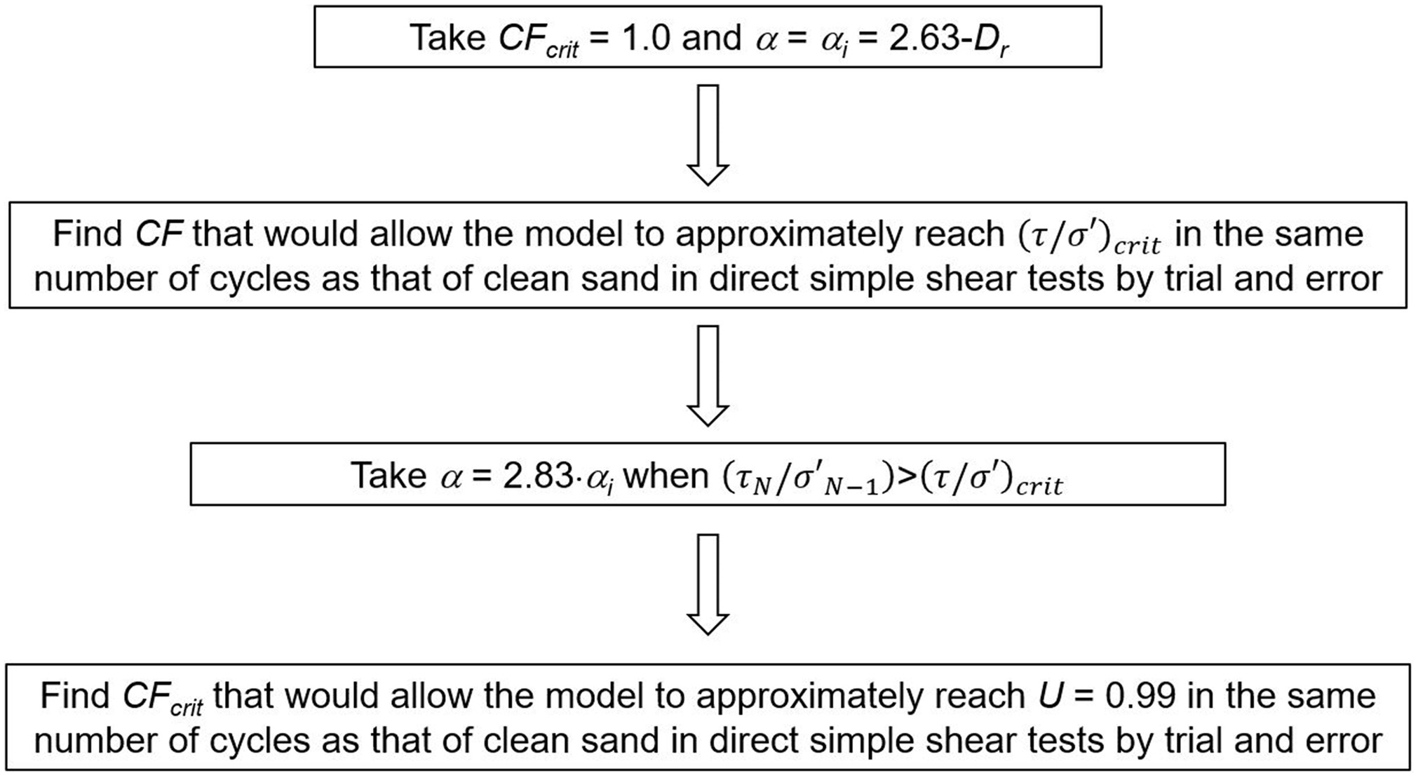
, the values of two parameters in the pore pressure model, namely

α

and

{CF}_{crit}

, are changed. Konstadinou and Georgiannou (2014) deduced that the value of

α

increases by about 2.83 times the initial value of

α

when (

τ_{N} / σ_{N - 1}^{'}

) is greater than

(τ / σ^{'})_{crit}

. They presented the change in

α

when the stress ratio exceeded the critical stress ratio for Ham river sand with a relative density of 35%. They showed that an increase of

α

to 6.8 from a value of 2.4 was satisfactory for the observed behavior. Their analysis included not only Ham river sand but also Fontainebleau sand, M31 sand, and Ottawa sand, and the densities of the tested soils ranged from 19% to 61%. The initial value of

α

is denoted as

α_{i}

and has a value given by Eq. (8), and

α_{i}

multiplied by 2.83 is denoted

α_{crit}

[Eq. (16)]. This change in

α

allows for the rate of pore pressure rise to transition slowly to a rapid rate after

(τ / σ^{'})_{crit}

is achieved. The value of

{CF}_{crit}

is 1.0 when (

τ_{N} / σ_{N - 1}^{'}

) is less than

(τ / σ^{'})_{crit}

, and it increases to a value greater than 1.0 when (

τ_{N} / σ_{N - 1}^{'}

) is greater than or equal to

(τ / σ^{'})_{crit}

. The value of

{CF}_{crit}

is determined by following the steps in Fig. 6

α_{crit} = 2.83 \cdot α_{i}

(16)

Fig. 6. Procedure for determining the value of ${CF}_{crit}$ .

Based on the data in Fig. 4, the values of

(τ / σ^{'})_{crit}

were determined for

D_{r} = 0.55

and

D_{r} = 0.75

(Fig. 7);

(τ / σ^{'})_{crit}

increased with relative density. This study assumed that

(τ / {σ^{'})}_{crit}

is density-dependent. This attribute was presented by Konstadinou and Georgiannou (2014), who showed that

(τ / σ^{'})_{crit}

can be assumed to be constant at various shear loading magnitudes. In this study, the critical stress ratio was correlated with the peak stress ratio

(τ / σ^{'})_{p e a k}

to widen the scope of parameters considered by the pore pressure model. The peak stress ratios can be estimated based on either the peak friction angle (

ϕ_{peak}

) using the equation

(τ / σ^{'})_{peak} = \sin (ϕ_{peak})

, or the critical-state approach introduced by Boulanger and Ziotopoulou (2017). For the pore pressure model, the critical state approach is recommended because it considers the constant friction angle (

ϕ_{c v}

) and the relative state parameter index (

ξ_{r}

). The parameter

ϕ_{c v}

affects the dilative and contractive behavior of the soil because it controls the boundary between dilation and contraction. Elgamal et al. (1998) reported the possibility of the influence of soil-skeleton dilation on the shear stiffness and shear strength, and they suggested that phases of dilation can lead to instances of pore pressure reduction, spikes in lateral acceleration records, and strong restraining effect on shear strains.

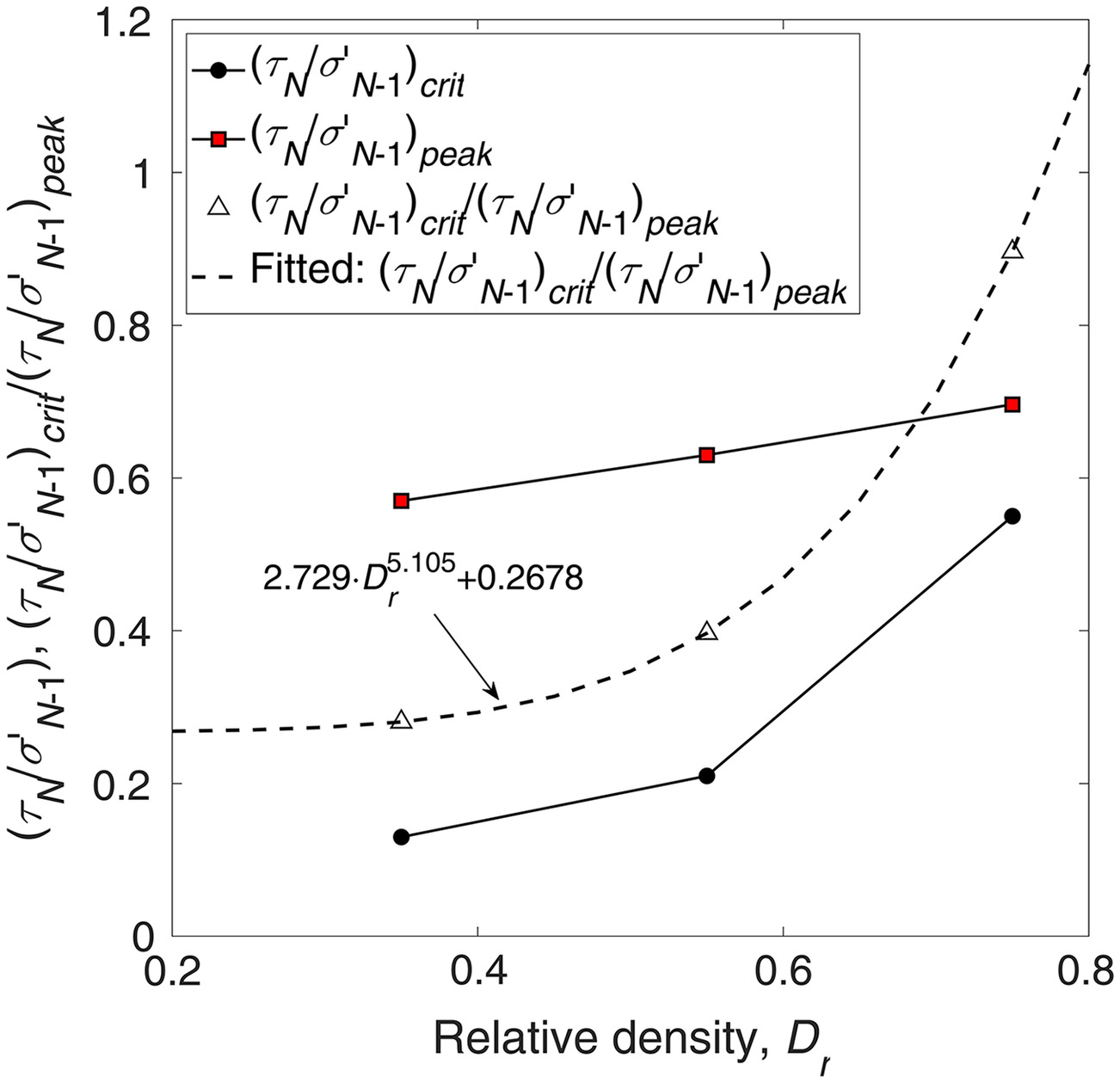
Fig. 7. Variation of $(τ / σ^{'})_{crit}$ , $(τ / σ^{'})_{peak}$ , and $(τ / {σ^{'})}_{crit} / (τ / σ^{'})_{peak}$ with relative density for clean sand.

The peak stress ratios for

D_{r} = 0.35

, 0.55, and 0.75 were determined based on the method by Boulanger and Ziotopoulou (2017) (Fig. 7). To relate the critical stress ratio to the peak stress ratio,

(τ / σ^{'})_{crit} / (τ / σ^{'})_{peak}

versus relative density was determined (Fig. 7). The value of

(τ / σ^{'})_{crit} / (τ / σ^{'})_{peak}

increased nonlinearly with the increase of relative density. As a result, Eq. (17) is proposed to determine

(τ / σ^{'})_{crit}

based on

D_{r}

and

(τ / σ^{'})_{peak}

. Boulanger and Ziotopoulou (2017) suggested that the default value of

ϕ_{c v}

for clean sand is 33°, and the default value of

n^{b}

is 0.5 when

ξ_{r} < 0

, and 0.125 when

ξ_{r} > 0

. Currently, the pore pressure model has been calibrated using only a constant friction angle of 33°; hence, further analysis and validation using constant friction angles other than 33° degrees are recommended

{(τ / σ^{'})}_{crit} = (2.729 \cdot D_{r}^{5.105} + 0.2678) \cdot {(τ / σ^{'})}_{peak} = (2.729 \cdot D_{r}^{5.105} + 0.2678) [0.5 \cdot \sin (ϕ_{c v}) \cdot \exp (- n^{b} \cdot ξ_{r})]

(17)

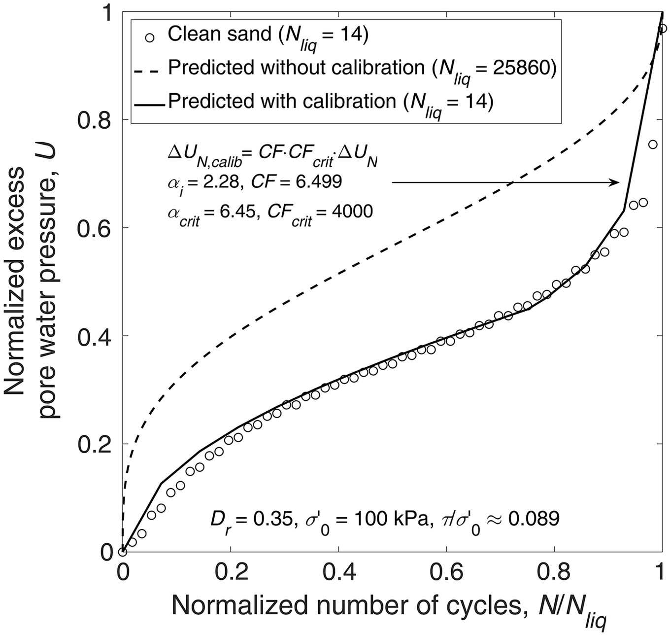
Sample calibration of the pore pressure model based on the behavior of clean sand with

D_{r} = 0.35

is shown in Fig. 8. The number of cycles was normalized with the number of cycles to complete liquefaction

(N_{liq})

to differentiate the curves of the model without calibration and the calibrated model. The model without calibration is notably more resistant to liquefaction at lower densities; therefore it took an excessive number of cycles to achieve complete liquefaction. Furthermore, the predicted curve without calibration overestimated the normalized excess pore water pressure with the normalized number of cycles. Introducing CF,

{CF}_{crit}

, and

α_{crit}

into the pore pressure model and using values of 6.499, 4,000, and 6.45, respectively, resulted in good agreement with the clean sand, which liquefied in only 14 cycles, compared with the original pore pressure model which predicted complete liquefaction after 25,860 cycles. The values of

{CF}_{crit}

for

D_{r} = 0.55

and 0.75 also were determined (Fig. 9). Based on Fig. 9, Eq. (18) is proposed as a means to relate

{CF}_{crit}

to

D_{r}

. Simulations of the calibrated pore pressure model using the suggested values of

α_{crit}

and

{CF}_{crit}

are shown in Fig. 10. The calibrated pore pressure model adequately predicted the behavior of clean sand at

D_{r} = 0.55

and

D_{r} = 0.75

. The value of CF for

D_{r} = 0.75

is less than 1.0. This is because the original pore pressure model has low resistance to liquefaction at higher densities; therefore a CF value less than 1.0 will decelerate the rise in pore pressure

{CF}_{crit} = 5.121 \cdot D_{r}^{- 6.34} + 18.27

(18)

Fig. 8. Sample calibration of the pore pressure model for $D_{r} = 0.35$ .

Fig. 9. Variation of ${CF}_{crit}$ with relative density ( $D_{r}$ ).

Fig. 10. Behavior comparison of clean sand in direct simple shear test and calibrated pore pressure model: (a) $D_{r} = 0.55$ ; and (b) $D_{r} = 0.75$ .

Calibration Based on Triggering Liquefaction Curves

In the section “Calibration of Pore Pressure Model Based on Behavior of Clean Sand in Direct Simple Shear Tests,” the focal point of calibration was the determination of the critical stress ratio and its influence on the shape of the excess pore-water pressure curve, whereas in this section, the pore pressure model is calibrated based on sets of CRR curves from well-known triggering liquefaction curves. The CRR can be obtained from the pore pressure model by setting the target number of cycles, and the (

τ / σ_{0}^{'}

) that can cause liquefaction at the target number of cycles is determined as the CRR. The overall CF obtained from the previous section is related to the calibration factor for a magnitude 7.5 earthquake (

{CF}_{7.5}

), the calibration factor ratio for earthquake magnitude or number of cycles to liquefaction (

{CFratio}_{N liq}

), and the calibration factor ratio for the initial effective stress (

{CFratio}_{σ^{'}}

), as shown in Eq. (19). In this study, the CFratio is defined as the ratio of the overall CF to

{CF}_{7.5}

[Eq. (20)]. Utilizing CFratio allows multiple influential parameters that affect the cyclic strength of the soil to be integrated into the pore pressure model

CF = {CF}_{7.5} \cdot {CFratio}_{N liq} \cdot {CFratio}_{σ^{'}}

(19)

CFratio = \frac{CF}{{CF}_{7.5}}

(20)

Calibration Based on Clean Sand Base Curve

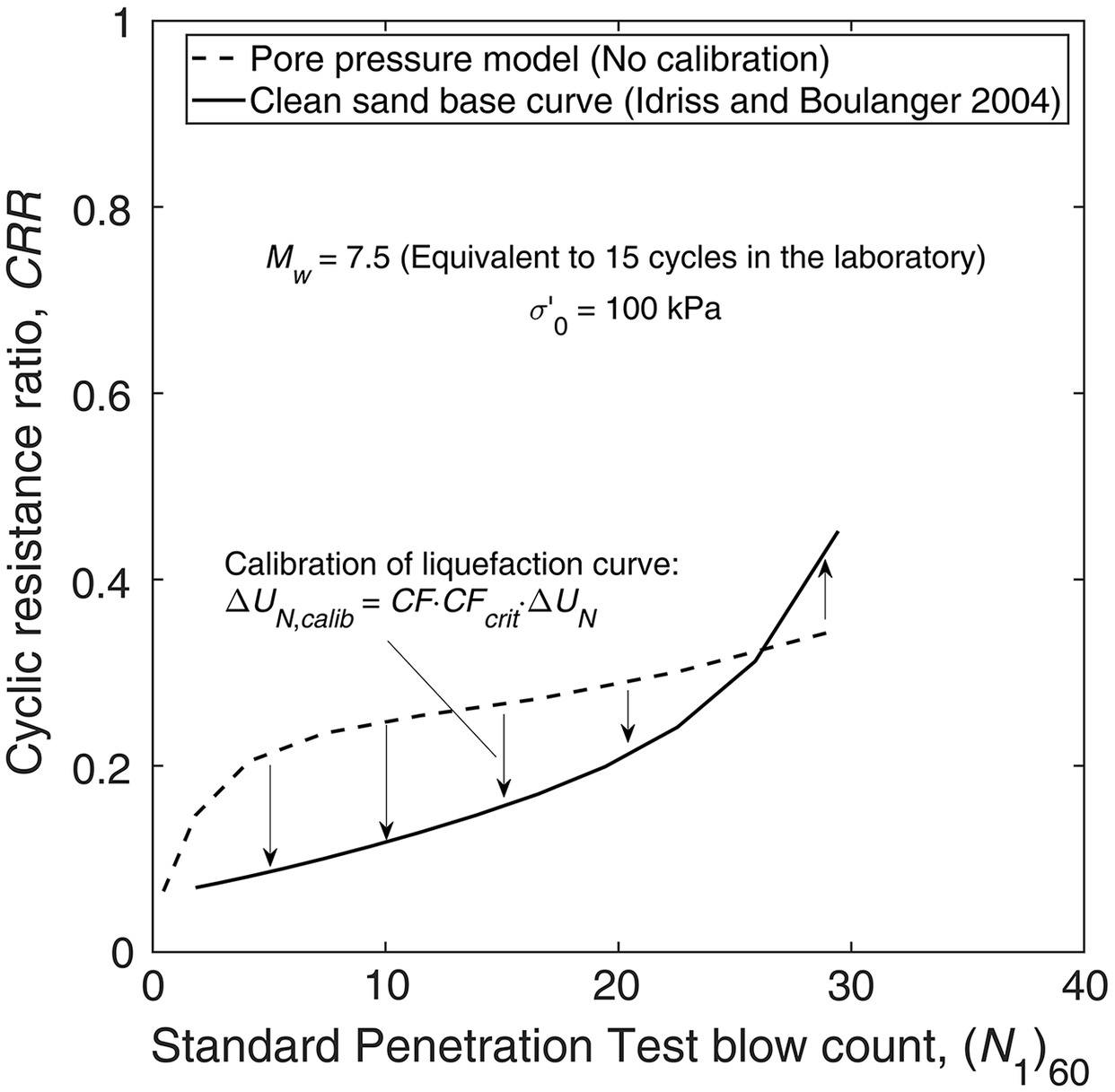
Idriss and Boulanger (2004) re-examined the semiempirical procedures for evaluating the liquefaction potential of saturated cohesionless soils during earthquakes, and proposed Eq. (21) to determine the value of the cyclic resistance ratio of clean sand for a magnitude 7.5 earthquake (

{CRR}_{7.5}

) at an initial effective stress (

σ_{0}^{'}

) of 100 kPa. Because the pore pressure model is derived based on relative density, the relation in Eq. (22), which was suggested by Boulanger and Ziotopoulou (2017), is used to convert the SPT blow count

(N_{1})_{60}

to its corresponding value of

D_{r}

. By integrating CF and

{CF}_{crit}

into the pore pressure model, it is possible to adjust the cyclic strength curve shown in Fig. 11. For an earthquake of

M_{w} = 7.5

,

N_{liq}

is set to 15, which is the value proposed by Seed and Idriss (1982). Consequently, calibration of the pore pressure model is possible based on the complete liquefaction criterion. The CRRs at blow counts lower than 26 need to be reduced, whereas the CRR at blow counts greater than 26 need to be shifted upward to match the clean-sand base curve

{CRR}_{7.5} = \exp [\frac{{(N_{1})}_{60}}{14.1} + {(\frac{{(N_{1})}_{60}}{126})}^{2} - {(\frac{{(N_{1})}_{60}}{23.6})}^{3} + {(\frac{{(N_{1})}_{60}}{25.4})}^{4} - 2.8]

(21)

D_{r} = \sqrt{\frac{{(N_{1})}_{60}}{46}}

(22)

Fig. 11. CRR adjustment of original pore pressure model using calibration factor (CF).

To obtain

{CF}_{7.5}

, other influential parameters, including

{CFratio}_{N liq}

and

{CFratio}_{σ^{'}}

, must be set to 1.0. A value of 1.0 for

{CFratio}_{N liq}

means that the shear loading is equivalent to an earthquake with a moment magnitude (

M_{w}

) of 7.5, and a value of 1.0 for

{CFratio}_{σ^{'}}

means that the initial effective stress (

σ_{0}^{'}

) is 100 kPa. When

M_{w}

and

σ_{0}^{'}

values are other than the baseline values, CFratio can be either less than or greater than 1.0. Furthermore, the values of

{CF}_{crit}

in terms of relative density [Eq. (18)] are not adjusted in the calibration process. Because

{CRR}_{7.5}

for a relative density is already known from Eq. (21), the values of

{CF}_{7.5}

are to be determined by trial and error, which can be a tedious method. To accelerate the determination of

{CF}_{7.5}

with relative density and

{CRR}_{7.5}

, the pore pressure model was coded in MATLAB Version R2019b such that

{CF}_{7.5}

increases from 0 to 12 until the value of

U

at 15 cycles is equal to or greater than 0.99. In other words, when the predicted

U

after 15 cycles is less than 0.99, the previous value of

{CF}_{7.5}

is increased incrementally, and the pore pressure rise from

N = 1

to 15 is calculated again until the failure criterion is satisfied. To ensure that the obtained value of

{CF}_{7.5}

is satisfactory, it is necessary to use smaller increments; however, very small increments could result in longer calculation times.

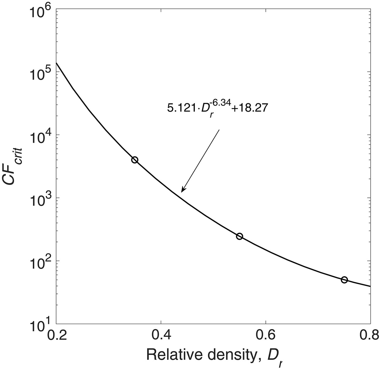
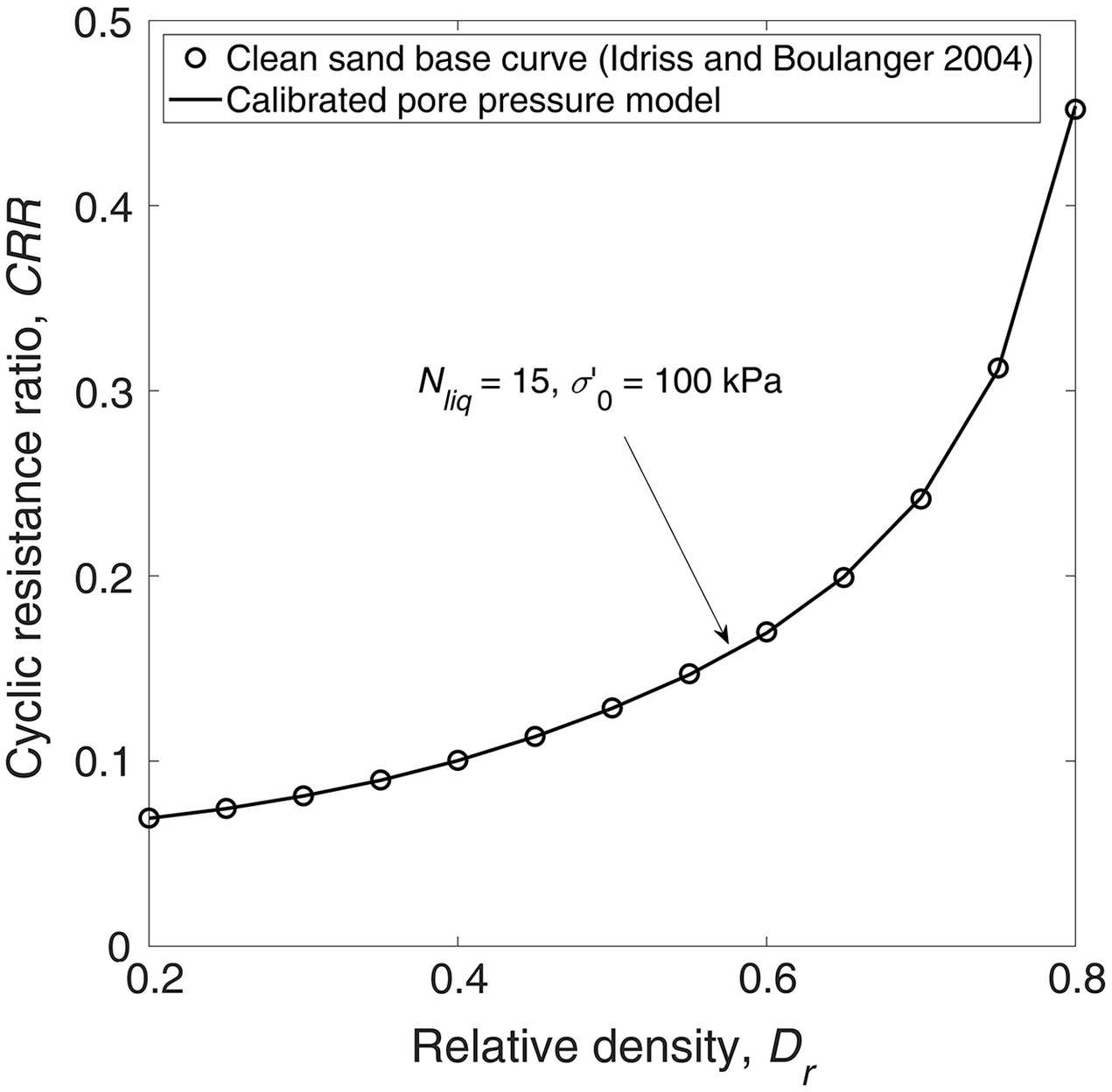
The values of

{CF}_{7.5}

with relative density, which were obtained by trial and error, are shown in Fig. 12. The value of

{CF}_{7.5}

increased nonlinearly with relative density from 5.0 to about 6.8, and decreased substantially to less than 1.0 when

D_{r} > 0.75

. Due to the high nonlinearity of the relationship between

D_{r}

and

{CF}_{7.5}

, the rational function in Eq. (23) is proposed such that

{CF}_{7.5}

can be obtained for any value of

D_{r}

. Utilizing Eq. (23) and setting the number of cycles to 15, the predicted CRR from the pore pressure model had very good agreement with the clean-sand base curve (Fig. 13)

{CF}_{7.5} = (\frac{- 34.13 \cdot D_{r}^{4} + 74.1 \cdot D_{r}^{3} - 59.47 \cdot D_{r}^{2} + 19.86 \cdot D_{r} - 1.621}{D_{r}^{2} - 0.456 \cdot D_{r} + 0.1523})

(23)

Fig. 12. Variation of ${CF}_{7.5}$ with relative density.

Fig. 13. Comparison of clean sand base curve and calibrated pore pressure model.

Calibration Considering Magnitude Scaling Factor or Number of Cycles to Liquefaction

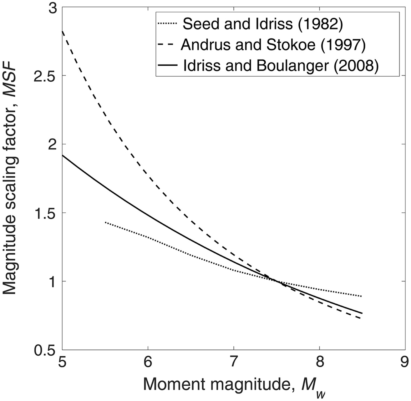
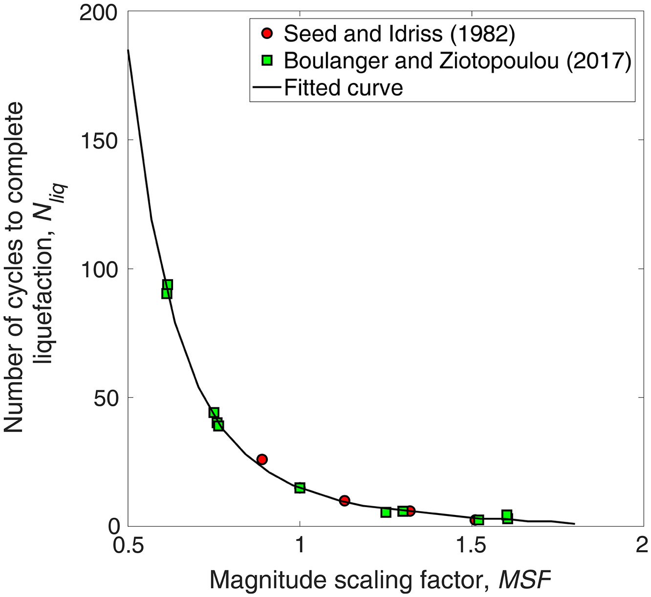
Numerous researchers, including Seed and Idriss (1982), Andrus and Stokoe (1997), and Idriss and Boulanger (2008), have suggested values of magnitude scaling factors (MSFs) with moment magnitude (

M_{w}

) (Fig. 14). These values of MSF are multiplied with

{CRR}_{7.5}

to obtain the

{CRR}_{Mw}

of the soil at various earthquake magnitudes [Eq. (24)]. To calibrate the pore pressure model considering the effect of earthquake magnitude, it is necessary to determine the equivalent number of cycles to liquefaction

(N_{liq})

. This is because the calibration method proposed in this study is based on failure at a target number of cycles. Instead of relating

N_{liq}

to

M_{w}

, the

N_{liq} - MSF

relationship is suggested due to the variations of relationship between MSF and

M_{w}

in the literature. For

M_{w} = 6.0

, the MSF values from Seed and Idriss (1982), Andrus and Stokoe (1997), and Idriss and Boulanger (2008) range between 1.3 and 1.9 (Fig. 14). In the present study, the relationship between MSF and

N_{liq}

was obtained from Seed and Idriss (1982) and from Boulanger and Ziotopoulou (2017), and the data are summarized in Fig. 15. Curve fitting was performed, and the relationship in Eq. (25) is proposed to calculate

N_{liq}

based on the MSF

{CRR}_{Mw} = MSF \times {CRR}_{7.5}

(24)

N_{liq} = 7900 \cdot \exp (- 8.122 \cdot MSF) + 187.5 \cdot \exp (- 2.69 \cdot MSF)

(25)

Fig. 14. MSF with moment magnitude ( $M_{w}$ ).

Fig. 15. Relationship between MSF and $N_{liq}$ .

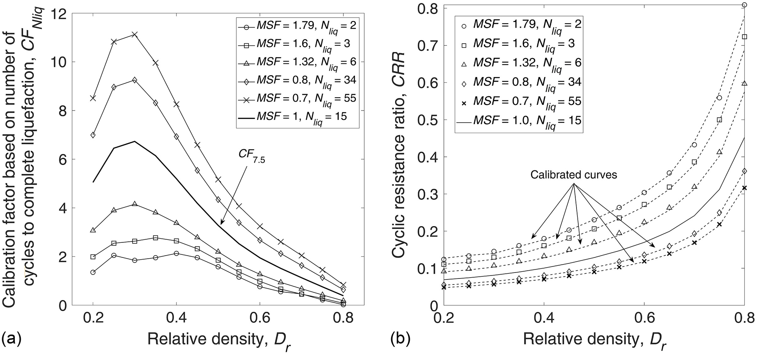
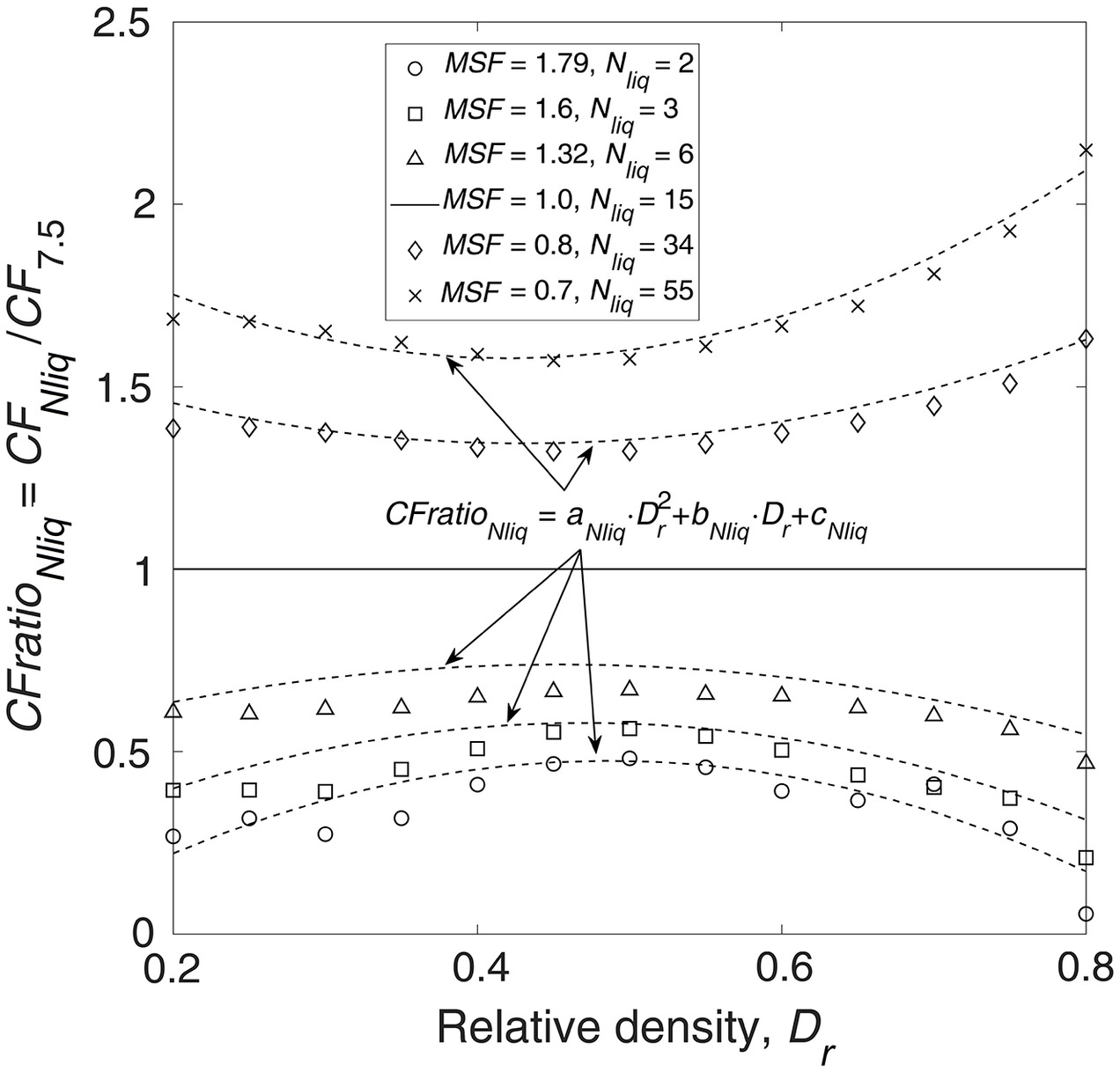
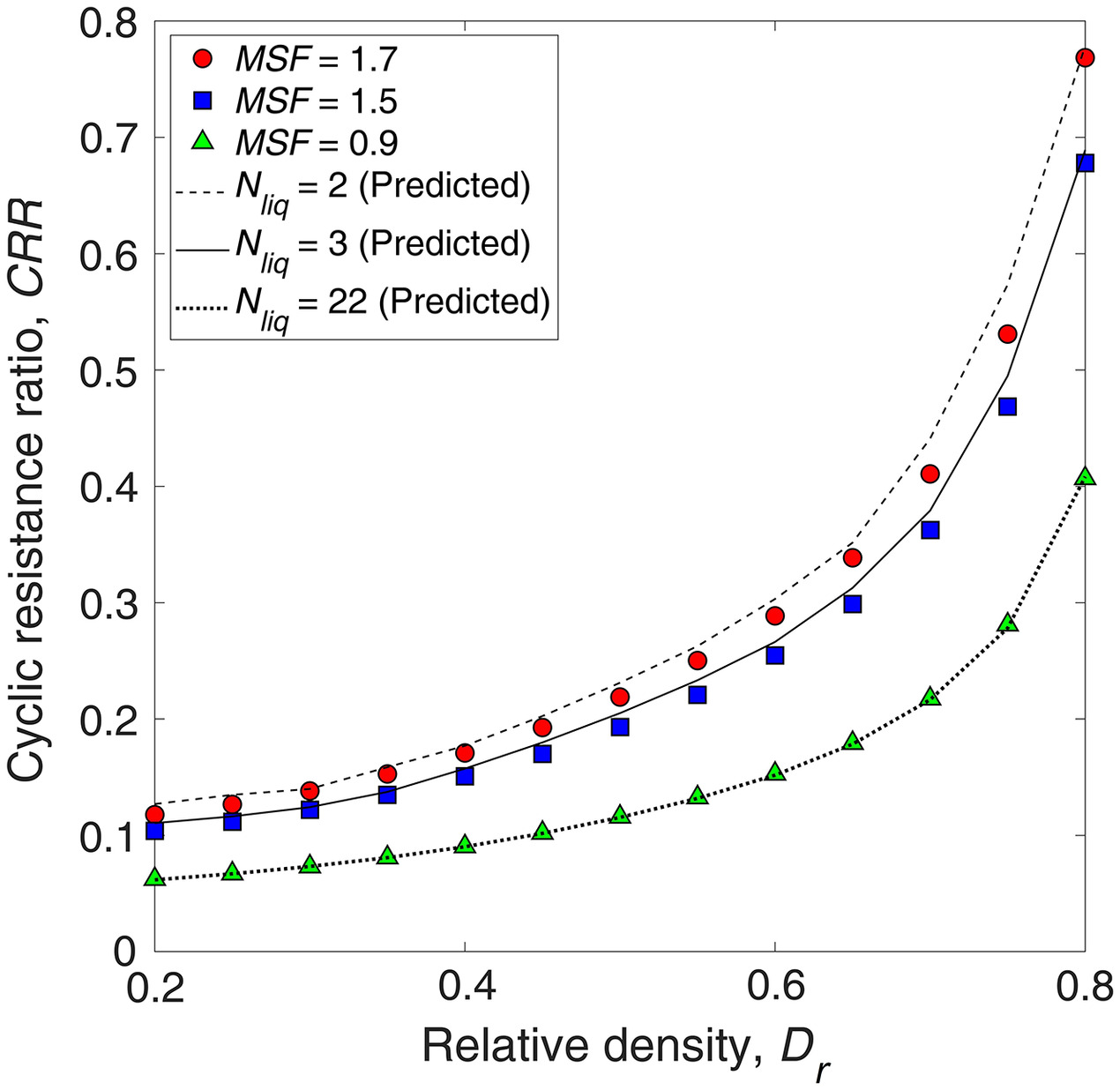
Setting the MSF to 1.79, 1.6, 1.32, 0.8, and 0.7, and setting

N_{liq}

to 2, 3, 6, 34, and 55, respectively,

{CF}_{N liq}

was obtained for relative densities ranging between 0.2 and 0.8 [Fig. 16(a)]. The calibrated curves using

{CF}_{N liq}

from Fig. 16(a) are shown in Fig. 16(b). In the calibration,

{CF}_{N liq}

is equal to the overall CF by setting

σ_{0}^{'}

to 100 kPa, so that

{CFratio}_{σ^{'}}

is equal to 1.0, making it a nonfactor in the calibration. Dividing

{CF}_{N liq}

in Fig. 16(a) by

{CF}_{7.5}

, the variation of

{CFratio}_{N liq}

with

D_{r}

at various values of MSF and

N_{liq}

is obtained [Eq. (26) and Fig. 17]. It then was determined that

{CFratio}_{N liq}

can be related to

D_{r}

through a polynomial function given by Eq. (27), in which the values of

a_{N liq}

,

b_{N liq}

, and

c_{N liq}

can be obtained by relating them to

N_{liq}

using the rational functions in Eqs. (28)–(30), respectively. Using Eq. (27), the cyclic resistance curves obtained from the calibrated pore pressure model for

N_{liq} = 2

, 3, and 22 were compared with the cyclic resistance curve obtained using Eq. (24) for

MSF = 1.7

, 1.5, and 0.9. The data were in adequate agreement with each other (Fig. 18)

{CFratio}_{N liq} = \frac{{CF}_{N liq}}{{CF}_{7.5}}

(26)

{CFratio}_{N liq} = a_{N liq} \cdot D_{r}^{2} + b_{N liq} \cdot D_{r} + c_{N liq}

(27)

where

a_{N liq} = (\frac{10.15 \cdot N_{liq}^{2} - 161.1 \cdot N_{liq} + 80.88}{N_{liq}^{2} + 57 \cdot N_{liq} - 53.04})

(28)

b_{N liq} = (\frac{- 7.858 \cdot N_{liq}^{2} + 122.9 \cdot N_{liq} - 44.16}{N_{liq}^{2} + 48.44 \cdot N_{liq} - 44.3})

(29)

c_{N liq} = (\frac{4.065 \cdot N_{liq}^{2} + 0.8483 \cdot N_{liq} - 34.92}{N_{liq}^{2} + 46.68 \cdot N_{liq} - 31.37})

(30)

Fig. 16. Calibration of pore pressure model considering MSF and $N_{liq}$ : (a) variation of ${CF}_{N liq}$ with $D_{r}$ ; and (b) calibrated cyclic strength curves at various MSF and $N_{liq}$ .

Fig. 17. Variation of ${CFratio}_{N l i q}$ with $D_{r}$ at various MSF and $N_{liq}$ .

Fig. 18. CRR from Eq. (24) and from pore pressure model for $MSF = 1.7$ , 1.5, and 0.9.

Fig. 19. Calibration considering effect of $K_{σ}$ : (a) calibrated curves under various initial effective stresses; and (b) variation of ${CFratio}_{σ^{'}}$ with $D_{r}$ for various initial effective stresses.

Calibration Considering Influence of Initial Effective Stress

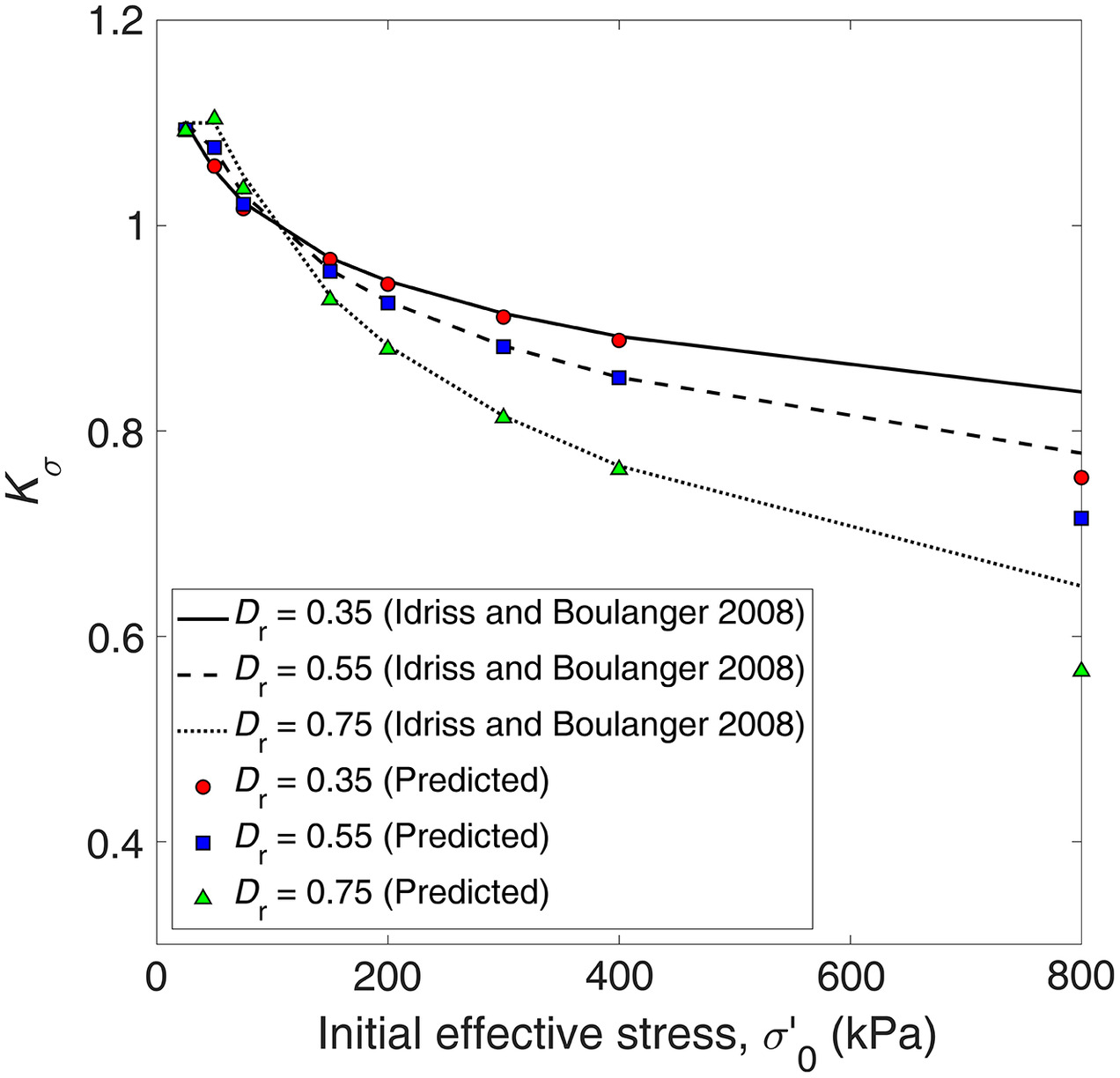
The cyclic resistance of a soil is influenced by the effective overburden stress. Seed (1981) introduced the overburden correction factor (

K_{σ}

) to adjust the CRR based on a common value of effective overburden stress. Relationships with

K_{σ}

have been derived from laboratory tests, theoretical considerations, and regression against field case histories, including those presented by Harder and Boulanger (1997), Hynes and Olsen (1998), Boulanger (2003), Boulanger and Idriss (2004), and Cetin et al. (2004). The recommended

K_{σ}

relationship expressed in terms of relative density and the cyclic resistance considering the influence of overburden effective stress (

{CRR}_{σ^{'}}

), as presented by Idriss and Boulanger (2008), is given in Eq. (31). Calibration was performed based on Eq. (31) [Fig. 19(a)]. In the calibration of the model, eight datasets of

{CF}_{σ^{'}}

from various initial effective stresses were obtained for relative densities ranging between 0.2 and 0.8. The value of

N_{liq}

was set to 15 cycles so that

{CFratio}_{N liq}

could be taken as 1.0. Then

{CFratio}_{σ^{'}}

was obtained using Eq. (32), and sample values of

{CFratio}_{σ^{'}}

for effective stresses 50, 200, 400, and 800 kPa are shown in Fig. 19(b). It was determined that

{CFratio}_{σ^{'}}

can be related to

D_{r}

by the power function in Eq. (32), wherein the values of

a_{σ^{'}}

,

b_{σ^{'}}

, and

c_{σ^{'}}

can be obtained using Eqs. (33)–(35), respectively. The

K_{σ}

values recommended by Idriss and Boulanger (2008) and those predicted by the calibrated pore pressure model are shown in Fig. 20. The data predicted by the calibrated pore pressure model were in fair agreement with the recommended values. In Fig. 20, values at 800 kPa differ because

K_{σ}

was adjusted to amplify slightly the influence of the initial effective stress at values greater than 400 kPa

{CRR}_{σ^{'}} = K_{σ} \cdot {CRR}_{7.5} = [1 - (\frac{1}{18.9 - 17.3 \cdot D_{r}}) \cdot \ln (\frac{σ_{0}^{'}}{100})] \cdot {CRR}_{7.5}

(31)

{CFratio}_{σ^{'}} = \frac{{CF}_{σ^{'}}}{{CF}_{7.5}} = a_{σ^{'}} \cdot D_{r}^{b_{σ^{'}}} + c_{σ^{'}}

(32)

If

σ_{0}^{'} \leq 100 kPa

a_{σ^{'}} = - 2.03 \times 10^{- 6} \cdot σ_{0}^{' 3} + 5.33 \times 10^{- 4} \cdot σ_{0}^{' 2} - 0.0412 \cdot σ_{0}^{'} + 0.8158

If

σ_{0}^{'} > 100 kPa

a_{σ^{'}} = 3.484 \times 10^{- 8} \cdot σ_{0}^{' 3} - 2.607 \times 10^{- 5} \cdot σ_{0}^{' 2} + 0.01114 \cdot σ_{0}^{'} - 0.8966

(33)

If

σ_{0}^{'} \leq 100 kPa

b_{σ^{'}} = - 7.17 \times 10^{- 5} \cdot σ_{0}^{' 3} + 0.0141 \cdot σ_{0}^{' 2} - 0.8101 \cdot σ_{0}^{'} + 15.598

If

σ_{0}^{'} > 100 kPa

b_{σ^{'}} = 1.877 \times 10^{- 9} \cdot σ_{0}^{' 3.161} + 3.601

(34)

If

σ_{0}^{'} \leq 100 kPa

c_{σ^{'}} = 0.1729 \cdot \ln (σ_{0}^{'}) + 0.206

If

σ_{0}^{'} > 100 kPa

c_{σ^{'}} = 5.3 \times 10^{- 9} \cdot σ_{0}^{' 3} - 5.832 \times 10^{- 6} \cdot σ_{0}^{' 2} + 0.002978 \cdot σ_{0}^{'} + 0.7555

(35)

Fig. 20. $K_{σ}$ values from Idriss and Boulanger (2008) and from calibrated pore pressure model.

Verification of Calibrated Pore Pressure Model

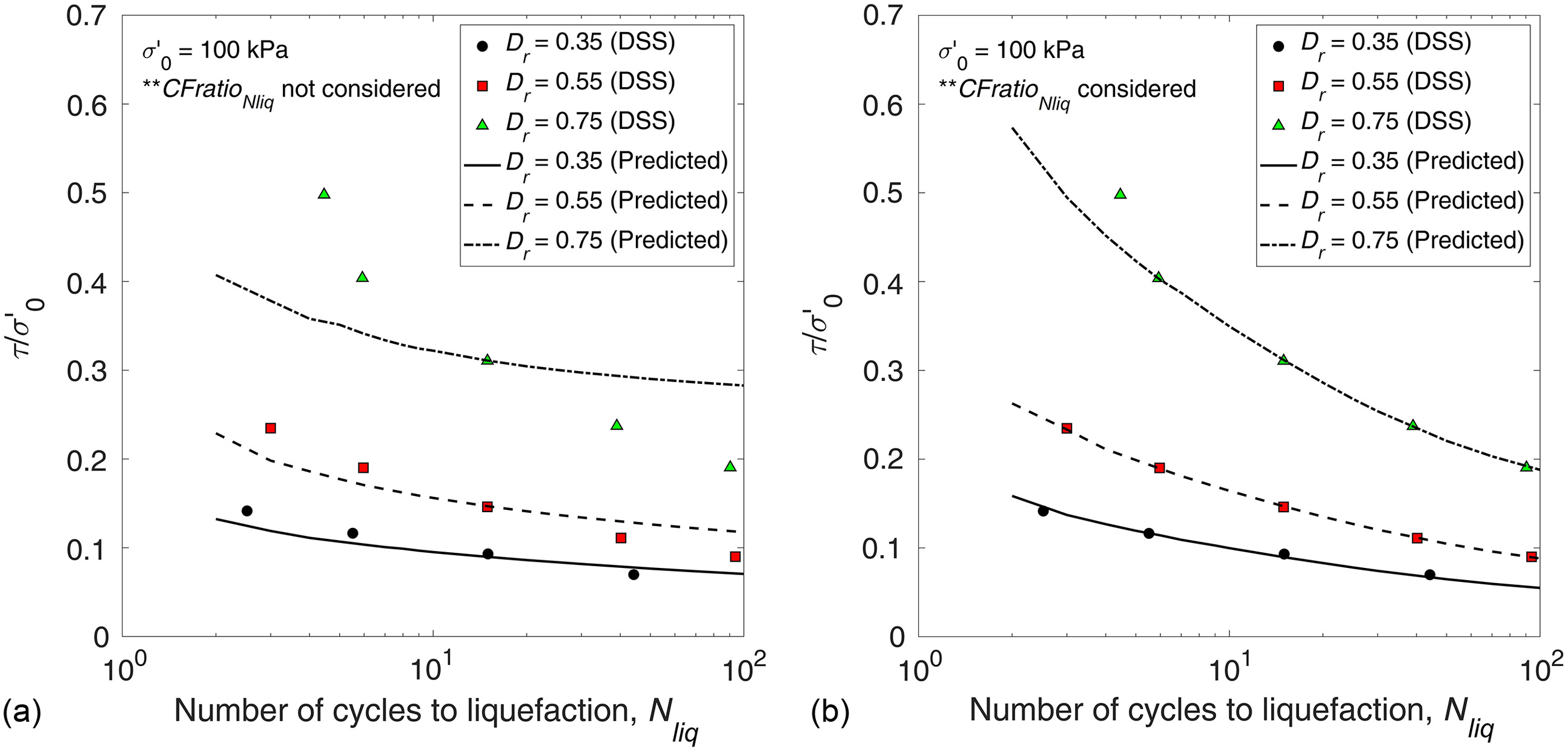
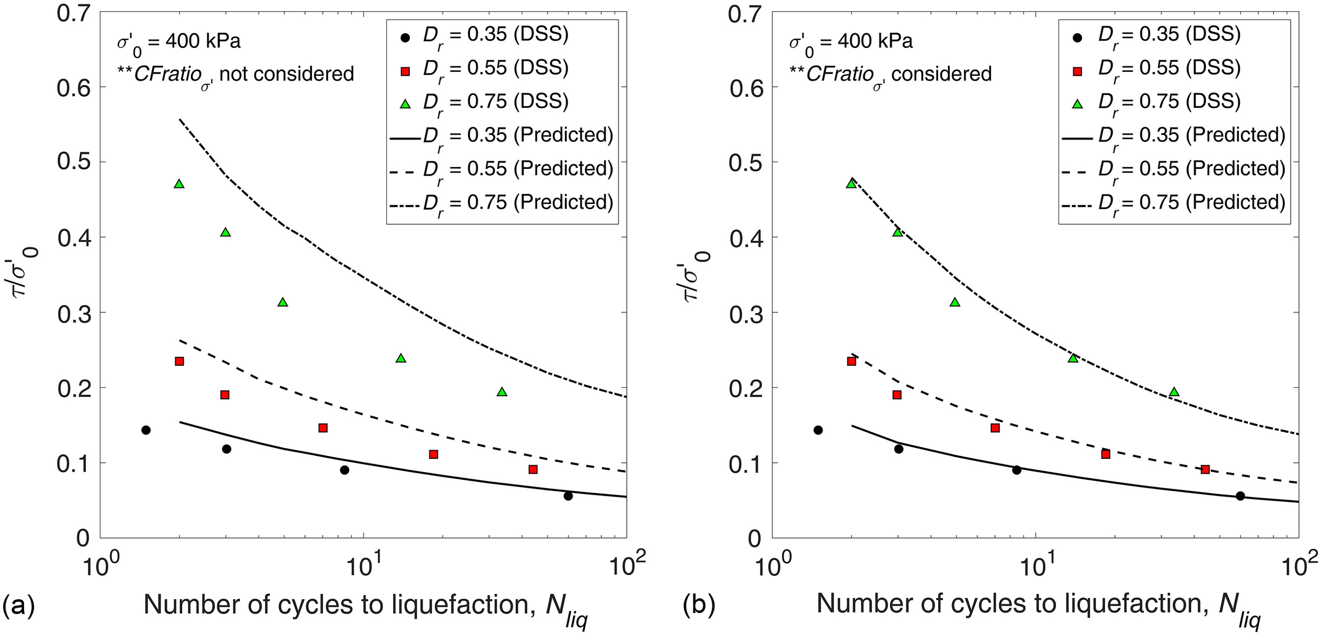
To verify the calibrated pore pressure model, the variation of

τ / σ_{0}^{'}

with

N_{liq}

was predicted and compared with the data presented by Boulanger and Ziotopoulou (2017) for clean sands in direct simple shear tests (DSS). The coefficient of earth pressure at rest (

K_{0}

) was 0.5 for the DSS data, which is the default value for the calibrated pore pressure model. In the calibrated pore pressure model,

K_{0}

is utilized in the calculation of the relative state parameter index (

ξ_{r}

). For reference, data from Boulanger and Ziotopoulou (2017) presented herein were based on failure at 3% shear strain, whereas the complete liquefaction criterion was used for the predicted data. In the simulations,

τ / σ_{0}^{'}

was predicted for

N_{liq}

ranging between 2 and 100. To verify

{CF}_{7.5}

and

{CFratio}_{N liq}

, the behavior of clean sand with an initial effective stress of 100 kPa is shown in Fig. 21. In Fig. 21(a), both

{CFratio}_{N liq}

and

{CFratio}_{σ^{'}}

are set to 1.0, whereas in Fig. 22(b)

{CFratio}_{N liq}

was obtained using Eq. (27). In both figures,

{CF}_{7.5}

was applied using Eq. (23). Disregarding

{CFratio}_{N liq}

resulted in a very clear disagreement with the DSS data at

D_{r} = 0.75

[Fig. 21(a)]. However, there was good agreement for

N_{liq} = 15

cycles, verifying Eq. (23). Using Eq. (27), the curves became steeper, resulting in better agreement with the DSS data [Fig. 21(b)]. To verify the calibrated pore pressure model considering the effect of

σ_{0}^{'}

, DSS data from Boulanger and Ziotopoulou (2017) for an initial effective stress of 400 kPa were compared with the predicted data obtained by the calibrated pore pressure model (Fig. 22). The pore pressure model that did not consider

{CFratio}_{σ^{'}}

resulted in the overestimation of the

τ / σ_{0}^{'}

that can cause liquefaction. Considering

{CFratio}_{σ^{'}}

by using Eq. (32) resulted in better agreement with the data presented by Boulanger and Ziotopoulou (2017).

Fig. 21. Verification of calibrated pore pressure model considering the effect of earthquake magnitude: (a) ${CFratio}_{N liq}$ not considered; and (b) ${CFratio}_{N liq}$ considered.

Fig. 22. Verification of calibrated pore pressure model when $σ_{0}^{'} = 400 kPa$ : (a) ${CFratio}_{σ^{'}}$ not considered; and (b) ${CFratio}_{σ^{'}}$ considered.

To test the performance of the calibrated pore pressure model with another sand, the behavior of Fraser sand in the DSS was simulated (Fig. 23). The coefficient of earth pressure at rest (

K_{0}

) was 0.5 for the DSS data, which is the default value for the calibrated pore pressure model. For further comparison, data predicted by the UBCSAND constitutive model developed by Beaty and Byrne (2011) and by PLAXIS 2D using the UBC3D-PLM constitutive model, as reported by Petalas and Galavi (2013), also are shown in Fig. 23. Because MSF or

M_{w}

is a necessary input parameter in the pore pressure model, MSF was taken as

(τ / σ_{0}^{'} {) / (CRR}_{7.5})

, wherein

{CRR}_{7.5}

was obtained using Eqs. (21) and (22). In Fig. 23(a), it was necessary to reduce the input relative density for the pore pressure model to 0.34 so that the number of cycles to complete liquefaction under a shear stress loading of 8.26 kPa would equal 17 cycles. In Fig. 23(a), if

D_{r} = 0.4

had been used as an input parameter, the number of cycles to complete liquefaction predicted by the calibrated pore pressure model would have been 28 cycles. For Figs. 23(b and c), the same relative density, 0.34, was used as an input parameter because the actual relative density of the soil also was 0.4. In Fig. 23(d), the relative density was reduced to 0.762 so that the number of cycles to complete liquefaction would be 21 cycles under a shear stress loading of 29 kPa. In Fig. 23(d), noticeable fluctuations of the measured normalized excess pore water pressure (

U

) are evident even for

U < 0.5

. This noticeable behavior was not portrayed by either UBCSAND or the pore pressure model. The predicted curves in Fig. 23(d) followed the lower bound values of

U

, and increased suddenly for

U > 0.5

.

Fig. 23. Simulation of Fraser sand in DSS using the calibrated pore pressure model: (a) $D_{r} = 0.4$ , $τ / σ_{0}^{'} = 0.0826$ ; (b) $D_{r} = 0.4$ , $τ / σ_{0}^{'} = 0.1$ ; (c) $D_{r} = 0.4$ , $τ / σ_{0}^{'} = 0.12$ ; and (d) $D_{r} = 0.8$ , $τ / σ_{0}^{'} = 0.29$ .

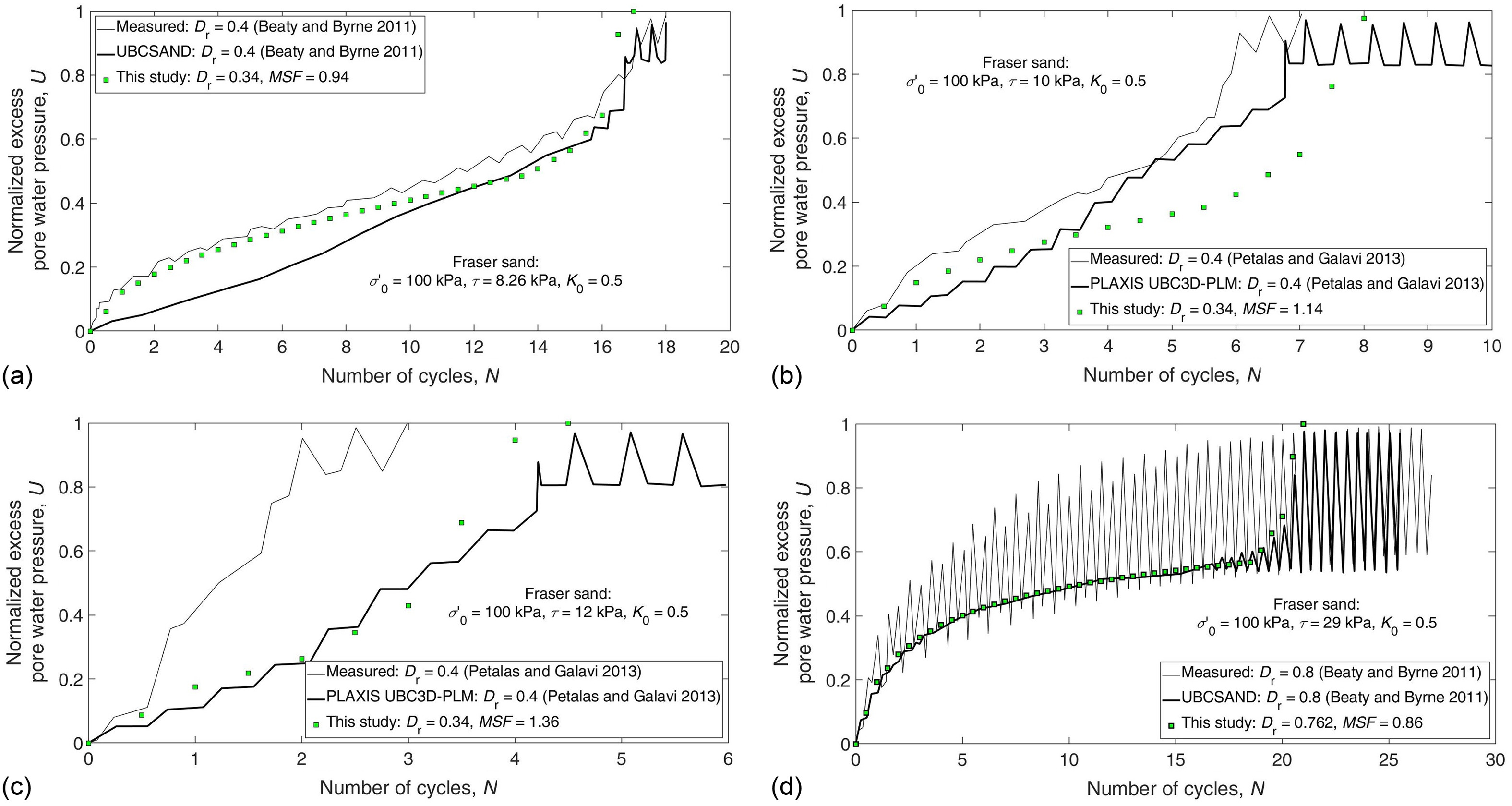
The discrepancies between the measured and predicted data in Fig. 23 were caused mainly by the difference of the cyclic resistance of the clean sand and Fraser sand. Although the main objective of this research was to calibrate the pore pressure model based on clean sand, it may be necessary to obtain different sets of calibration factors for other soils, because the

{CRR}_{7.5}

and

N_{liq}

of each soil may vary from one another and depending on the test method. Specifically, the

{CRR}_{7.5}

and

{CF}_{7.5}

are very significant in the calibration of the pore pressure model because they define the liquefaction resistance of a soil, and control CFratio. The

MSF - N_{liq}

relationship in Fig. 15 was biased toward clean sand because data were taken from Seed and Idriss (1982) and Boulanger and Ziotopoulou (2017). In addition, the

{CRR}_{7.5}

for Fraser sand at

D_{r} = 0.40

was observed to be different in comparison with the

{CRR}_{7.5}

proposed by Youd et al. (2001) and Idriss and Boulanger (2004) for clean sand. Based on Figs. 23(a–c), the

{CRR}_{7.5}

for Fraser sand at

D_{r} = 0.40

would be 0.0857. The

{CRR}_{7.5}

for clean sand at

D_{r} = 0.40

when

(N_{1})_{60} = 7.36

is 0.0906 and 0.1 based on the relationship given by Youd et al. (2001) and Idriss and Boulanger (2004), respectively. For

{CRR}_{7.5} = 0.1

, the MSF when

D_{r} = 0.40

,

σ_{0}^{'} = 100 kPa

, and

τ = 12.0 kPa

would be 1.20. The number of cycles to complete liquefaction

(N_{liq})

would be estimated to be 8.0 for

MSF = 1.20

using Eq. (25), whereas in the measured data shown in Fig. 23(c) for Fraser sand, the number of cycles to complete liquefaction was about 3.0. The simulation by Beaty and Byrne (2011) for Fraser sand used

(N_{1})_{60} = 6.9

instead of 7.36 for

D_{r} = 0.4

. Hence, they obtained

{CRR}_{7.5} = 0.0865

, which is closer to that of the

{CRR}_{7.5}

for Fraser sand. In the pore pressure model, the relative density had to be reduced so that the

{CRR}_{7.5}

would be closer to that of Fraser sand. In all cases in Fig. 23, the calibrated pore pressure model was able to predict a pore pressure rise almost similar to those of UBCSAND and PLAXIS UBC3D-PLM. Despite using different relative densities as an input parameter for the calibrated pore pressure model, the value of

D_{r}

utilized by the model still was in the range 5%–15% of the actual relative density, and the pore pressure rise of Fraser sand in the DSS still was represented fairly by the calibrated pore pressure model.

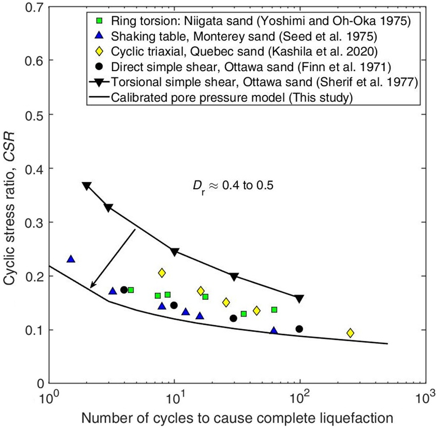
The behavior of various soils in different test devices for

D_{r} = 0.4

to 0.5 is shown in Fig. 24. Taking

D_{r} = 0.45

as an input parameter, the predicted CSR versus

N_{liq}

curve based on the calibrated pore pressure model was nearer to the experimental data from the direct simple shear test for Ottawa sand (Finn et al. 1971), the ring torsion test for Niigata sand (Yoshimi and Oh-Oka 1975), and the shaking table test for Monterey sand (Seed et al. 1975). If the original pore pressure model was not calibrated, the predicted curve would be similar to that of the experimental results of the Ottawa sand in the torsional simple shear device (Sherif et al. 1977), and close to that of the experimental results of the Quebec sand in the cyclic triaxial device (Kashila et al. 2020). The CSR curve predicted by the calibrated pore pressure model was close to that of Ottawa sand in the direct simple shear test (Fig. 24).

Fig. 24. Behavior of various soils in different test devices for $D_{r} = 0.4 - 0.5$ .

Practical Application of the Pore Pressure Model

The liquefaction potential evaluation of the soil is one the main applications of the calibrated pore pressure model. To evaluate the liquefaction potential of a soil at a certain density, initial effective stress, and earthquake magnitude (

M_{w}

) using the calibrated pore pressure model, the following steps should be followed:

1.

utilize a reliable relationship between

M_{w}

and MSF from the literature to obtain the magnitude scaling factor of the earthquake;

2.

determine the equivalent number of cycles to complete liquefaction

(N_{liq})

using Eq. (25) based on the MSF;

3.

determine the overall calibration factor CF using Eqs. (19), (23), (27), and (32) based on the parameters

D_{r}

,

σ_{0}^{'}

, and

N_{liq}

;

4.

determine parameters

{CF}_{crit}

and

α_{crit}

based on

D_{r}

;

5.

determine

(τ / σ_{0}^{'})_{crit}

based on

D_{r}

,

ϕ_{cv}

,

ξ_{r}

, and

n^{b}

;

6.

after obtaining the above parameters, apply Eqs. (12)–(15) to predict the pore pressure rise of the soil at any cyclic shear loading; and

7.

determine the cyclic shear loading that can cause complete liquefaction at

N_{liq}

as the CRR.

Limitations of the Pore Pressure Model

The calibrated pore pressure model presented in this study produced excellent results predicting the liquefaction resistance based on clean sand. However, the model has some limitations, and requires additional aspects to be considered in order to replicate closely the actual behavior of various soils. Basically, the original model was developed based on the behavior of Ottawa sand in the torsional simple shear device. However, the original model clearly was biased regarding the behavior of the soil in the device. To remove such bias and to consider various factors that affect liquefaction resistance, calibration of the original pore pressure model to that of clean sand was necessary. Hypothetically, if Ottawa sand was tested in another device, the original model constants such as

C 1

,

C 2

,

C 3

, and

α

may have been different from those originally obtained by Sherif et al. (1978). The shape of the liquefaction resistance curve for

N_{liq} = 15

and

σ'_{0} = 100 kPa

also may have been different from that initially obtained in Fig. 1 for Ottawa sand. Varying behaviors of pore pressure rise also are to be expected from different soils in various test devices.

It is possible to derive new sets of values of

C 1

,

C 2

,

C 3

,

α

, and other parameters such as

{CF}_{crit}

,

α_{crit}

, and

(τ / σ_{0}^{'})_{crit}

for other soils. However, extensive testing of the soil at various densities and cyclic shear loading is required to derive such parameters. It also is feasible to derive the necessary parameters of the original pore pressure model using well-known constitutive models and their calibrated constants for various soils. However, these constitutive models usually are only available in commercial finite-element programs, which sometimes are costly. Nonetheless, the determination of constants

C 1

,

C 2

, and

C 3

of the original model was based directly on the behavior of a soil in a specific device and its test procedures. This is the main reason why constitutive models have been proposed and recommended by many. Constitutive models can analyze the stress–strain response of a soil while simultaneously evaluating the pore pressure changes based on volume change. To predict the liquefaction resistance of another soil using the pore pressure model, it is more practical to introduce new calibration factors based on the behavior of the tested soil. One solution is to incorporate a calibration factor that considers the effect of fines content, which then widens the application of the current pore pressure model to silty soils.

Another limitation of the pore pressure model is its reliance on the complete liquefaction criterion. Beaty and Byrne (2011) assumed that liquefaction occurs when the normalized total excess pore-water pressure (

U

) exceeds 0.85 or when the maximum shear strain exceeds 3%. Because the current pore pressure model cannot evaluate the shear strains and is only stress-based, the complete liquefaction criterion was used to represent the manifestation of liquefaction. However, soils experiencing static bias may never reach a condition wherein the effective stress nearly equals the excess pore-water pressure despite having behavior that is consistent with liquefaction, such as when the shear strains exceed 3%. Beaty and Byrne (2011) mainly used the stress-based criterion of

U = 0.85

for soils with low densities, whereas the shear strain criterion of 3% often was satisfied for denser soils and for those with static bias. Data analyzed in this study did not involve static bias, and hence the model gave favorable results. Calibration of the model with static bias can be done by simplifying the model to achieve complete liquefaction. However, this may not fairly represent the actual behavior of the soil in the field and in laboratory tests. The use of a limiting

U

may have to be incorporated in the model if necessary. In addition, because strains are not considered in the current model, the contractive and dilative behavior, including fluctuations of the pore pressure during cyclic shear loading, cannot be modeled.

Conclusions

A method of adjusting the incremental pore pressure rise by use of calibration factors is introduced so that the pore pressure model can be calibrated based on the effect of the peak stress ratio, earthquake magnitude, and initial stress levels. In this study, the complete liquefaction criterion, defined as a state wherein the excess pore water pressure equals the initial effective stress, was used in the calibration. The shape of the excess pore-water pressure curve was considered by incorporating the critical stress ratio concept. The critical stress ratio concept allows for the consideration of the sudden rise in pore pressure at a certain stress ratio. At that certain stress ratio,

{CF}_{crit}

was suggested to take values greater than 1.0, and

α

was suggested to increase to 2.83 times its initial value such that the transition from the constant rate of pore pressure rise to the sudden pore pressure rise agrees well with the behavior of clean sand in direct simple shear tests. The critical stress ratio

(τ / σ^{'})_{crit}

was related to the peak stress ratio

(τ / σ^{'})_{peak}

to easily obtain the

(τ / σ^{'})_{crit}

at any density, and to allow for the consideration of the effect of the constant friction angle

ϕ_{c v}

.

After accounting for the shape effects of the pore pressure rise during cyclic loading of clean sand, the pore pressure model was calibrated based on the clean-sand base curve using a rational function, and by setting the initial effective stress to 100 kPa and the number of cycles to 15. To consider the effect of earthquake magnitude, a relationship between the magnitude scaling factor and the number of cycles to liquefaction

(N_{liq})

is proposed. Sets of CRR curves based on MSF were obtained, and their corresponding

N_{liq}

was used to obtain

{CFratio}_{N liq}

. The cyclic strength curves based on the initial effective stress were then adjusted using

K_{σ}

values proposed in the literature, enabling

{CFratio}_{σ^{'}}

to be obtained.

After the calibration factors were determined, the calibrated pore pressure model was verified by comparing data presented in the literature for clean sand and Fraser sand in direct simple shear tests, which showed that the model adequately predicted the behavior of the soils in the DSS. Calibration of the pore pressure model considering the effects of fines content,

K_{0}

, and static bias, as well as validation of the calibrated pore pressure model under earthquake loading, will be presented in a future study.

Notation

The following symbols are used in this paper:

$a_{N liq}$: constant that determines ${CFratio}_{N liq}$ ;
$a_{σ^{'}}$: constant that determines ${CFratio}_{σ^{'}}$ ;
$b_{N liq}$: constant that determines ${CFratio}_{N liq}$ ;
$b_{σ^{'}}$: constant that determines ${CFratio}_{σ^{'}}$ ;
$C 1$: constant in Eq. (4);
$C 2$: constant in Eq. (4);
$C 3$: constant in Eq. (4);
$CF$: overall calibration factor;
${CF}_{crit}$: additional calibration factor applied when ( $τ_{N} / σ_{N - 1}^{'}$ ) is greater than or equal to the critical stress ratio;
${CF}_{σ^{'}}$: calibration factor for initial effective stress;
${CF}_{7.5}$: calibration factor for magnitude 7.5 earthquake;
CFratio: ratio of overall CF to ${CF}_{7.5}$ ;
${CFratio}_{N liq}$: calibration factor ratio for earthquake magnitude or number of cycles to liquefaction;
${CFratio}_{σ^{'}}$: calibration factor ratio for initial effective stress;
${CRR}_{Mw}$: cyclic resistance ratio at certain earthquake magnitude;
${CRR}_{σ^{'}}$: cyclic resistance considering the influence of overburden effective stress;
${CRR}_{7.5}$: cyclic resistance ratio of clean sand for magnitude 7.5 earthquake;
$c_{N liq}$: constant that determines ${CFratio}_{N liq}$ ;
$c_{σ^{'}}$: constant that determines ${CFratio}_{σ^{'}}$ ;
$D_{r}$: relative density;
$K_{σ}$: overburden correction factor;
$K_{0}$: coefficient of earth pressure at rest;
$M_{w}$: moment magnitude;
$N$: current stress cycle;
$\bar{N}$: constant multiplier in Eq. (3), which characterizes the effect of the number of stress cycles;
$N_{eq}$: equivalent number of cycles;
$N_{eq, n}$: negative equivalent number of cycles;
$N_{eq, p}$: positive equivalent number of cycles;
$N_{liq}$: number of cycles to liquefaction;
$(N_{1})_{60}$: corrected standard penetration test blow count considering field procedures and overburden pressure;
$n^{b}$: parameter determining the value of the peak stress ratio;
$U$: normalized total excess pore-water pressure;
$u$: total excess pore-water pressure;
$α$: power of stress ratio ( $τ_{N} / σ_{N - 1}^{'}$ ) in Eq. (3);
$α_{crit}$: $α_{i} \times 2.83$ ;
$α_{i}$: initial value of $α$ ;
$Δ U$: normalized incremental excess pore water pressure;
$Δ U_{N, calib}$: calibrated normalized incremental excess pore pressure rise during the $N$ th cycle;
$Δ U_{N, n}$: normalized incremental excess pore pressure rise due to negative cyclic shear stress $τ_{N, n}$ during the $N$ th cycle;
$Δ U_{N, p}$: normalized incremental excess pore pressure rise due to positive cyclic shear stress $τ_{N, p}$ during $N$ th cycle;
$Δ u$: incremental excess pore water pressure rise;
$ξ_{r}$: relative state parameter index;
$σ^{'}$: effective pressure;
$σ_{0}^{'}$: initial effective pressure;
$τ$: shear stress;
$(τ / σ^{'})_{crit}$: critical stress ratio;
$(τ / σ^{'})_{peak}$: peak stress ratio;
$τ_{N, n}$: negative cyclic shear stress during $N$ th cycle;
$τ_{N, p}$: positive cyclic shear stress during $N$ th cycle;
$ϕ_{c v}$: constant friction angle; and
$ϕ_{peak}$: peak friction angle.

Data Availability Statement

Some or all data, models, or code that support the findings of this study are available from the corresponding author upon reasonable request.

Acknowledgments

This research was supported by the Basic Science Research Program through the National Research Foundation of Korea (NRF) funded by the Ministry of Education (NRF-2021R1A6A1A0304518511 and NRF-2020R1I1A3A04036506).

References

Andrus, R. D., and K. H. Stokoe. 1997. “Liquefaction resistance based on shear wave velocity.” In Proc., NCEER Workshop on Evaluation of Liquefaction Resistance of Soils, 89–128. Bufallo, NY: National Center for Earthquake Engineering Research.

Google Scholar

Beaty, M. H., and P. M. Byrne. 2011. “UBCSAND constitutive model version 904aR.” Accessed February 1, 2011. https://bouassidageotechnics.files.wordpress.com/2016/12/ubcsand_udm_documentation.pdf.

Google Scholar

Boulanger, R. W. 2003. “High overburden stress effects in liquefaction analyses.” J. Geotech. Geoenviron. Eng. 129 (12): 1071–1082. https://doi.org/10.1061/(ASCE)1090-0241(2003)129:12(1071).

Google Scholar

Boulanger, R. W., and I. M. Idriss. 2004. “State normalization of penetration resistances and the effect of overburden stress on liquefaction resistance.” In Vol. 2 of Proc., 11th Int. Conf. on Soil Dynamics and Earthquake Engineering, and 3rd Int. Conf. on Earthquake Geotechnical Engineering, 484–491. Singapore: Stallion Press.

Google Scholar

Boulanger, R. W., and K. Ziotopoulou. 2017. PM4Sand (version 3.1): A sand plasticity model for earthquake engineering applications. Davis, CA: Center for Geotechnical Modeling, Dept. of Civil and Environmental Engineering, Univ. of California.

Google Scholar

Castro, G. 1969. “Liquefaction of sands.” Ph.D. thesis, Dept. of Engineering and Applied Physics, Harvard Univ.

Google Scholar

Cetin, K. O., R. B. Seed, A. Der Kiureghian, K. Tokimatsu, L. F. Harder Jr., R. E. Kayen, and R. E. S. Moss. 2004. “Standard penetration test-based probabilistic and deterministic assessment of seismic soil liquefaction potential.” J. Geotech. Geoenviron. Eng. 130 (12): 1314–1340. https://doi.org/10.1061/(ASCE)1090-0241(2004)130:12(1314).

Google Scholar

Elgamal, A. W., R. Dobry, E. Parra, and Z. Yang. 1998. “Soil dilation and shear deformations during liquefaction.” In Proc., 4th Int. Conf. on Case Histories in Geotechnical Engineering, 1238–1259. Rolla, MO: Missouri Univ. of Science and Technology.

Google Scholar

Finn, W. D. L., J. J. Emery, and Y. P. Gupta. 1970. “A shaking table study of the liquefaction of saturated sands during earthquakes.” In Proc., 3rd European Symp. on Earthquake Engineering, 253–262. Sofia, Bulgaria: Bulgarian Academy of Sciences.

Google Scholar

Finn, W. D. L., D. J. Pickering, and P. L. Bransby. 1971. “Sand liquefaction in triaxial and simple shear tests.” J. Soil Mech. Found. Div. 97 (4): 639–659. https://doi.org/10.1061/JSFEAQ.0001579.

Google Scholar

Harder, L. F., and R. W. Boulanger. 1997. “Application of K_σ and K_α correction factors.” In Proc., NCEER Workshop on Evaluation of Liquefaction Resistance of Soils, edited by T. L. Youd and I. M. Idriss, 167–190. Buffalo, NY: National Center for Earthquake Engineering Research.

Google Scholar

Hynes, M. E., and R. Olsen. 1998. “Influence of confining stress on liquefaction resistance.” In Proc., Int. Symp. on the Physics and Mechanics of Liquefaction, 145–152. Rotterdam, Netherlands: Balkema.

Google Scholar

Idriss, I. M., and R. W. Boulanger. 2004. “Semi-empirical procedures for evaluating liquefaction potential during earthquakes.” In Vol. 1 of Proc., 11th Int. Conf. on Soil Dynamics and Earthquake Engineering, and 3rd Int. Conf. on Earthquake Geotechnical Engineering, 32–56. Singapore: Stallion Press.

Google Scholar

Idriss, I. M., and R. W. Boulanger. 2008. Soil liquefaction during earthquakes. Oakland, CA: Earthquake Engineering Research Institute.

Google Scholar

Ishibashi, I., M. A. Sherif, and C. Tsuchiya. 1977. “Pore-pressure rise mechanism and soil liquefaction.” Soils Found. 17 (2): 17–27. https://doi.org/10.3208/sandf1972.17.2_17.

Google Scholar

Ishihara, K., and S.-I. Li. 1972. “Liquefaction of saturated sand in triaxial torsion shear test.” Soils Found. 12 (2): 19–39. https://doi.org/10.3208/sandf1972.12.19.

Google Scholar

Kashila, M., M. N. Hussein, M. Karray, and M. Chekired. 2020. “Liquefaction resistance from cyclic simple and triaxial shearing: A comparative study.” Acta Geotech. 16 (Jun): 1735–1753. https://doi.org/10.1007/s11440-020-01104-6.

Google Scholar

Konstadinou, M., and V. N. Georgiannou. 2014. “Prediction of pore water pressure generation leading to liquefaction under torsional cyclic loading.” Soils Found. 54 (5): 993–1005. https://doi.org/10.1016/j.sandf.2014.09.010.

Google Scholar

Ladd, R. S., and M. L. Silver. 1975. “Discussion of ‘Soil liquefaction by torsional simple shear device’.” J. Geotech. Eng. Div. 101 (8): 827–829. https://doi.org/10.1061/AJGEB6.0001427.

Google Scholar

Petalas, A., and V. Galavi. 2013. “Plaxis liquefaction model UBC3D-PLM.” Accessed June 7, 2013. https://communities.bentley.com/cfs-file/__key/communityserver-wikis-components-files/00-00-00-05-58/UBC3D_2D00_PLM_2D00_REPORT.June2013.pdf.

Google Scholar

Seed, H. B. 1981. “Earthquake-resistant design of earth dams.” In Proc., First Int. Conf. on Recent Advances in Geotechnical Earthquake Engineering and Soil Dynamics, 1157–1173. Rolla, MO: Missouri Univ. of Science and Technology.

Google Scholar

Seed, H. B., I. Arango, and C. K. Chan. 1975. Evaluation of soil liquefaction potential for level ground during earthquakes: A summary report. Seattle: Shannon and Wilson. https://doi.org/10.2172/7146067.

Google Scholar

Seed, H. B., and I. M. Idriss. 1982. Ground motions and soil liquefaction during earthquakes, 134. Oakland, CA: Earthquake Engineering Research Institute.

Google Scholar

Seed, H. B., and W. H. Peacock. 1971. “Test procedures for measuring soil liquefaction characteristics.” J. Soil Mech. Found. Div. 97 (8): 1099–1119. https://doi.org/10.1061/JSFEAQ.0001649.

Google Scholar

Seed, H. B., K. Tokimatsu, L. F. Harder, and R. M. Chung. 1985. “Influence of SPT procedures in soil liquefaction resistance evaluations.” J. Geotech. Eng. 111 (12): 1425–1445. https://doi.org/10.1061/(ASCE)0733-9410(1985)111:12(1425).

Google Scholar

Sherif, M. A., I. Ishibashi, and C. Tsuchiya. 1978. “Pore-pressure prediction during earthquake loadings.” Soils Found. 18 (4): 19–30. https://doi.org/10.3208/sandf1972.18.4_19.

Google Scholar

Sherif, M. A., C. Tsuchiya, and I. Ishibashi. 1977. Pore pressure rise of saturated sands during cyclic loading. Washington, DC: Univ. of Washington.

Google Scholar

Wei, J. 2021. “DEM exploration of confining stress effect in cyclic liquefaction of granular soils.” Comput. Geotech. 136 (Aug): 104214. https://doi.org/10.1016/j.compgeo.2021.104214.

Google Scholar

Yang, M., M. Taiebat, and F. Radjaï. 2022. “Liquefaction of granular materials in constant-volume cyclic shearing: Transition between solid-like and fluid-like states.” Comput. Geotech. 148 (Aug): 104800. https://doi.org/10.1016/j.compgeo.2022.104800.

Google Scholar

Yoshimi, Y., and H. Oh-Oka. 1975. “A ring torsion apparatus for simple shear tests.” In Proc., 8th Int. Conf. on Soil Mechanics and Foundation Engineering, 501–506. London: International Society for Soil Mechanics and Geotechnical Engineering.

Google Scholar

Youd, T. L., et al. 2001. “Liquefaction resistance of soils: Summary report from the 1996 NCEER and

1998 NCEER / NSF

workshops on evaluation of liquefaction resistance of soils.” J. Geotech. Geoenviron. Eng. 127 (10): 817–833. https://doi.org/10.1061/(ASCE)1090-0241(2001)127:10(817).

Google Scholar

Yu, J.-K., R. Wang, and J.-M. Zhang. 2022. “Importance of liquefaction resistance and fabric anisotropy simulation capability of constitutive models for liquefiable ground seismic response analysis.” Comput. Geotech. 150 (Oct): 104928. https://doi.org/10.1016/j.compgeo.2022.104928.

Google Scholar

Information & Authors

Information

Published In

Journal of Geotechnical and Geoenvironmental Engineering

Volume 149 • Issue 8 • August 2023

Copyright

This work is made available under the terms of the Creative Commons Attribution 4.0 International license, https://creativecommons.org/licenses/by/4.0/.

History

Received: Oct 25, 2022

Accepted: Mar 20, 2023

Published online: May 27, 2023

Published in print: Aug 1, 2023

Discussion open until: Oct 27, 2023

Authors

Affiliations

Hyeong-Joo Kim, Ph.D., M.ASCE [email protected]

Professor, Dept. of Civil Engineering, Kunsan National Univ., Gunsan 54150, Republic of Korea. Email: [email protected]

View all articles by this author

Peter Rey Dinoy, Ph.D. https://orcid.org/0000-0002-5884-1748 [email protected]

Researcher, Dept. of Civil and Environmental Engineering, Renewable Energy Research Institute, Kunsan National Univ., Gunsan 54150, Republic of Korea (corresponding author). ORCID: https://orcid.org/0000-0002-5884-1748. Email: [email protected]

View all articles by this author

Hyeong-Soo Kim, Ph.D. [email protected]

Researcher, Dept. of Civil and Environmental Engineering, Kunsan National Univ., Gunsan 54150, Republic of Korea. Email: [email protected]

View all articles by this author

Tae-Woong Park, Ph.D. [email protected]

Research Professor, Renewable Energy Research Institute, Kunsan National Univ., Gunsan 54150, Republic of Korea. Email: [email protected]

View all articles by this author

Young-Soung Jeong [email protected]

P.E.

Engineer, Dept. of Civil and Environmental Engineering, Kunsan National Univ., Gunsan 54150, Republic of Korea. Email: [email protected]

View all articles by this author

Metrics & Citations

Metrics

Citations

Download citation

If you have the appropriate software installed, you can download article citation data to the citation manager of your choice. Simply select your manager software from the list below and click Download.

Abstract

Introduction

Formulation of Density-Based Pore Pressure Model

Relationship between Incremental Excess Pore Water Pressure, Shear Stress Ratio, and Number of Cycles

Prediction of Pore Pressure Rise under Earthquake Loading

Calibration of Density-Based Pore Pressure Model

Calibration of Pore Pressure Model Based on Behavior of Clean Sand in Direct Simple Shear Tests

Calibration Based on Triggering Liquefaction Curves

Calibration Based on Clean Sand Base Curve

Calibration Considering Magnitude Scaling Factor or Number of Cycles to Liquefaction

Calibration Considering Influence of Initial Effective Stress

Verification of Calibrated Pore Pressure Model

Practical Application of the Pore Pressure Model

Limitations of the Pore Pressure Model

Conclusions

Notation

Data Availability Statement

Acknowledgments

References

Information

Published In

Copyright

History

ASCE Technical Topics:

Authors

Affiliations

Metrics

Citations

Download citation

Figures

Other

Share

Copy the content Link

Share with email

Share

Request Username

Create a new account

Change Password

Password Changed Successfully

Verify Phone

Congrats!