Shallow Seafloor Sediments: Density and Shear Wave Velocity

Salva Ramirez, Marisol; Park, Junghee; Terzariol, Marco; Jiang, Jiming; Santamarina, J. Carlos

doi:10.1061/JGGEFK.GTENG-10759

Open access

Technical Papers

Feb 28, 2023

Shallow Seafloor Sediments: Density and Shear Wave Velocity

Authors: Marisol Salva Ramirez https://orcid.org/0000-0002-0169-0918, Junghee Park https://orcid.org/0000-0001-7033-4653 [email protected], Marco Terzariol https://orcid.org/0000-0001-5362-1968, Jiming Jiang, and J. Carlos Santamarina, A.M.ASCE https://orcid.org/0000-0001-8708-2827Author Affiliations

Publication: Journal of Geotechnical and Geoenvironmental Engineering

Volume 149, Issue 5

https://doi.org/10.1061/JGGEFK.GTENG-10759

PDF

Abstract

Near-surface seafloor properties affect offshore mining and infrastructure engineering. Shallow seafloor sediments experience extremely low effective stress, and consequently, these sediments exhibit very low in-situ density, shear wave velocity, and shear stiffness. We combined data extracted from the literature with new laboratory and field results to develop a comprehensive understanding of shallow seafloor sediments. First, we explored the sediment-dependent self-compaction characteristics starting with the asymptotic void ratio at the interface between the water column and the sediment column. The asymptotic void ratio depends on the particle size and shape in coarse-grained sediments and on mineralogy and pore fluid chemistry in fine-grained clayey sediments; overall, the asymptotic void ratio correlates with the sediment-specific surface and compressibility. Second, we developed a fork-type insertion probe to measure shear wave velocity profiles with depth. Detailed data analyses confirm the prevalent role of effective stress on shear wave velocity

V_{s} = α (σ_{m}^{'} / kPa)^{β}

, and the inverse relationship between

α

and

β

parameters reveals that electrical interactions alter the velocity profile only in very high specific surface area sediments at very low effective stress and shows that ray bending affects the computed velocities only in the upper few centimeters (for the probe geometry used in this study). Probe insertion causes excess pore fluid pressure and effective stress changes; the ensuing time-dependent diffusion detected through shear wave velocity changes can be analyzed to estimate the coefficient of consolidation. Shear wave velocity profiles and velocity transients after insertion provide valuable information for sediment preclassification and engineering design.

Introduction

Near-surface seafloor properties affect the design, serviceability, safety, and long-term performance of seafloor geosystems such as oil and gas pipelines, transmission lines, anchors, caissons and skirted foundations, mudmats, and deep-sea mining operations (Andersen et al. 2008; Randolph 2012; Feng et al. 2014; Tom and White 2019). Shallow seafloor sediments experience extremely low effective stress; therefore, in the absence of diagenesis, the in-situ density

ρ

and shear wave velocity

V_{s}

are very low as well.

Sampling alters the sediment stress history and fabric. Furthermore, typical piston cores may puncture through and bypass shallow fine-grained sediments. Consequently, sample-based densities and shear wave velocities may not necessarily represent the in-situ sediment stiffness of shallow sediments (see data in Dai and Santamarina 2014). On the other hand, S-wave velocity measurements in the field are cumbersome and may require scuba divers or remotely operated vehicles ROVs (Hamilton et al. 1970; Richardson et al. 1991; Wang et al. 2018).

This study aims to provide insights into sediment density and shear stiffness under very low effective stress near the sediment-water interface. First, we measure densities for a wide range of soil types using sedimentation tests and various pore fluids. Then, we determine S-wave velocity versus depth profiles in laboratory specimens and natural sediments in the field using a high-sensitivity probe built for this study. In both cases, we complement our measurements with extensive datasets compiled from the literature.

In-Situ Density—Asymptotic Void Ratio

How loose can a granular medium be when it becomes a sediment? What is its density sediment-water interface where the effective stress vanishes

σ_{z}^{'} \to 0 ?

The answer to these questions establishes the boundary between the water column and the sediment column, the origin of self-compaction trends, the beginning of shear wave propagation and shear strength, and the impedance mismatch that defines bathymetric measurements. Given its relevance to shallow seafloor sediments, we investigate the sediment-water boundary first.

A sediment attains a characteristic density

ρ_{o}

when particles start forming a granular skeleton at the sediment-water interface. The characteristic density corresponds to the asymptotic void ratio

e_{L}

as the effective stress

σ_{z}^{'} \to 0

ρ_{o} = ρ_{w} \frac{G_{s} + e_{L}}{1 + e_{L}}

(1)

where

ρ_{w}

= water mass density; and

G_{s}

= mineral-specific gravity. Interparticle contact and jamming are geometrically defined in the case of coarse grains (Liu and Nagel 1998; Radjai et al. 1999; O’Hern et al. 2001). However, the slurry-to-sediment transition is gradual in fine-grained sediments where particles experience long-range electrical interaction. Therefore, in this study, we analyze coarse and fine-grained sediments separately to discern the effects of particle size, shape, mineralogy, and pore fluid chemistry on the asymptotic void ratio using new experimental data and published results.

Coarse-Grained Sediments—Gravels, Sands, and Silts

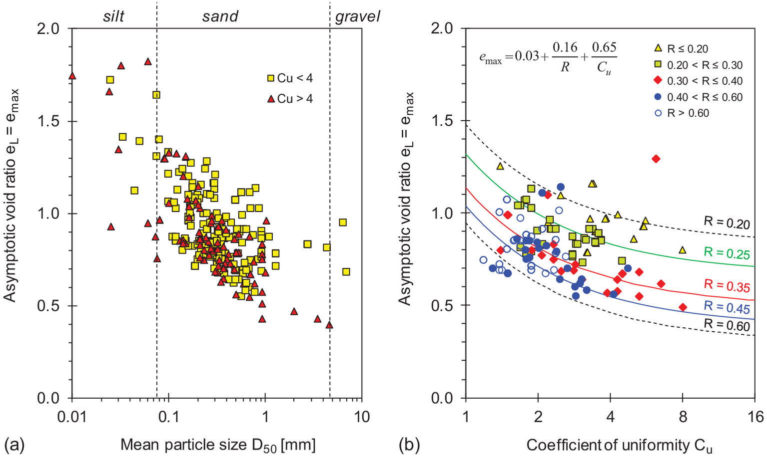
Coarse grains respond to gravimetric and skeletal forces within kinematic constraints. Let us consider the maximum void ratio

e_{\max}

as the asymptotic void ratio

e_{L}

a coarse-grained sediment may reach at low effective stress

σ_{z}^{'} \to 0

[Note:

e_{\max}

is a procedurally-defined parameter, as per ASTM D4254 (ASTM 2006)]. Fig. 1 shows data compiled for gravels, sands, and silts. The asymptotic void ratio

e_{L} \approx e_{\max}

decreases as the mean particle size

d_{50}

increases [Fig. 1(a)] and as the coefficient of uniformity

C_{u}

and roundness

R

increase [Fig. 1(b)]. The model fitted to the data in Fig. 1(b) captures the role of uniformity

C_{u}

and roundness

R

(modified after Youd 1973; Cho et al. 2006)

e_{L} = e_{\max} = 0.03 + \frac{0.16}{R} + \frac{0.65}{C_{u}}

(2)

Fig. 1. Coarse-grained sediments: asymptotic void ratio $e_{L} = e_{\max}$ for gravels, sands, and silts: (a) asymptotic void ratio $e_{L}$ versus mean particle size $D_{50}$ ; and (b) asymptotic void ratio $e_{L}$ versus coefficient of uniformity $C_{u}$ and roundness $R$ . (Data from Youd 1973; Mayne and Kulhawy 1982; Been and Jefferies 1985; Ishihara 1993; Evans and Zhou 1995; Terzaghi et al. 1996; Burland et al. 1996; Sukumaran and Ashmawy 2001; Thevanayagam et al. 2002; Hight et al. 2003; Chin et al. 2006; Cho et al. 2006; Cerato and Lutenegger 2006; Simoni and Houlsby 2006; Yang et al. 2006; Murthy et al. 2007; Carraro et al. 2009; Chong and Santamarina 2016; Altuhafi et al. 2016; Hryciw et al. 2016.)

Fine-Grained Sediments—Clays

Mineralogy and pore fluid chemistry affect the interaction between small clay-sized grains. We used sedimentation tests to assess the loosest fabric kaolinite and bentonite can attain in various pore fluids (Note: the test protocol is based on flat bottom tubes and low mass fraction suspensions—details in Palomino and Santamarina 2005). In addition, we compiled published sedimentation test data.

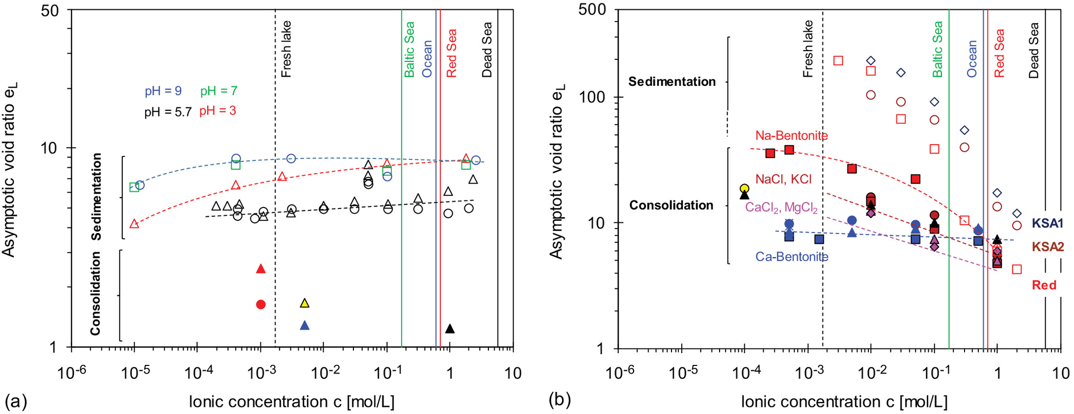
Figs. 2(a and b) shows the asymptotic void ratio

e_{L}

versus ionic concentration for low- and high-plasticity clays. Reference vertical lines show the ionic concentration found in various water bodies, from freshwater lakes to oceans and brine pools. Data support the following observations:

•

Low- and high-plasticity clays exhibit distinct sensitivities to pore fluid chemistry (this confirms sensitivity studies in Jang and Santamarina 2016).

•

The asymptotic void ratio e_L for low plasticity kaolinite ranges from

e_{L} = 4

-to-9 [Fig. 2(a)] and is more sensitive to pH than to ionic concentration: clearly, fabric formation reflects pH-dependent edge and surface charges, i.e., face-to-face aggregation versus dispersed fabric.

•

The asymptotic void ratio e_L for high-plasticity bentonite is in the range of

e_{L} = 5

-to-40 [Fig. 2(b)]. In contrast to kaolinite, the asymptotic void ratio does depend on ionic strength, i.e., the concentration co and valance z of prevailing cations, in line with the diffused double layer thickness

{ϑ \propto (c_{o} \cdot z_{2})}_{- 1 / 2}

(Santamarina et al. 2001; Mitchell and Soga 2005).

Fig. 2. Fine-grained sediments: asymptotic void ratio $e_{L}$ for clays as a function of ionic concentration: (a) *low plasticity clays*—kaolinite RP2 (triangles) and SA1 (circles). Open symbols indicate asymptotic void ratio estimated from sedimentation test results: black open triangles and circles correspond to results conducted as part of this study, and the other colored open symbols correspond to the kaolinite RP2 sedimentation test results extracted from Palomino and Santamarina (2005). Filled symbols at low void ratios show values estimated by fitting consolidation data using Eq. (3): Red triangle and circle [data from Cha (2021); Yellow triangle from Fam and Santamarina 1997; blue and black triangles from Kang (2015)]; and (b) *high plasticity clays* - Bentonite. Open symbols indicate the asymptotic void ratio estimated from sedimentation test results conducted as part of this study. Filled symbols indicate asymptotic void ratio estimated from consolidation tests by using the consolidation model [Eq. (3)]. (Data from Mesri and Olson 1971; Studds et al. 1996, 1998.)

Asymptotic Void Ratio and Compressibility—Caution

The asymptotic void ratio

e_{L}

correlates with compressibility (Skempton 1970; Burland 1990). Therefore, we can anticipate that

e_{L}

and

ρ_{o}

are intimately related to self-compaction trends and the evolution of stiffness with depth. However, can consolidation tests be used to predict the asymptotic void ratio? We compiled consolidation data gathered for normally consolidated sediments and fitted trends using an asymptotically correct consolidation model to recover the void ratio

e_{L}

as

σ_{z}^{'} \to 0

(Bauer 1996; Gregory et al. 2006; reformulated in Chong and Santamarina 2016—see Supplemental Materials for

e_{L}

determination):

e_{z} = e_{H} + (e_{L} - e_{H}) \exp [- {(\frac{σ_{z}^{'}}{σ_{c}^{'}})}^{η}]

(3)

where

e_{z}

= void ratio at depth z and

e_{H}

is the void ratio at very high effective stress at

σ_{z}^{'} \to \infty

. When the applied effective stress reaches the characteristic stress

σ_{z}^{'} = σ_{c}^{'}

, the degree of consolidation is

(e_{z} + e_{H}) / (e_{L} - e_{H}) = 0.37

; hence, the soil has experienced 63% of the possible volume change (

e_{L} - e_{H}

) between the two asymptotic void ratios. The model parameter

η

reflects the void ratio sensitivity to changes in effective stress. Previous studies compiled depth-dependent and stress-dependent void ratio data for fine- to coarse-grained sediments and confirmed that a single value

η \approx 1 / 3

adequately fits all trends [examples: hydrate pore habits in Terzariol et al. (2020), microbial cell counts in deep sedimentary basins in Park and Santamarina (2020), and geoacoustic properties in Lyu et al. (2021)].

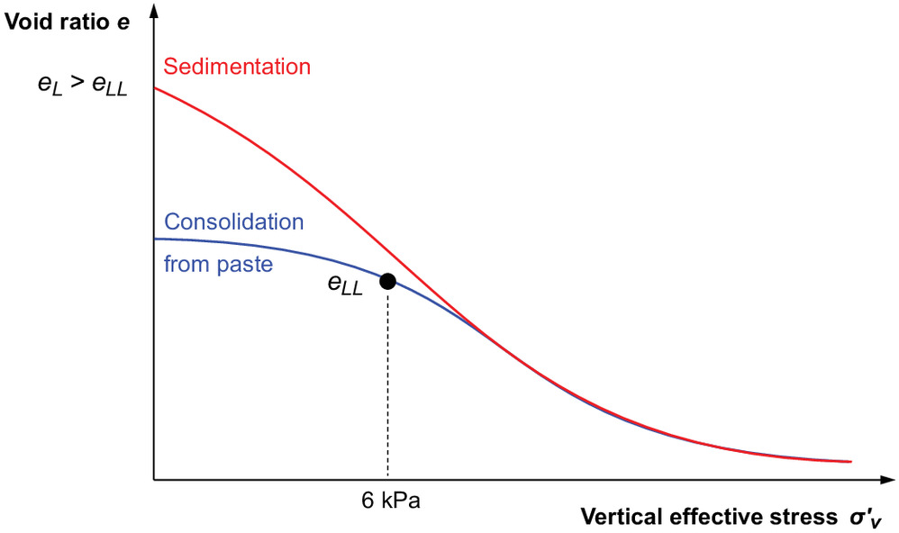
Results in Figs. 2(a and b) show that consolidation data underpredict the asymptotic void ratio for near-surface seafloor sediments even when tested specimens start as clay pastes prepared at a high water content, such as 1.1-to-1.5LL (Burland 1990). Schematic trends in Fig. 3 compare a clay response when consolidation starts from its true asymptotic void ratio

e_{L}

as

σ_{z}^{'} \to 0

and from a paste prepared at a water content

ω % > L L

. For reference, the liquid limit corresponds to

\sim 6 kPa

suction (Russell and Mickle 1970; Hong et al. 2010); conversely, the void ratio at 1 kPa effective stress correlates with the void ratio at the liquid limit as

e_{1 kPa} = 1.25 \cdot e_{LL}

(based on 28 datapoints with

R^{2} = 0.92

- Chong and Santamarina 2016). Clearly, suction preconsolidates pastes, and consequently, typical consolidation tests with remolded specimens underpredict the true asymptotic void ratio needed for seafloor sediment analyses (Fig. 3).

Fig. 3. Anticipated void ratio versus effective trends obtained from sedimentation and consolidation tests. Note: $e_{L L}$ is the void ratio at the liquid limit $L L$ .

Trends as a Function of the Specific Surface Area

The smallest grain dimension determines its specific surface area

S_{s} [m^{2} / g]

, i.e., the thickness of platy clay particles or the smallest diameter of ellipsoidal coarse grains. Let us explore the trend between the asymptotic void ratio

e_{L}

and specific surface area. When

S_{s}

values are not reported, we estimate the specific surface area from other available data. In the case of sands, we use the mean particle size

d_{50}

[mm] and the coefficient of uniformity

C_{u}

(Santamarina et al. 2002)

S_{s} = \frac{3 (C_{u} + 7)}{4 ρ_{w} G_{s} d_{50}} For sands

(4)

where

ρ_{w}

= water mass density; and

G_{s}

= mineral-specific gravity. In the case of fine-grained sediments, we estimate the specific surface area from the liquid limit

L L

(Farrar and Coleman 1967):

S_{s} = \frac{4}{3} (L L - 25) For clays and L L > 25

(5)

Fig. 4 summarizes the dataset compiled for this study; the mean trend is (Note: based on

n = 338

datapoints; for the least squares fit, error is defined in terms of the logarithm of the void ratio):

e_{L} = 0.9 + 0.03 \frac{S_{s}}{[m^{2} / g]}

(6)

Fig. 4. Asymptotic void ratio $e_{L}$ for coarse and fine-grained soils as a function of specific surface $S_{s}$ . Reference fabrics on the right: a 3D card-castle made of platelets with slenderness $a$ , and a simple cubic packing of monosized spheres. Note: 338 data points. (Data from Studds et al. 1996; Mesri and Olson 1971; Palomino and Santamarina 2005.)

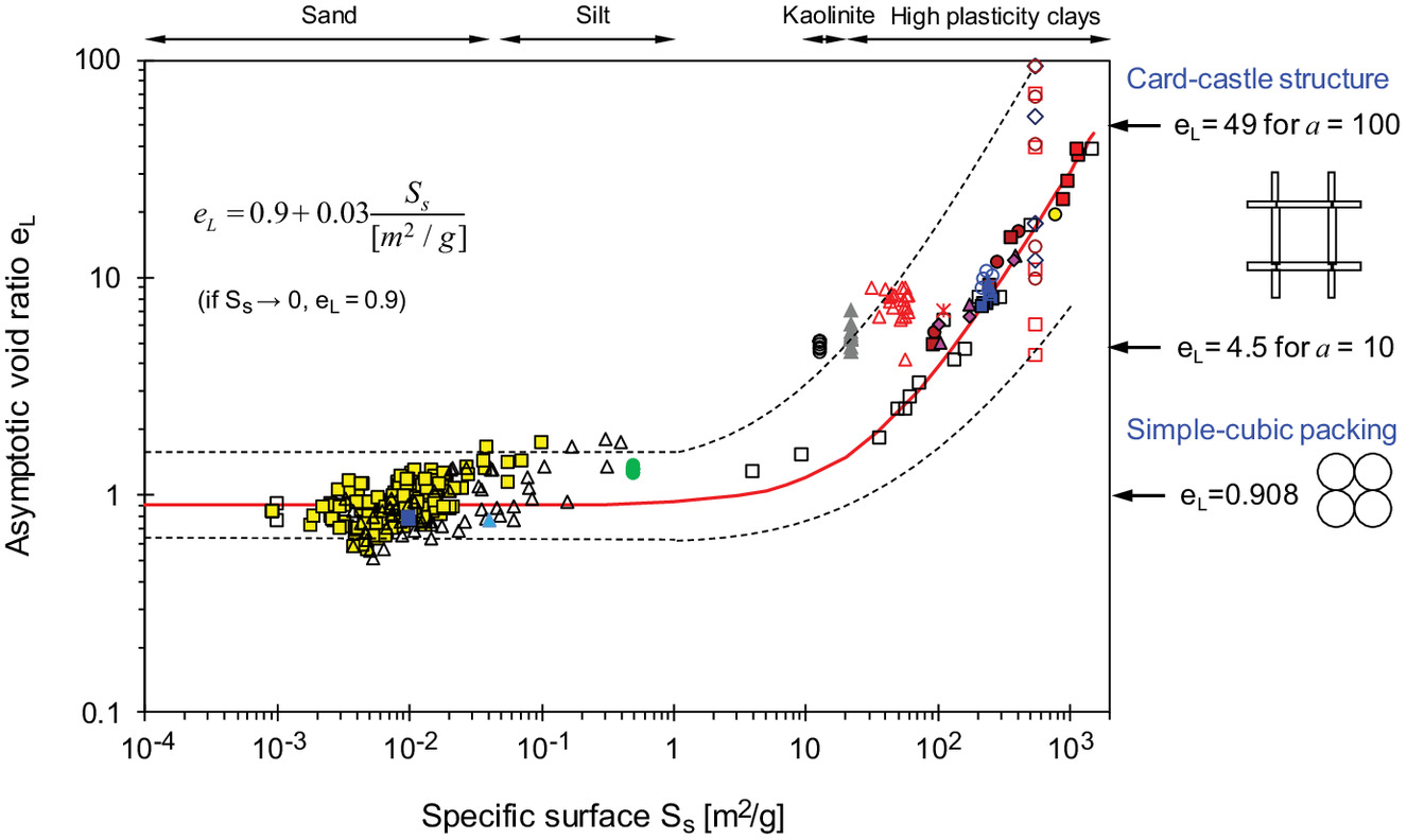
The maximum void ratio for the packing of mono-sized spherical particles corresponds to the simple cubic configuration

e_{L} = 0.908

; this is approximately the mean value of the maximum void ratio measured for loosely packed and poorly graded coarse-grained sediments. Variability in fine-grained soils reflects pore fluid effects; for reference, the void ratio for an open card-castle configuration is

e_{L} = (a - 2) / 3

, where

a = L_{p} / t_{p}

is the particle slenderness ratio defined by the particle length

L_{p}

and thickness

t_{p}

(see Supplemental Materials). Data in Fig. 4 show that these simple geometric models provide valuable physical insights into fabric conditions at the asymptotic void ratio.

Shear Wave Velocity

Small-strain shear waves propagate through granular media without causing fabric changes; therefore, shear wave velocity measurements are an assessment of state. From the theory of elasticity, the shear wave velocity

V_{s}^{2} = G_{\max} / ρ

is a function of the sediment small-strain shear modulus

G_{\max}

and density

ρ

. The following sections present a tool developed to measure the shear wave velocity in shallow seafloor sediments and an extensive database that combines new laboratory and field measurements together with data gathered from published studies.

S-Wave Velocity Probe

We designed and built a multiphysics probe for shallow seafloor sediment characterization (Fig. 5). This modular penetration-based instrument includes sensors to measure pressure, temperature, electrical conductivity, permittivity, pH, and 3D acceleration [Fig. 5(a)]. The probe is deployable in either a stand-alone mode or wired to the vessel (Terzariol 2015). The pressure-balanced tip allows for precise measurements of soft sediment strength regardless of the water depth (US Patent 17/604,853).

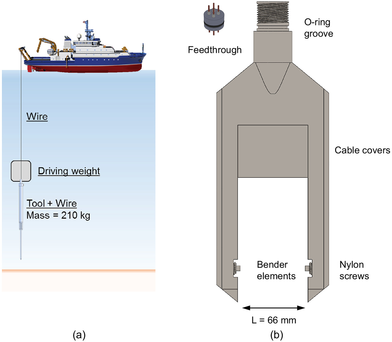
Fig. 5. Multiphysics insertion probe: (a) field deployment is either stand-alone battery-powered or wired to the vessel; and (b) design of fork-type field shear wave velocity probe.

The segment for shear wave measurements is mounted at the front of the multiphysics probe and uses bender elements as shear wave transducers [Fig. 5(b) - design based on Klein and Santamarina 2005; Yoon et al. 2008; Lee et al. 2009]. The open fork geometry avoids reflections from the lateral P-wave lobes generated by the bender elements. Bender elements are mounted in threaded plastic nylon screws to reduce wave transmission along the fork and to facilitate their replacement (parallel-type;

12.7 mm \times 8 mm \times 0.7 mm

; mounted with a 5 mm cantilevered length and 7.7 mm anchored length), and they are coated with silver paint and grounded to minimize electrical crosstalk (details in Lee and Santamarina 2005). The tip-to-tip distance between bender elements

L = 66 mm

is longer than the anticipated wavelengths.

A ceramic feedthrough connects the fork to the upper probe that houses the electronic controls [Fig. 5(b)]. The function generator sends a 10 V step signal every 50 ms to the source bender element. The filter amplifier connected to the receiving bender element applies a band-pass filter (500 Hz to 200 kHz).

Experimental Study: Laboratory and Field

We tested the probe in the laboratory using sediment beds prepared with kaolinite, silica flour, and fine sand housed within large-diameter plexiglass chambers (300 mm in diameter and 600 mm in height—inset in Fig. 6). The three beds were formed from diluted deaired slurries (initial water content

ω > 2,000 %

) and were allowed to settle until they reached a constant sediment height. Then, we measured S-wave velocities every 1-to-2 cm of probe penetration; to enhance the signal-to-noise ratio, we stacked 1,024 signals and stored the resulting signal. The probe penetration rate was

\sim 2 cm / s

. At selected insertion depths, we held the probe in place until the first arrival time reached a constant value, i.e., complete dissipation of excess pore-water pressure (details in the following section). Fig. 6 displays the cascade of shear wave signals gathered at different depths in the clay, silt, and sand sediments after pore fluid pressure dissipation. The time to first arrival decreases with depth in all sediments. Minor deviations from the general trend suggest internal layering.

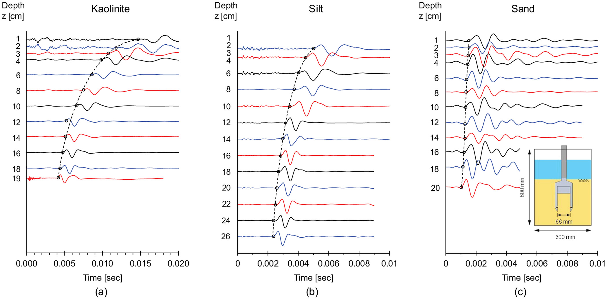
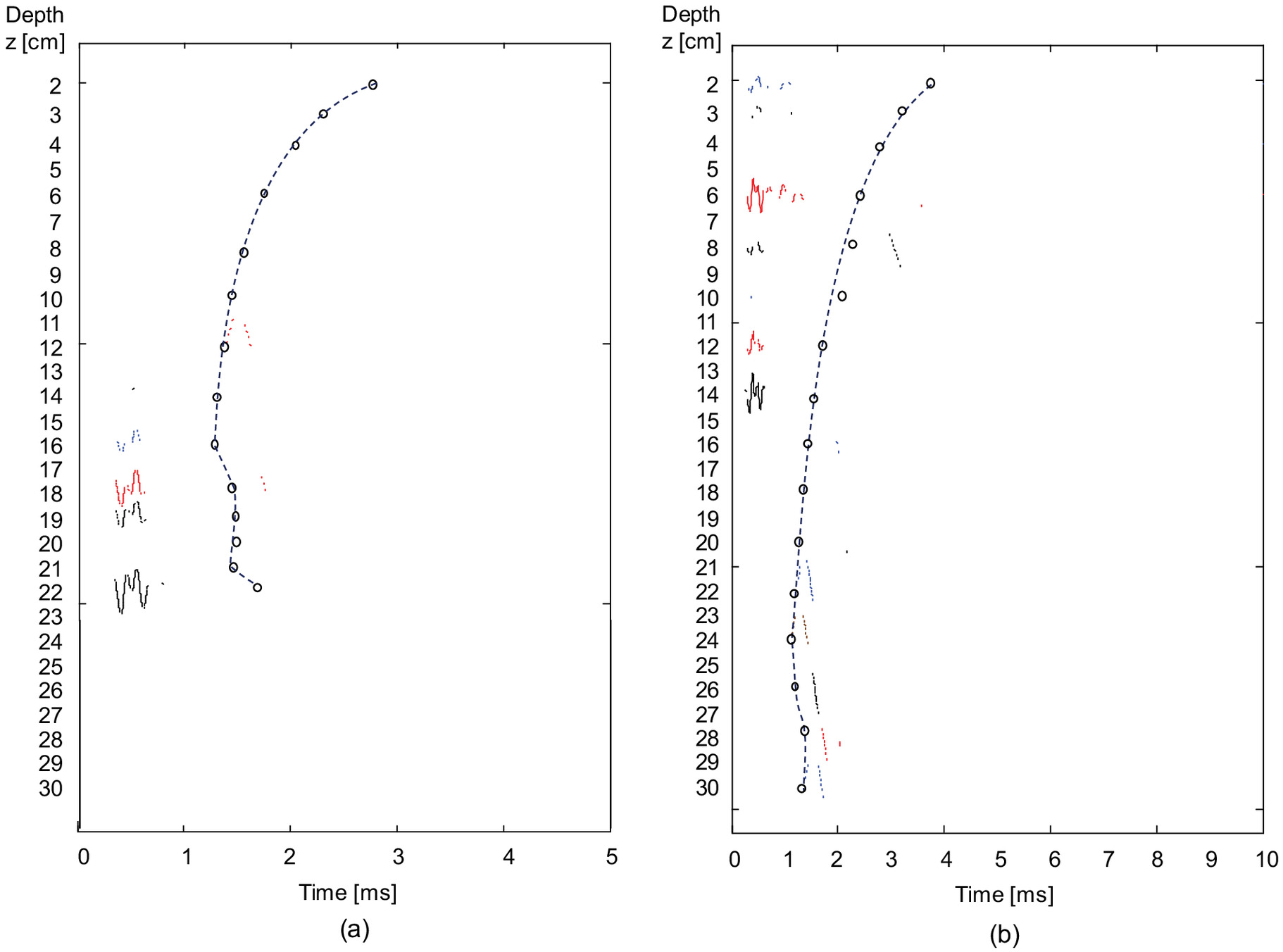
Fig. 6. Shear S-wave signatures versus depth: (a) kaolinite; (b) silt; and (c) fine sand. Note the different time scales for the three sediments.

Fig. 7 shows shear wave signatures with depth gathered at two offshore locations: a silty-sand deposit at South Beach [Fig. 7(a)] and a clayey sediment at the Monument site [Fig. 7(b)]. We used the same testing protocol as in the laboratory: incremental insertion at

2 cm / s

followed by a holding period until measurements exhibited a stable arrival time. Bubbles readily come out upon stirring the sediment bed at the end of the test, and recovered cores show marked layering at the two test locations. Thus, changes in first arrival times with depth reflect changes in the effective stress, layering, and trapped gas.

Fig. 7. Shear wave signature versus depth—field measurements offshore: (a) silty-sand sediment at the South Beach site; and (b) clayey sediment at the Monument site.

Results—Prevalent Trends

The shear wave velocity

V_{s} = L / t_{a}

is the tip-to-tip distance

L

divided by the time to the first arrival

t_{a}

identified for each signal. Fig. 8 summarizes the shear wave velocity versus depth data for shallow sediments measured in the laboratory and in the field as part of this study and includes additional data compiled from the literature. The shear wave velocity increases with depth. Two boundaries separate sandy sediments (higher

V_{s}

values at shallow depths) from clayey sediments (lower

V_{s}

). Data clustering highlights the potential use of

V_{s}

-depth profiles for both stiffness assessments and sediment preclassification.

Fig. 8. Shear wave velocity $V_{S}$ versus depth $z$ . Filled markers indicate data measured in this study (red: kaolinite; green: silica flour; orange: field data at Monument site; yellow: field data at South beach site; blue: fine sand). Other symbols: data gathered from published studies. The blue and red lines are the computed power trend of S-wave velocity as a function of vertical effective stress $σ_{v}^{'}$ and correspond to the two reference silty sediments proposed in Lyu et al. (2021). (Data from Cunny and Fry 1973; Hamilton 1976, 1979; Schultheiss 1981; Lovell and Ogden 1984; Sauter 1987; Gabriels et al. 1987; Muir et al. 1991; Richardson et al. 1991; Stoll 1991; Caiti et al. 1994; Ali and Broadhead 1995; Bibee and Dorman 1995; Liu et al. 1997; Buckingham 2005; Buchanan 2005; Holzer et al. 2005; Klein and Santamarina 2005.)

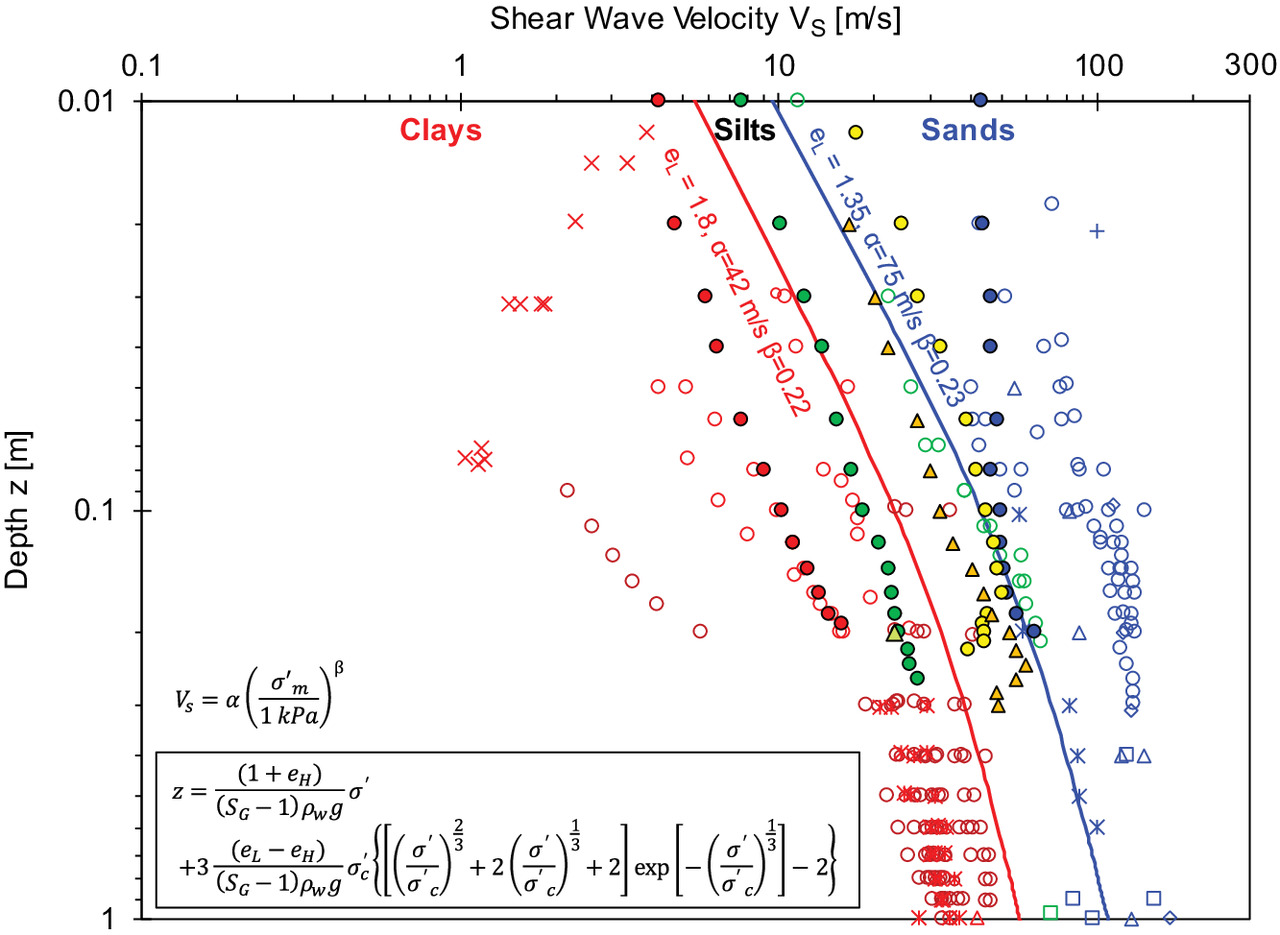
The shear wave velocity in sediments is a power function of the mean effective stress on the polarization plane

σ_{m}^{'}

(Roesler 1979; Knox et al 1982; Yu and Richart 1984; Santamarina and Cascante 1996):

V_{S} = α {(\frac{σ_{m}^{'}}{1 kPa})}^{β}

(7)

where the

α - factor

corresponds to the shear wave velocity at

σ_{m}^{'} = 1 kPa

and the

β - exponent

reflects the sensitivity of the shear wave velocity to changes in effective stress (Cha et al. 2014). Wave measurements during the vertical insertion of the fork probe are based on horizontally-polarized and horizontally-propagating shear waves; therefore, Eq. (7) can be written in terms of the horizontal effective stress

σ_{m}^{'} = σ_{h}^{'}

. The power law relation between

V_{s}

and effective stress

σ^{'}

is confirmed in all cases once the effective stress is computed by integrating density profiles with depth (see the algorithm in Lyu et al. 2021).

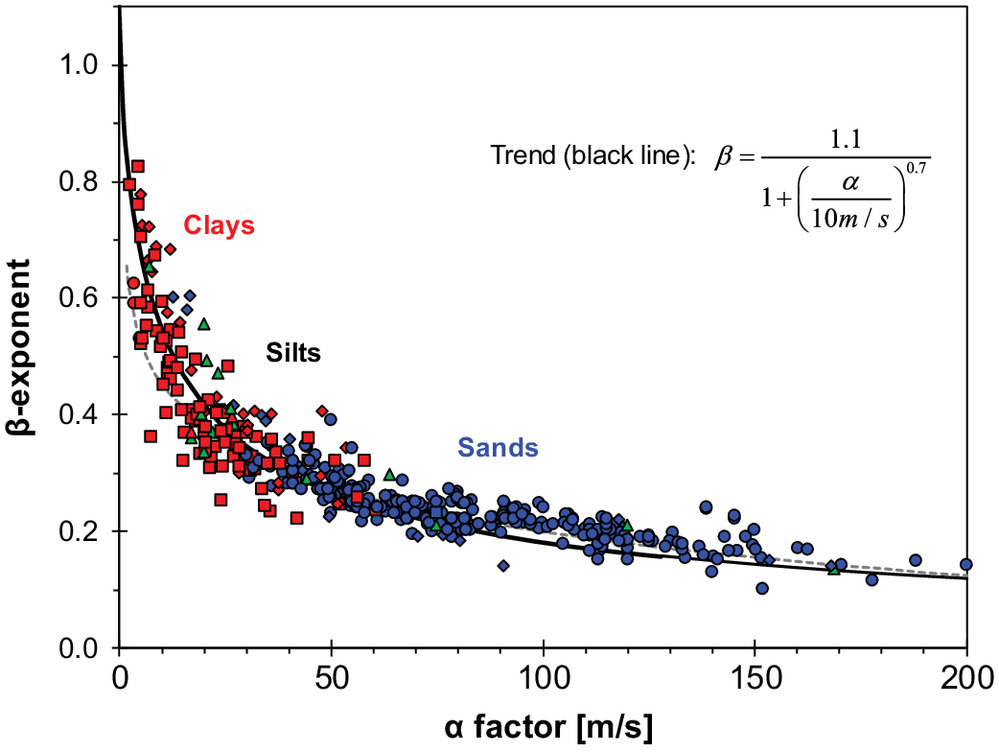
We gathered laboratory and field data and extracted values for the

α

-factor and

β

-exponent [Eq. (7)]. Coarser and denser soils exhibit higher velocity at low stress (

α

-factor) but lower sensitivity to stress changes (

β

-exponent) due to smaller changes in density and coordination number with increasing stress. We confirmed this observation with velocity-stress trends gathered from published studies. Fig. 9 shows the inverse relationship between the

α

-factor and

β

-exponent for different soils including clays, silts, and sands. The newly proposed trend line starts with extremely soft colloidal sediments dominated by electrical interactions (

α = 0

,

β = 1.1

) and ends with cemented rocks where

α = 3,000

-to-

4,000 m / s

and

β < 0.01

[data

n = 479

; root-mean-square error

RMSE = 0.04

- see previous trends in Cha et al. (2014) and Ku et al. (2017)]

β = \frac{1.1}{1 + {(\frac{α}{10 m / s})}^{0.7}}

(8)

Fig. 9. Shear wave velocity as a power function of mean effective stress $V_{s} = α (σ^{'} / kPa)^{β}$ : Relation between the $α$ -factor and the $β$ -exponent for different soil types. Dotted gray line: $α$ - $β$ relationship in Cha et al. (2014). (Data from laboratory and field studies. (Data from Ku 2012; Bate et al. 2013; Cha et al. 2014; Kang et al. 2014; Lee and Santamarina 2005; Ku et al. 2017; Park and Santamarina 2017; Modenesi and Santamarina 2022.)

Effect of Interparticle Electrical Forces

Fluid chemistry-dependent electrical forces govern fabric formation in the water column during the early stages of sedimentation when high specific surface area sediments are involved. Eventually, Terzaghi’s effective stress gains control as the burial depth increases, yet, the fabric retains memory of the formation environment; for example, higher salinity during sediment formation leads to a higher

α

-factor and smaller

β

-exponent [Eq. (7) - Klein and Santamarina 2005; Ku et al. 2011; Kang et al. 2014].

How far does the effect of interparticle electrical forces affect the velocity-stress trends in fine-grained sediments at shallow depth? We replaced the mean effective stress

σ_{m}^{'}

in Eq. (7) for (

σ_{m}^{'} + σ_{A}^{'}

) to include the equivalent effective stress

σ_{A}^{'}

that results from interparticle electrical forces (Sridharan and Rao 1973). Then, we fitted the modified expression to velocity-stress data to infer the

σ_{A}^{'}

value. The effect of electrical forces is indistinguishable in the kaolinites tested in this study (low specific surface area clay,

S_{s} \approx 50 m^{2} / g

). However, we were able to detect it in a very high-plasticity hydrothermal sediment subjected to very low effective stress (liquid limit

L L = 330

, specific surface area

S_{s} = 180 m^{2} / g

); in this case, the computed equivalent effective stress ranged between

σ_{A}^{'} = 1

-and-3.5 kPa (Modenesi and Santamarina 2022). High specific surface sediments form very loose fabrics (Fig. 4) and the effective stress gradient is small; consequently, even a low equivalent effective stress

σ_{A}^{'}

can affect the stiffness of shallow sediments: in the extreme case studied above,

σ_{A}^{'} = 1

-and-3.5 kPa affects the upper 2-to-4 m. The plasticity of most fine-grained sediments is significantly lower and the effect of electrical charges on stiffness will be restricted to the upper few centimeters.

Discussion: Stiffness Profiles and Pressure Diffusion

The sediment self-compaction starts at the sediment-water interface where

σ_{z}^{'} \to 0

and the void ratio

e \to e_{L}

. As depth increases, the effective stress, density, and shear wave velocity increase. Implications on wave propagation, stiffness profiles, and insertion effects are discussed next.

Data Analysis: Ray Bending

The wave velocity increases with depth and is higher in the vertical than the horizontal direction. Then, the wavefront is not spherical in near-surface soils. How does ray bending between the source and the receiver bender elements affect the wave velocities determined using the insertion probe?

Ray-tracing is a two-point boundary value problem; the goal is to identify the ray path that results in the shortest travel time, in agreement with Fermat’s principle. A closed-form solution for the ray path can be obtained using calculus of variation for the following velocity field (Santamarina and Fratta 2005):

•

linearly increasing vertical velocity with depth

V_{v} = a + b \cdot z

•

constant velocity anisotropy

c = V_{v} / V_{h}

where V_h is the horizontal velocity

•

elliptical variation of velocity with ray angle

z^{'} : V (z, z^{'}) = V_{v} (z) \cdot \sqrt{(1 + z^{' 2}) / (c^{2} + z^{' 2})}

where

a

[

m / s

],

b [1 / s]

, and

c [-]

are the model parameters that define the velocity field. Then, the ray depth

z

at position

x

between the source and the receiver is

z = \sqrt{{(\frac{V_{v o}}{b})}^{2} + x [c^{2} (L - x)]} - \frac{a}{b}

(9)

where

V_{v o}

= vertical wave velocity at the depth of the bender elements; and

L

= distance between the source and receiver bender elements. We use Eq. (9) to determine the ray paths at different insertion depths, both in soft clays and stiff sands. We adopt a locally linear velocity profile that is tangent to the true

V_{s} (z)

, and we estimate the velocity anisotropy

c = V_{v} / V_{h}

from the velocity-stress power Eq. (7), in terms of the coefficient of earth pressure at rest

k_{o}

c = \frac{V_{v}}{V_{h}} = \frac{α {[σ_{v} (1 + k_{o})]}^{β}}{α {(2 k_{o} σ_{v})}^{β}} = {(\frac{1 + k_{o}}{2 k_{o}})}^{β}

(10)

The ray paths computed for the probe geometry used in this study show pronounced ray bending at 1 cm depth; however, ray bending decreases rapidly with depth in both soils and is already quite small at 10 cm depth (see Supplemental Materials). The effect of ray bending on the computed wave velocities falls below the uncertainty in first arrival detection within the upper few centimeters: errors in computed velocities are

< 0.4 %

in both sands and clays at 10 cm depth (Note: travel time is the integral of

d ℓ / V_{z, z^{'}}

along the ray path, where

d ℓ

is a differential of the path length).

Small-Strain Stiffness $G_{\max}$ in Depth

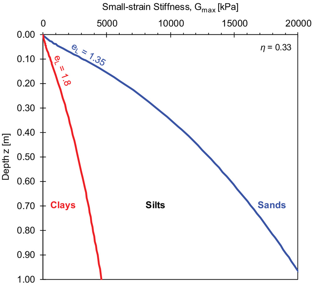
The value of

G_{\max}

depends on fabric-related interparticle coordination and contact stiffness (either flatness due to effective stress, creep and cementation, or electrical interactions such as in clays). We combined the void ratio

e

and shear wave velocity

V_{s}

trends in previous sections to compute the small-strain stiffness

G_{\max} = V_{s}^{2} ρ

profiles with depth. Fig. 10 shows the computed

G_{\max}

boundary profiles that correspond to the shear wave velocity boundaries in Fig. 8, taking into consideration the corresponding density profiles with depth [Eqs. (1) and (3); see model parameters in Fig. 10]. Trends in a linear-linear scale highlight the much faster increase in stiffness with depth for sands as compared to clayey sediments.

Fig. 10. Small-strain stiffness $G_{\max}$ . The blue and red boundaries are computed from the void ratio $e$ and shear wave velocity $V_{s}$ profiles (refer to reference sediments in Lyu et al. 2021). Red line: $e_{L} = 1.8$ , $e_{H} = 0.3$ , $η = 0.33$ , $σ_{c} = 700 kPa$ , $G_{s} = 2.65$ , $α = 42$ , $β = 0.22$ . Blue line: $e_{L} = 1.35$ , $e_{H} = 0.3$ , $η = 0.33$ , $σ_{c} = 1,000 kPa$ , $G_{s} = 2.65$ , $α = 75$ , $β = 0.23$ .

Insertion Effects: Fabric Change and Excess Pore Pressure

The probe tip is designed to displace soil away from the fork tips without affecting the central zone under study, yet, we cannot discard fabric changes [Fig. 5(b)]. Furthermore, velocity transients suggest excess pore pressure generation during probe insertion. We study these two effects next.

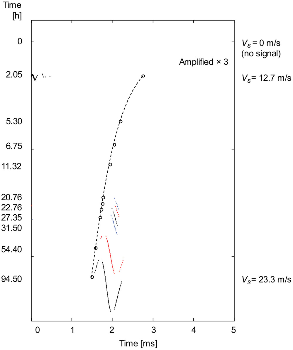
Fabric effects. To investigate fabric effects, we prepared a very dilute silt slurry (silica flour, initial water content

ω > 2,000 %

), deployed the shear wave probe and fixed it 5 cm above the bottom of the large-diameter plexiglass column, and monitored the shear wave signal during self-weight consolidation without displacing the probe. The cascade of shear wave signals in Fig. 11 captures the sediment evolution with elapsed time: the first arrival continuously decreases as effective stress increases during consolidation. At the same sediment depth, the shear wave velocity obtained during probe insertion tests is

V_{s} = 24.0 m / s

, compared to

V_{s} = 23.3 m / s

measured for the undisturbed fabric using the preburied probe. This observation suggests that potential fabric changes caused by probe insertion have minimal effects on the measured

V_{s}

profiles at

z = 20 cm

(at least in silty sediments). In addition, ray bending ahead of the probe may hide any disturbance effects in the upper few centimeters (Supplemental Materials).

Fig. 11. Shear wave signatures: Time evolution during the self-weight consolidation of a silt slurry. The initial water content is $ω > 2,000 %$ . Shear waves measured 5 cm above the bottom ( $z \sim 20 cm$ ). Note: the vertical separation between signals scales with the logarithm of time since sedimentation started.

Excess pore pressure generation. We observed consistent time-dependent changes in travel time after probe insertion (Fig. 12 - Note: the vertical separation between signals scales with the logarithm of time following insertion). In particular, the time to first arrival decreases, and the signal amplitude increases after insertion in clayey and silty sediments, yet opposite transients are observed in sandy sediments (albeit very small). These results suggest that probe insertion causes positive excess pore fluid pressure generation in contractive sediments, and negative excess pressure in dilative soils (note: the generation of excess pore-water pressure was anticipated in both the inner zones of the probe and surrounding areas, then dissipated).

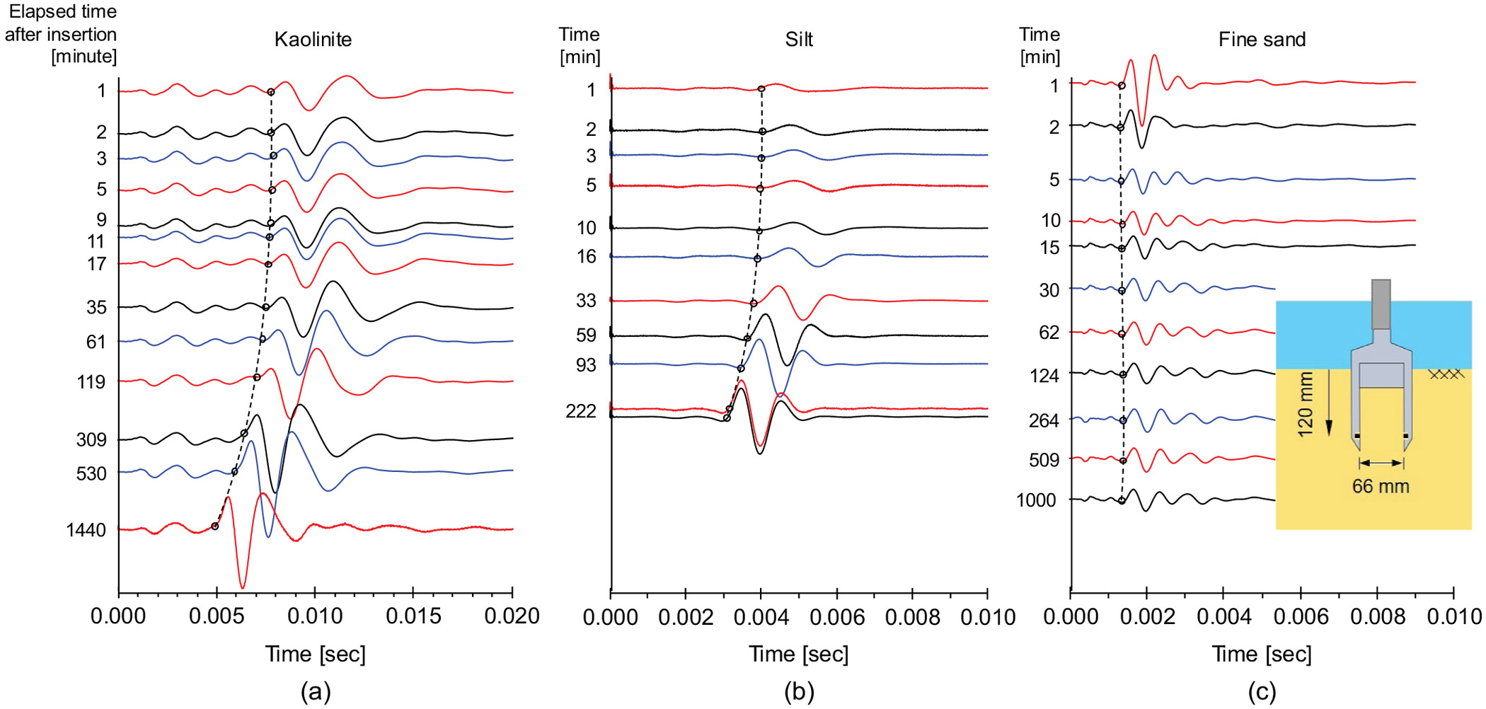
Fig. 12. Pressure diffusion: shear wave signatures versus elapsed time after probe insertion. Data shown for insertion to depth $z = 12 cm$ . (a) Kaolinite; (b) silt; and (c) fine sand. Dashed lines: trends in first arrivals. Note: the vertical separation between signals scales with the logarithm of time since insertion stopped.

Fig. 13(a) presents the evolution of the shear wave velocity

V_{s}

with elapsed time after probe insertion in clay, silt, and sand beds. Salient observations follow:

•

The evolution of the shear wave velocity during pressure diffusion after insertion is both depth- and sediment type-dependent.

•

Velocity changes are quite small in sands (

\sim 7 %

), but they can reach and exceed 100% in shallow clays and silts [Note: Yoon et al. (2008) reported a 7% increase in the shear wave velocity following the probe penetration in soft clay sediments at 30 m depth].

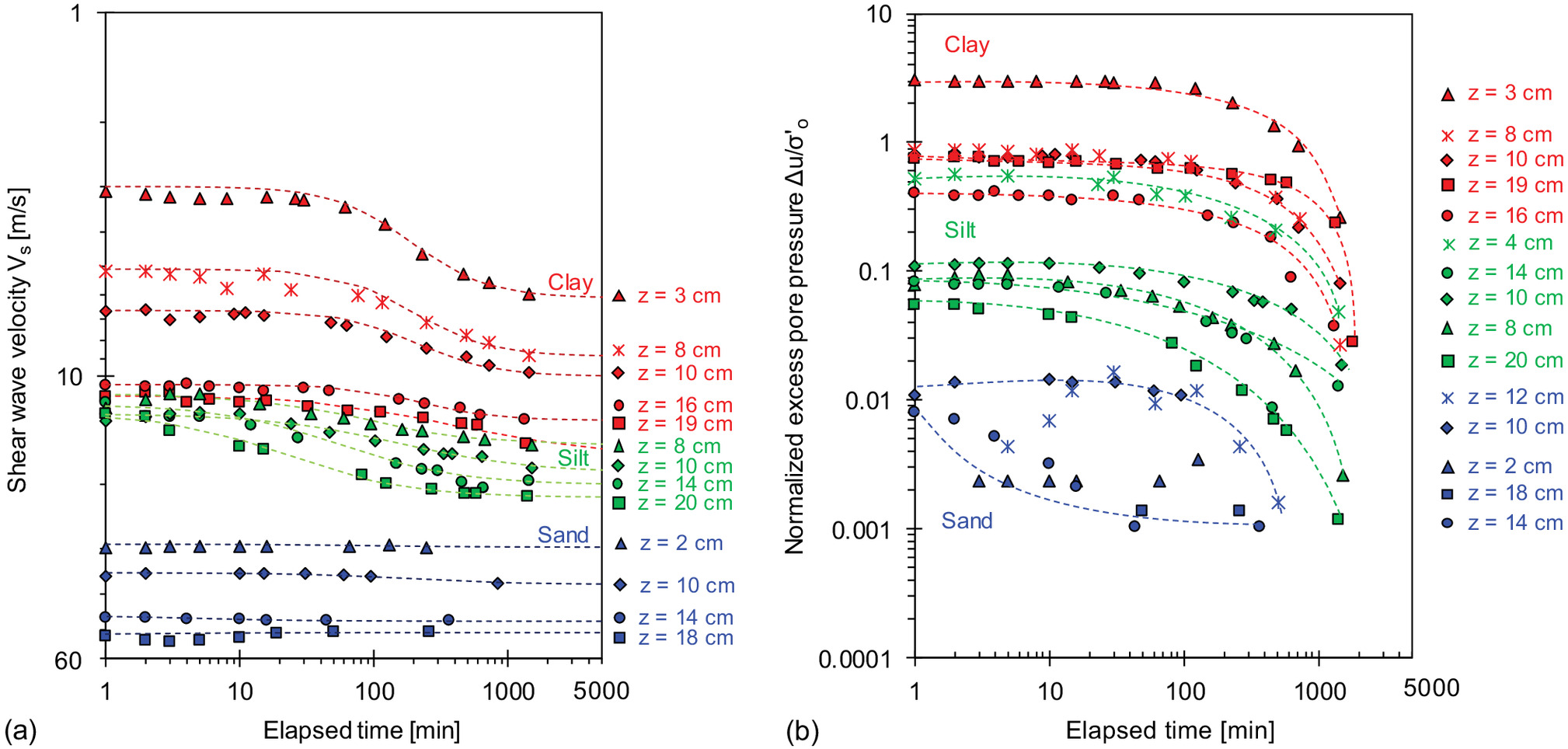
Fig. 13. Pressure diffusion following the probe insertion in clay (red markers), silt (green data points), and sand (blue data points): (a) shear wave velocity $V_{s}$ as a function of time for different insertion depths; and (b) evolution of the excess pore-water pressure $Δ u_{w}$ inferred from shear wave velocity data.

Clearly, the probe insertion causes excess pore fluid pressure

Δ u

and alters the horizontal effective stress

σ_{h}^{'} = σ_{h o}^{'} - Δ u

where

σ_{h o}^{'}

is the initial horizontal effective stress.

Coefficient of consolidation. The sediment-dependent time-varying shear wave velocity trends suggest the possibility of estimating the coefficient of consolidation from these measurements. We followed four steps:

1.

We fitted shear wave velocity versus time data in Fig. 13(a) with a sigmoidal model (logistic function) to reduce the effect of noise on individual measurements (Note:

c^{*}

and

d

are model parameters)

V_{S} (t) = V_{S, t = 0} + \frac{V_{S, t \to \infty} - V_{S, t = 0}}{1 + {(\frac{t}{c^{*}})}^{- \frac{d}{2}}}

(11)

2.

We estimated changes in the effective horizontal stress

{Δ σ^{'}}_{h}

using the power function

{V_{s} = α ({σ^{'}}_{h} / 1 kPa)}^{β}

[Eq. (7).

Clay : α = 33 m / s

and

β = 0.32

.

Silt : α = 58 m / s

and

β = 0.25

. Sand:

α = 110 m / s

and

β = 0.19

].

3.

We assumed

Δ u = - {Δ σ^{'}}_{h}

and determined the evolution of excess pore-water pressure with time. Results in Fig. 13(b) confirm that the time required for excess pore fluid pressure dissipation varies with sediment type (grain size or specific surface area S_s) and can range from a few minutes in clean sands to several hours in clays.

4.

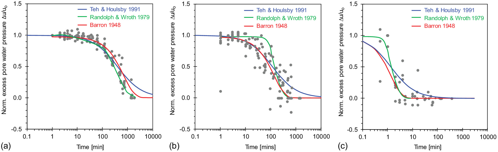
Finally, we used the rate of excess pore fluid pressure dissipation after probe penetration to obtain a first-order estimate of the coefficient of consolidation ch assuming cylindrical drainage along the radial distance r

\frac{\partial u}{\partial t} = c_{h} \frac{\partial^{2} u}{\partial r^{2}} + \frac{c_{h}}{r} \frac{\partial u}{\partial r}

(12)

Solutions for this diffusion equation are summarized in Table 1 and compared in Fig. 14 against data gathered for different sediments; the computed coefficients of consolidation are

c_{h} = 3.5 \times 10^{- 8} m^{2} / s

for clay,

c_{h} = 1 \times 10^{- 7} m^{2} / s

for silt, and

c_{h} = 1 \times 10^{- 5} m^{2} / s

for sand. This analysis makes several simplifying assumptions, including homogeneous excess pore pressure, cylindrical drainage, and uniform shear wave velocity between the source and receiver bender elements. Therefore, the computed coefficients of consolidation are first-order-of-magnitude estimates. Beyond its assumptions, this analysis highlights that data collected during pressure dissipation are valuable for sediment preclassification (see similar efforts for CPT dissipation tests and T-bar analyses—Teh and Houlsby 1991; Burns and Mayne 2002). A detailed evaluation would require more realistic insertion modeling and drainage analysis (e.g., spherical drainage ahead of the tip and preferential drainage above the probe) within a coupled hydromechanical simulator.

Table 1. Diffusion model and solutions

Governing equation	Solution	Method/parameters	References
$\frac{\partial u}{\partial t} = c_{h} \frac{\partial^{2} u}{\partial^{2} r} + \frac{c_{h}}{r} \frac{\partial u}{\partial r}$	$U = u_{o} \frac{n^{2} \ln p - 0.5 (ρ^{2} - 1)}{n^{2} F_{n}} \exp (\frac{- 2 T_{r}}{F_{n}})$	Equal strain consolidation for instantaneous loading	Barron (1948)
	$F_{n} = \frac{n^{2} \ln n}{n^{2} - 1} - \frac{3 n^{2} - 1}{4 n^{2}}$	$u_{o}$ : initial excess water pressure
	$T_{r} = \frac{c_{h} t}{r_{e}^{2}} n = \frac{r_{e}}{r_{w}}$	$c_{h}$ : consolidation coefficient
	$ρ = r / r_{w}$	$r_{e}$ : equivalent radius drainage
	$ρ = r / r_{w}$	$r_{w}$ : radius of drain well
	${\begin{cases} U = \sum B_{n} \exp (- a_{n}^{2} t) C_{o} (λ_{n} r) & r_{o} \leq r \leq r^{} \\ U = 0 & r > r^{} \end{cases}}$	Radial consolidation around a cylindrical cavity/ pore elasticity/ cavity expansion	Randolph and Wroth (1979)
	$B_{n} = \frac{4 c_{u}}{λ_{n}^{2}} \cdot \frac{C_{o} (λ_{n} r_{o}) - C_{o} (λ_{n} R)}{r^{* 2} C_{1}^{2} (λ_{n} r^{*}) - r_{o}^{2} C_{o}^{2} (λ_{n} r_{o})}$	$r_{o}$ : radius of the pile
	$C_{i} (λ_{n} r) = J_{i} (λ r) + μ Y_{i} (λ r)$	$r^{*}$ : radius u is negligibly small
		$S_{u}$ : undrained shear strength
		$C_{o} (λ_{n} r)$ : cylindrical function, where $J_{i}$ and $Y_{i}$ are Bessel functions and $λ r$ is a zero of the Bessel function
	$U = \frac{Δ u}{Δ u_{ref}} \approx \frac{1}{1 + {(T / T_{50})}^{b}}$	Strain path method	Teh and Houlsby (1991)
	$T = c_{h} t / d^{2}$	$c_{h}$ : consolidation coefficient
	$T_{50} = 0.061 I_{r}^{0.5}$	$d$ : diameter of the pile
	$b \approx 0.75$	$S_{u}$ : undrained shear strength
	$I_{r} = G / S_{u}$	$G$ : shear modulus
	$I_{r} = G / S_{u}$	$b$ : exponent

Fig. 14. Normalized excess pore-water pressure versus time after probe insertion and estimated coefficients of consolidation: (a) clay: $c_{h} = 3.5 \times 10^{- 8} m^{2} / s$ ; (b) silt: $c_{h} = 1.0 \times 10^{- 7} m^{2} / s$ ; and (c) sand: $c_{h} = 1.0 \times 10^{- 5} m^{2} / s$ . Gray data points: experimental data. Lines: analytical models in Table 1. (Data from Teh and Houlsby 1991; Randolph and Wroth 1979; Barron 1948.)

Conclusions

This study focused on shallow seafloor sediments at low effective stress using laboratory and field experiments and extensive databases compiled from published studies. It placed emphasis on sediment-dependent self-compaction characteristics starting with the asymptotic void ratio at the interface between the water column and the sediment column, involved the development of an insertion probe for shear wave velocity measurements to assess the evolution of shear stiffness with depth

G_{\max}

, and advanced data analysis protocols to gain valuable sediment characterization information.

•

The asymptotic void ratio e_L is determined by the grain size distribution and the particle shape in coarse-grained soils (sands and silts) and by the mineralogy and pore fluid pH and ionic strength in fine-grained sediments. Overall, the sediment-specific surface area S_s provides a first-order estimate of the asymptotic void ratio e_L, in agreement with simple geometric fabric analyses.

•

The asymptotic void ratio e_L and the sediment compressibility are correlated. Together, they determine the sediment self-compaction, effective stress gradient, and stiffness profile with depth. The asymptotic void ratio e_L obtained from consolidation tests using remolded specimens prepared as soft pastes is smaller than the asymptotic void ratio observed at the seafloor surface. Sedimentation tests with low solid content slurries provide a more realistic estimate of the asymptotic void ratio including the effects of pore fluid chemistry on fabric formation.

•

The shear wave velocity increases with depth and is causally linked to the mean effective stress

{V_{s} = α ({σ^{'}}_{m} / 1 kPa)}^{β}

. The

α

-factor and

β

-exponent depend on the type of interparticle contact (lower

α

and higher

β

in electrical than in Hertzian particle interactions) and the sediment compressibility (more compressible sediments start with a lower

α

but have a higher

β

due to the increase in coordination number with effective stress). The

α

-factor and

β

-exponent are inversely related and vary from

β \to 1.1

and

α \to 0 m / s

for soft colloidal systems, to

β \to 0

and high

α

-factor for cemented soils and rocks (

α \approx 3,000 - to - 4,000 m / s

and

β < 0.01

).

•

The effect of interparticle electrical forces on shear wave velocity profiles is detected in sediments with very high specific surface area and at very low effective stress. The equivalent effective stress due to electrical interactions can reach 1-to-3.5 kPa.

•

Small-strain stiffness

G_{\max} = {V_{s}}^{2} ρ

profiles highlight the rapid increase in stiffness with depth for sands compared to clayey sediments: sands start with a lower asymptotic void ratio at the surface; thus, the accumulation of overburden stress is faster in sands than clays.

•

The ray path between the source and the receiver bends downwards toward the faster velocities. Closed-form solutions for the ray path reveal that ray bending affects the estimated wave velocity in the upper few centimeters only.

•

Probe insertion causes excess pore fluid pressure that alters the effective stress and shear wave velocity. The time required for excess pressure dissipation varies with sediment type, from a few minutes in clean sands to several hours in clays. The rate of V_s changes with time after probe penetration can be used to obtain a first-order estimate of the coefficient of consolidation c_h. Together, shear wave velocity and diffusion time provide valuable information for sediment preclassification and analyses.

Notation

The following symbols are used in this paper:

$a$: parameter in linear velocity fitting ( $m / s$ );
$b$: parameter in linear velocity fitting ( $1 / s$ );
$C_{c}$: coefficient of consolidation;
$C_{u}$: coefficient of uniformity;
$c$: velocity anisotropy;
$c_{h}$: coefficient of consolidation (subscripts: h = radial, v = vertical) ( $m^{2} / s$ );
$c^{*}$: parameter in sigmoidal model;
$d$: parameter sigmoidal model;
$d_{50}$: mean particle size (mm);
$e$: void ratio (subscripts: at 1 kPa, H: at high effective stress, L: at low effective stress);
$e_{\max}$: maximum void ratio;
$G_{\max}$: small-strain shear modulus (Pa);
$G_{s}$: specific gravity;
$k_{o}$: coefficient of earth pressure at rest;
$L$: travel distance (mm);
$L L$: liquid limit (%);
$R$: roundness;
$r$: radius (m);
$S_{s}$: specific surface area ( $m^{2} / g$ );
$t$: time (subscript: o = arrival time) (s);
$u$: pore fluid pressure (subscript: o = hydrostatic) (kPa);
$V_{s}$: shear wave velocity ( $m / s$ );
$w$: water content (%);
$z$: depth (m);
$α - factor$: shear wave velocity at 1 kPa;
$β - exponent$: sensitivity to changes in the effective stress;
$η$: exponent used in consolidation model;
$ρ$: density (subscript: w = water) ( $kg / m^{3}$ );
$σ^{'}$: effective stress (subscripts: c = characteristic, h = horizontal, m = mean, v = vertical) (kPa);
$σ_{A}^{'}$: van der Waals attraction equivalent effective stress (kPa);
$Δ σ^{'}$: change in effective stress (kPa); and
$Δ u$: excess pore fluid pressure (kPa).

Supplemental Materials

File (supplemental_material_jggefk.gteng-10759_ramirez.pdf)

Download
561.88 KB

Data Availability Statement

All data, models, and code generated or used during the study appear in the published article.

Acknowledgments

The closed-form solution for the ray path was originally derived by M. Cesare and J. C. Santamarina. Support for this research was provided by the KAUST Endowment at King Abdullah University of Science and Technology. Gabrielle E. Abelskamp edited the manuscript.

References

Ali, H. B., and M. K. Broadhead. 1995. “Shear wave properties from inversion of Scholte wave data.” In Full field inversion methods in ocean and seismo-acoustics, 371–376. Dordrecht, Netherlands: Springer.

Crossref

Google Scholar

Altuhafi, F. N., M. R. Coop, and V. N. Georgiannou. 2016. “Effect of particle shape on the mechanical behavior of natural sands.” J. Geotech. Geoenviron. Eng. 142 (12): 04016071. https://doi.org/10.1061/(ASCE)GT.1943-5606.0001569.

Google Scholar

Andersen, K. H., H. P. Jostad, and R. Dyvik. 2008. “Penetration resistance of offshore skirted foundations and anchors in dense sand.” J. Geotech. Geoenviron. Eng. 134 (1): 106–116. https://doi.org/10.1061/(ASCE)1090-0241(2008)134:1(106).

Google Scholar

ASTM. 2006. Standard test methods for minimum index density and unit weight of soils and calculation of relative density. ASTM D4254. West Conshohocken, PA: ASTM.

Google Scholar

Barron, R. A. 1948. “Consolidation of fine-grained soils by drain wells by drain wells.” Trans. Am. Soc. Civ. Eng. 113 (1): 718–742. https://doi.org/10.1061/TACEAT.0006098.

Google Scholar

Bate, B., H. Choo, and S. E. Burns. 2013. “Dynamic properties of fine-grained soils engineered with a controlled organic phase.” Soil Dyn. Earthquake Eng. 53 (Oct): 176–186. https://doi.org/10.1016/j.soildyn.2013.07.005.

Google Scholar

Bauer, E. 1996. “Calibration of a comprehensive hypoplastic model for granular materials.” Soils Found. 36 (1): 13–26. https://doi.org/10.3208/sandf.36.13.

Google Scholar

Been, K., and M. G. Jefferies. 1985. “A state parameter for sands.” Géotechnique 35 (2): 99–112. https://doi.org/10.1680/geot.1985.35.2.99.

Google Scholar

Bibee, L. D., and L. M. Dorman. 1995. “Full waveform inversion of seismic interface wave data.” In Full field inversion methods in ocean and seismo-acoustics, 377–382. Dordrecht, Netherlands: Springer.

Crossref

Google Scholar

Buchanan, J. L. 2005. An assessment of the Biot-Stoll model of a poroelastic seabed. Washington, DC: Acoustic Signal Processing Branch.

Google Scholar

Buckingham, M. J. 2005. “Compressional and shear wave properties of marine sediments: Comparisons between theory and data.” J. Acoust. Soc. Am. 117 (1): 137–152. https://doi.org/10.1121/1.1810231.

Google Scholar

Burland, J. B. 1990. “On the compressibility and shear strength of natural clays.” Géotechnique 40 (3): 329–378. https://doi.org/10.1680/geot.1990.40.3.329.

Google Scholar

Burland, J. B., S. Rampello, V. N. Georgiannou, and G. Calabresi. 1996. “A laboratory study of the strength of four stiff clays.” Géotechnique 46 (3): 491–514. https://doi.org/10.1680/geot.1996.46.3.491.

Google Scholar

Burns, S., and P. Mayne. 2002. “Analytical cavity expansion-critical state model for piezocone dissipation in fine-grained soils.” Soils Found. 42 (2): 131–137. https://doi.org/10.3208/sandf.42.2_131.

Google Scholar

Caiti, A., T. Akal, and R. D. Stoll. 1994. “Estimation of shear wave velocity in shallow marine sediments.” IEEE J. Ocean. Eng. 19 (1): 58–72. https://doi.org/10.1109/48.289451.

Google Scholar

Carraro, J. A., M. Prezzi, and R. Salgado. 2009. “Shear strength and stiffness of sands containing plastic or nonplastic fines.” J. Geotech. Geoenviron. Eng. 135 (9): 1167–1178. https://doi.org/10.1061/(ASCE)1090-0241(2009)135:9(1167).

Google Scholar

Cerato, A. B., and A. J. Lutenegger. 2006. “Specimen size and scale effects of direct shear box tests of sands.” Geotech. Test. J. 29 (6): 507–516.

Google Scholar

Cha, M., J. C. Santamarina, H. S. Kim, and G. C. Cho. 2014. “Small-strain stiffness, shear-wave velocity, and soil compressibility.” J. Geotech. Geoenviron. Eng. 140 (10): 06014011. https://doi.org/10.1061/(ASCE)GT.1943-5606.0001157.

Google Scholar

Cha, W. 2021. “Long-term sediment response under repetitive mechanical and environmental loadings.” Ph.D. thesis, Energy Resources and Petroleum Engineering, Physical Science and Engineering Division, KAUST Research Repository.

Google Scholar

Chin, C., J. Chen, I. Hu, D. Yao, and H. Chao. 2006. “Engineering characteristics of Taipei clay.” In Vol. 3 of Proc., 2nd Int. Workshop on Characterisation and Engineering Properties of Natural Soils, 1755–1803. London: Taylor & Francis.

Google Scholar

Cho, G., J. Dodds, and J. C. Santamarina. 2006. “Particle shape effects on packing density, stiffness, and strength: Natural and crushed sands.” J. Geotech. Geoenviron. Eng. 132 (5): 591–602. https://doi.org/10.1061/(ASCE)1090-0241(2006)132:5(591).

Google Scholar

Chong, S., and J. C. Santamarina. 2016. “Soil compressibility models for a wide stress range.” J. Geotech. Geoenviron. Eng. 142 (6): 06016003. https://doi.org/10.1061/(ASCE)GT.1943-5606.0001482.

Google Scholar

Cunny, R. W., and Z. B. Fry. 1973. “Vibratory in situ and laboratory soil moduli compared.” J. Soil Mech. Found. Div. 99 (12): 1055–1076. https://doi.org/10.1061/JSFEAQ.0001969.

Google Scholar

Dai, S., and J. C. Santamarina. 2014. “Sampling disturbance in hydrate-bearing sediment pressure cores: NGHP-01 expedition, Krishna–Godavari Basin example.” Mar. Pet. Geol. 58 (Part A): 178–186. https://doi.org/10.1016/j.marpetgeo.2014.07.013.

Google Scholar

Evans, M. D., and S. Zhou. 1995. “Liquefaction behavior of sand-gravel composites.” J. Geotech. Eng. 121 (3): 287–298. https://doi.org/10.1061/(ASCE)0733-9410(1995)121:3(287).

Google Scholar

Fam, M., and J. C. Santamarina. 1997. “A study of consolidation using mechanical and electromagnetic waves.” Géotechnique 47 (2): 203–219. https://doi.org/10.1680/geot.1997.47.2.203.

Google Scholar

Farrar, D., and J. Coleman. 1967. “The correlation of surface area with other properties of nineteen British clay soils.” J. Soil Sci. 18 (1): 118–124. https://doi.org/10.1111/j.1365-2389.1967.tb01493.x.

Google Scholar

Feng, X., M. F. Randolph, S. Gourvenec, and R. Wallerand. 2014. “Design approach for rectangular mudmats under fully three-dimensional loading.” Géotechnique 64 (1): 51–63. https://doi.org/10.1680/geot.13.P.051.

Google Scholar

Gabriels, P., R. Snieder, and G. Nolet. 1987. “In situ measurements of shear-wave velocity in sediments with higher-mode Rayleigh waves.” Geophys. Prospect. 35 (2): 187–196. https://doi.org/10.1111/j.1365-2478.1987.tb00812.x.

Google Scholar

Gregory, A. S., W. R. Whalley, C. W. Watts, N. R. A. Bird, P. D. Hallett, and A. P. Whitmore. 2006. “Calculation of the compression index and precompression stress from soil compression test data.” Soil Tillage Res. 89 (1): 45–57. https://doi.org/10.1016/j.still.2005.06.012.

Google Scholar

Hamilton, E. L. 1976. “Shear-wave velocity versus depth in marine sediments: A review.” Log Analyst 18 (1): 985–996. https://doi.org/10.1190/1.1440676.

Google Scholar

Hamilton, E. L. 1979. “Vp/Vs and Poisson’s ratios in marine sediments and rocks.” J. Acoust. Soc. Am. 66 (4): 1093–1101. https://doi.org/10.1121/1.383344.

Google Scholar

Hamilton, E. L., H. P. Bucker, D. L. Keir, and J. A. Whitney. 1970. “Velocities of compressional and shear waves in marine sediments determined in situ from a research submersible.” J. Geophys. Res. 75 (20): 4039–4049. https://doi.org/10.1029/JB075i020p04039.

Google Scholar

Hight, D., M. Paul, B. Barras, J. Powell, D. Nash, P. Smith, R. Jardine, and D. Edwards. 2003. “The characterisation of the Bothkennar clay,” In edited by T. S. Tan, K. K. Phoon, D. W. Hight, and S. Lerouiel, 543–597. Lisse, Netherlands: Swets & Zeitlinger.

Google Scholar

Holzer, T. L., M. J. Bennett, T. E. Noce, and J. C. Tinsley III. 2005. “Shear-wave velocity of surficial geologic sediments in northern California: Statistical distributions and depth dependence.” Earthquake Spectra 21 (1): 161–177. https://doi.org/10.1193/1.1852561.

Google Scholar

Hong, Z. S., J. Yin, and Y. J. Cui. 2010. “Compression behavior of reconstituted soils at high initial water contents.” Géotechnique 60 (9): 691–700. https://doi.org/10.1680/geot.09.P.059.

Google Scholar

Hryciw, R. D., J. Zheng, and K. Shetler. 2016. “Particle roundness and sphericity from images of assemblies by chart estimates and computer methods.” J. Geotech. Geoenviron. Eng. 142 (9): 04016038. https://doi.org/10.1061/(ASCE)GT.1943-5606.0001485.

Google Scholar

Ishihara, K. 1993. “Liquefaction and flow failure during earthquakes.” Géotechnique 43 (3): 351–451. https://doi.org/10.1680/geot.1993.43.3.351.

Google Scholar

Jang, J., and J. C. Santamarina. 2016. “Fines classification based on sensitivity to pore-fluid chemistry.” J. Geotech. Geoenviron. Eng. 142 (4): 06015018. https://doi.org/10.1061/(ASCE)GT.1943-5606.0001420.

Google Scholar

Kang, X. 2015. Mechanical characteristics of organically modified fly ash-kaolinite mixtures. Rolla, MO: Missouri Univ. of Science and Technology.

Google Scholar

Kang, X., G. C. Kang, and B. Bate. 2014. “Measurement of stiffness anisotropy in kaolinite using bender element tests in a floating wall consolidometer.” Geotech. Test. J. 37 (5): 869–883. https://doi.org/10.1520/GTJ20120205.

Google Scholar

Klein, K., and J. C. Santamarina. 2005. “Soft sediments: Wave-based characterization.” Int. J. Geomech. 5 (2): 147–157. https://doi.org/10.1061/(ASCE)1532-3641(2005)5:2(147).

Google Scholar

Knox, D. P., K. H. Stokoe, and S. E. Kopperman. 1982. Effect of state of stress on velocity of low-amplitude shear waves propagating along principal stress directions in dry sand. Austin, TX: Civil Engineering Dept., Univ. of Texas at Austin.

Google Scholar

Ku, T. 2012. “Geostatic stress state evaluation by directional shear wave velocities, with application towards geocharacterization at Aiken, SC.” Ph.D. dissertation, School of Civil and Environmental Engineering, Georgia Institute of Technology.

Google Scholar

Ku, T., P. W. Mayne, and B. J. Gutierrez. 2011. “Hierarchy of vs modes and stress-dependency in geomaterials.” In Proc., 5th Int. Symp. on Deformation Characteristics of Geomaterials, 533–540. Amsterdam, Netherlands: IOS Press.

Google Scholar

Ku, T., S. Subramanian, S. W. Moon, and J. Jung. 2017. “Stress dependency of shear-wave velocity measurements in soils.” J. Geotech. Geoenviron. Eng. 143 (2): 04016092. https://doi.org/10.1061/(ASCE)GT.1943-5606.0001592.

Google Scholar

Lee, J. S., and J. C. Santamarina. 2005. “Bender elements: Performance and signal interpretation.” J. Geotech. Geoenviron. Eng. 131 (9): 1063–1070. https://doi.org/10.1061/(ASCE)1090-0241(2005)131:9(1063).

Google Scholar

Lee, J.-S., C. Lee, H.-K. Yoon, and W. Lee. 2009. “Penetration type field velocity probe for soft soils.” J. Geotech. Geoenviron. Eng. 136 (1): 199–206. https://doi.org/10.1061/(ASCE)1090-0241(2010)136:1(199).

Google Scholar

Liu, A. J., and S. R. Nagel. 1998. “Jamming is not just cool any more.” Nature 396 (6706): 21–22. https://doi.org/10.1038/23819.

Google Scholar

Liu, H. P., Y. Hu, J. Dorman, T. S. Chang, and J. M. Chiu. 1997. “Upper Mississippi embayment shallow seismic velocities measured in situ.” Eng. Geol. 46 (3–4): 313–330. https://doi.org/10.1016/S0013-7952(97)00009-4.

Google Scholar

Lovell, M. A., and P. Ogden. 1984. Remote assessment of permeability/thermal diffusivity of consolidated clay sediments. Luxembourg: Directorate-General Science Research and Development.

Google Scholar

Lyu, C., J. Park, and J. C. Santamarina. 2021. “Depth-dependent seabed properties—Geoacoustic assessment.” J. Geotech. Geoenviron. Eng. 147 (1): 04020151. https://doi.org/10.1061/(ASCE)GT.1943-5606.0002426.

Google Scholar

Mayne, P. W., and F. H. Kulhawy. 1982. “Ko-OCR relationships in soil.” J. Geotech. Eng. Div. 108 (6): 851–872. https://doi.org/10.1061/AJGEB6.0001306.

Google Scholar

Mesri, G., and R. E. Olson. 1971. “Consolidation characteristics of montmorillonite.” Géotechnique 21 (4): 341–352. https://doi.org/10.1680/geot.1971.21.4.341.

Google Scholar

Mitchell, J. K., and K. Soga. 2005. Fundamentals of soil behavior. 3rd ed. Hoboken, NJ: Wiley.

Google Scholar

Modenesi, M. C., and J. C. Santamarina. 2022. “Hydrothermal metalliferous sediments in Red Sea deeps: Formation, characterization and properties.” Eng. Geol. 305 (Aug): 106720. https://doi.org/10.1016/j.enggeo.2022.106720.

Google Scholar

Muir, T. G., A. Caiti, J. M. Hovem, T. Akal, M. D. Richardson, and R. D. Stoll. 1991. “Comparison of techniques for shear wave velocity and attenuation measurements.” In Shear waves in marine sediments, 283–294. Dordrecht, Netherlands: Springer.

Crossref

Google Scholar

Murthy, T. G., D. Loukidis, J. Carraro, M. Prezzi, and R. Salgado. 2007. “Undrained monotonic response of clean and silty sands.” Géotechnique 57 (3): 273–288. https://doi.org/10.1680/geot.2007.57.3.273.

Google Scholar

O’Hern, C. S., S. A. Langer, A. J. Liu, and S. R. Nagel. 2001. “Force distributions near jamming and glass transitions.” Phys. Rev. Lett. 86 (1): 111.

Crossref

Google Scholar

Palomino, A. M., and J. C. Santamarina. 2005. “Fabric map for kaolinite: Effects of pH and ionic concentration on behavior.” Clays Clay Miner. 53 (3): 211–223. https://doi.org/10.1346/CCMN.2005.0530302.

Google Scholar

Park, J., and J. C. Santamarina. 2017. “Revised soil classification system for coarse-fine mixtures.” J. Geotech. Geoenviron. Eng. 143 (8): 04017039. https://doi.org/10.1061/(ASCE)GT.1943-5606.0001705.

Google Scholar

Park, J., and J. C. Santamarina. 2020. “The critical role of pore size on depth-dependent microbial cell counts in sediments.” Sci. Rep. 10 (1): 1–7.

Crossref

Google Scholar

Radjai, F., S. Roux, and J. J. Moreau. 1999. “Contact forces in a granular packing.” Chaos 9 (3): 544–550. https://doi.org/10.1063/1.166428.

Google Scholar

Randolph, M. F. 2012. “Offshore design approaches and model tests for sub-failure cyclic loading of foundations.” In Mechanical behaviour of soils under environmentally induced cyclic loads, 441–480. Vienna, Austria: Springer.

Crossref

Google Scholar

Randolph, M. F., and C. Wroth. 1979. “An analytical solution for the consolidation around a driven pile.” Int. J. Numer. Anal. Methods Geomech. 3 (3): 217–229. https://doi.org/10.1002/nag.1610030302.

Google Scholar

Richardson, M. D., E. Muzi, L. Troiano, and B. Miaschi. 1991. “Sediment shear waves: A comparison of in situ and laboratory measurements.” In Microstructure of fine-grained sediments, 403–415. New York: Springer.

Crossref

Google Scholar

Roesler, S. K. 1979. “Anisotropic shear modulus due to stress anisotropy.” J. Geotech. Eng. 105 (7): 871–880.

Crossref

Google Scholar

Russell, E. R., and J. L. Mickle. 1970. “Liquid limit values by soil moisture tension.” J. Soil Mech. Found. Div. 96 (3): 967–989. https://doi.org/10.1061/JSFEAQ.0001428.

Google Scholar

Santamarina, J. C., and G. Cascante. 1996. “Stress anisotropy and wave propagation: A micromechanical view.” Can. Geotech. J. 33 (5): 770–782. https://doi.org/10.1139/t96-102-323.

Google Scholar

Santamarina, J. C., and D. Fratta. 2005. Discrete signals and inverse problems: An introduction for engineers and scientists. Hoboken, NJ: Wiley.

Crossref

Google Scholar

Santamarina, J. C., A. Klein, and M. A. Fam. 2001. Soils and waves: Particulate materials behavior, characterization and process monitoring. New York: Wiley.

Google Scholar

Santamarina, J. C., A. Klein, Y. H. Wang, and E. Prencke. 2002. “Specific surface: Determination and relevance.” Can. Geotech. J. 39 (1): 233–241. https://doi.org/10.1139/t01-077.

Google Scholar

Sauter, A. W. 1987. “Studies of the upper oceanic sea floor using ocean bottom seismometers.” Ph.D. thesis, Scripps Institution of Oceanography, Univ. of California.

Google Scholar

Schultheiss, P. J. 1981. “Simultaneous measurement of P & S wave velocities during conventional laboratory soil testing procedures.” Mar. Georesour. Geotechnol. 4 (4): 343–367.

Crossref

Google Scholar

Simoni, A., and G. T. Houlsby. 2006. “The direct shear strength and dilatancy of sand–gravel mixtures.” Geotech. Geol. Eng. 24 (3): 523–549. https://doi.org/10.1007/s10706-004-5832-6.

Google Scholar

Skempton, A. W. 1970. “First-time slides in over-consolidated clays.” Géotechnique 20 (3): 320–324. https://doi.org/10.1680/geot.1970.20.3.320.

Google Scholar

Sridharan, A., and G. V. Rao. 1973. “Mechanisms controlling volume change of saturated clays and the role of the effective stress concept.” Géotechnique 23 (3): 359–382. https://doi.org/10.1680/geot.1973.23.3.359.

Google Scholar

Stoll, R. D. 1991. “Shear waves in marine sediments—Bridging the gap from theory to field applications.” In Shear waves in marine sediments, 3–12. Dordrecht, Nethelands: Springer.

Crossref

Google Scholar

Studds, P. G., D. I. Stewart, and T. W. Cousens. 1996. The effect of ion valence on the swelling behavior of sodium montmorillonite. Edinburgh, Scotland: Engineering Technics Press.

Google Scholar

Studds, P. G., D. I. Stewart, and T. W. Cousens. 1998. “The effects of salt solutions on the properties of bentonite-sand mixtures.” Clay Miner. 33 (4): 651–660. https://doi.org/10.1180/claymin.1998.033.4.12.

Google Scholar

Sukumaran, B., and A. K. Ashmawy. 2001. “Quantitative characterisation of the geometry of discret particles.” Géotechnique 51 (7): 619–627. https://doi.org/10.1680/geot.2001.51.7.619.

Crossref

Google Scholar

Teh, C. I., and G. T. Houlsby. 1991. “An analytical study of the cone penetration test in clay.” Géotechnique 41 (1): 17–34. https://doi.org/10.1680/geot.1991.41.1.17.

Google Scholar

Terzaghi, K., R. B. Peck, and G. Mesri. 1996. Soil mechanics in engineering practice. New York: Wiley.

Google Scholar

Terzariol, M. 2015. “Laboratory and field characterization of hydrate bearing sediments-implications.” Ph.D. thesis, School of Civil and Environmental Engineering, Georgia Institute of Technology.

Google Scholar

Terzariol, M., J. Park, G. M. Castro, and J. C. Santamarina. 2020. “Methane hydrate-bearing sediments: Pore habit and implications.” Mar. Pet. Geol. 116 (Jun): 104302. https://doi.org/10.1016/j.marpetgeo.2020.104302.

Google Scholar

Thevanayagam, S., T. Shenthan, S. Mohan, and J. Liang. 2002. “Undrained fragility of clean sands, silty sands, and sandy silts.” J. Geotech. Geoenviron. Eng. 128 (10): 849–859. https://doi.org/10.1061/(ASCE)1090-0241(2002)128:10(849).

Google Scholar

Tom, J. G., and D. J. White. 2019. “Drained bearing capacity of shallowly embedded pipelines.” J. Geotech. Geoenviron. Eng. 145 (11): 04019097. https://doi.org/10.1061/(ASCE)GT.1943-5606.0002151.

Google Scholar

Wang, J., G. Li, B. Liu, G. Kan, Z. Sun, X. Meng, and Q. Hua. 2018. “Experimental study of the ballast in situ sediment acoustic measurement system in South China Sea.” Mar. Georesour. Geotechnol. 36 (5): 515–521. https://doi.org/10.1080/1064119X.2017.1348413.

Google Scholar

Yang, S. L., R. Sandven, and L. Grande. 2006. “Instability of sand–silt mixtures.” Soil Dyn. Earthquake Eng. 26 (2–4): 183–190. https://doi.org/10.1016/j.soildyn.2004.11.027.

Google Scholar

Yoon, H.-K., J.-S. Lee, Y.-U. Kim, and S. Yoon. 2008. “Fork blade-type field velocity probe for measuring shear waves.” Mod. Phys. Lett. B 22 (11): 965–969. https://doi.org/10.1142/S0217984908015681.

Google Scholar

Youd, T. L. 1973. “Factors controlling maximum and minimum densities of sands.” In Evaluation of Relative density and its role in geotechnical projects involving cohesionless soils. West Conshohocken, PA: ASTM International.

Crossref

Google Scholar

Yu, P., and F. E. Richart. 1984. “Stress ratio effects on shear modulus of dry sands.” J. Geotech. Eng. 110 (3): 331–345. https://doi.org/10.1061/(ASCE)0733-9410(1984)110:3(331).

Google Scholar

Information & Authors

Information

Published In

Journal of Geotechnical and Geoenvironmental Engineering

Volume 149 • Issue 5 • May 2023

Copyright

This work is made available under the terms of the Creative Commons Attribution 4.0 International license, https://creativecommons.org/licenses/by/4.0/.

History

Received: Jan 29, 2022

Accepted: Oct 25, 2022

Published online: Feb 28, 2023

Published in print: May 1, 2023

Discussion open until: Jul 28, 2023

Authors

Affiliations

Marisol Salva Ramirez https://orcid.org/0000-0002-0169-0918

Postdoctoral Fellow, Earth Science and Engineering, King Abdullah Univ. of Science and Technology (KAUST), Thuwal 23955-6900, Saudi Arabia. ORCID: https://orcid.org/0000-0002-0169-0918

View all articles by this author

Junghee Park https://orcid.org/0000-0001-7033-4653 [email protected]

Assistant Professor, Dept. of Civil and Environmental Engineering, Incheon National Univ., 119 Academy-ro, Yeonsu-gu, Incheon 22012, South Korea (corresponding author). ORCID: https://orcid.org/0000-0001-7033-4653. Email: [email protected]

View all articles by this author

Marco Terzariol https://orcid.org/0000-0001-5362-1968

Research Scientist, Institut français de recherche pour l’exploitation de la mer (IFREMER), Marine Geosciences, Plouzane 29280, France; formerly, King Abdullah Univ. of Science and Technology (KAUST), Thuwal 23955-6900, Saudi Arabia. ORCID: https://orcid.org/0000-0001-5362-1968

View all articles by this author

Jiming Jiang

Research Scientist, CU Beijing Lighting Equipment Co., Ltd., 240 Huixinli Chaoyang District, Beijing 100029, China; formerly, King Abdullah Univ. of Science and Technology (KAUST), Thuwal 23955-6900, Saudi Arabia.

View all articles by this author

J. Carlos Santamarina, A.M.ASCE https://orcid.org/0000-0001-8708-2827

Professor, Earth Science and Engineering, King Abdullah Univ. of Science and Technology (KAUST), Thuwal 23955-6900, Saudi Arabia. ORCID: https://orcid.org/0000-0001-8708-2827

View all articles by this author

Metrics & Citations

Metrics

Citations

Download citation

If you have the appropriate software installed, you can download article citation data to the citation manager of your choice. Simply select your manager software from the list below and click Download.

Cited by

Longde Jin, Andrew Fuggle, Haley Roberts, Christian P. Armstrong, Lina-Maria Pua, Estimating In Situ Shear Wave Velocity Using Machine Learning Techniques, Geo-Congress 2024, 10.1061/9780784485347.044, (436-444), (2024).
Abstract

Abstract

Introduction

In-Situ Density—Asymptotic Void Ratio

Coarse-Grained Sediments—Gravels, Sands, and Silts

Fine-Grained Sediments—Clays

Asymptotic Void Ratio and Compressibility—Caution

Trends as a Function of the Specific Surface Area

Shear Wave Velocity

S-Wave Velocity Probe

Experimental Study: Laboratory and Field

Results—Prevalent Trends

Effect of Interparticle Electrical Forces

Discussion: Stiffness Profiles and Pressure Diffusion

Data Analysis: Ray Bending

Small-Strain Stiffness Gmax in Depth

Insertion Effects: Fabric Change and Excess Pore Pressure

Conclusions

Notation

Supplemental Materials

Data Availability Statement

Acknowledgments

References

Information

Published In

Copyright

History

Authors

Affiliations

Metrics

Citations

Download citation

Cited by

Figures

Other

Share

Copy the content Link

Share with email

Share

Request Username

Create a new account

Change Password

Password Changed Successfully

Verify Phone

Congrats!

Small-Strain Stiffness $G_{\max}$ in Depth