Discrete Structural Systems Modeling: Benchmarking of LS-DEM and LMGC90 with Seismic Experiments
Publication: Journal of Engineering Mechanics
Volume 149, Issue 12
Abstract
Various papers have presented different methods for computations of mechanics and kinematics of discrete structural systems. However, little has been done in comparing and benchmarking the seismic response from two different discrete-system-models with experiments. This paper presents a detailed seismic performance comparison between two models—level set discrete element method (LS-DEM) and Logiciel de Mécanique Gérant le Contact (LMGC90), calibrated with shake table experiments conducted on four concrete-block configurations. Theories of both models are thoroughly explained and compared. The simulation results are benchmarked against experimental data. Finally, the principal results and significance of this benchmarking effort is discussed.
Introduction
The European Organization for Nuclear Research, abbreviated CERN, operates the world’s largest particle physics lab. Their everyday operation, including the use of particle accelerators etc., produces radiation, from which personnel and high-tech equipment need to be shielded. The most usual approach is to use concrete structures of significant mass (Kaplan 1989). CERN uses assemblies of large independent concrete blocks that allow rapid re-configuring for different implementations. However, structures formed from those blocks do not have any joint connecting systems or other protective metal braces between blocks to resist the lateral forces that might be induced in case of earthquakes. Therefore, on top of radiation shielding, CERN needs to guarantee the structural safety of all concrete configurations.
Researches on seismic analysis of rigid bodies without connections date back to decades ago. Monumental articulated ancient Greek and Roman (MAGR) structures consist of members excellently fitting each other without mortar and standing upright only because of gravity and friction. For safety and restoration purposes of those MAGR structures, various researchers have provided valuable insights into the motions of single or multiple rigid bodies under ground excitation and established highly nonlinear governing equation of motions (Sinopoli 1989; Kounadis et al. 2012). However, those equations are not only derived with overly idealized assumptions, but are also limited to specific rigid body configurations and ground excitation patterns. Furthermore, the equation of motion can be made complicated considering energy dissipation happening at the impacting surfaces. Many have shown that the presence of friction may lead to different impact dynamics, as sticking and reverse slipping can happen (Hurmuzlu and Marghitu 1994; Stronge 1991). Therefore, for this study, reliable numerical models with simplified contact mechanics are needed in order to assess the seismic performance of CERN’s many concrete structures.
While an analytical solution is undesirable, and it is impossible to bring every large complicated CERN configuration onto a shake table for seismic analysis, simple concrete configurations can be tested for benchmarking purposes against numerical models. With calibrated numerical models in hand, CERN can confidently simulate current or future concrete-block configurations with various ground excitations and material parameters to probe their seismic performance. With this purpose in mind, in 2019, CERN conducted a test campaign at the Eucentre Foundation, Italy. The dynamic response of four different concrete-block configurations was investigated through seismic tests (Sironi et al. 2023). In this paper, experimental results from the test campaign have been used to calibrate the two discrete-system-model: LS-DEM and LMGC90.
Cundall and Strack (Cundall 1988) introduced the discrete element method (DEM) in 1988, and since then this method has been used extensively for simulations of discrete particles. Traditionally, DEM deals with spherical shaped particles, hence making it inappropriate for applications with nonspherical particles. In 2016, Kawamoto et al. (2016) introduced a variant of DEM, referred to as the level set discrete element method (LS-DEM), and successfully pushed the boundary of the traditional DEM by making LS-DEM suitable for simulations of any arbitrary shaped particles. So far, LS-DEM has been used extensively in simulating the mechanics of granular media (de Macedo et al. 2021; Karapiperis and Andrade 2021; Kawamoto et al. 2018), metamaterials (Wang et al. 2021), and seismic performance analysis (Andrade et al. 2022). In Andrade et al. (2022), LS-DEM was used to assess the seismic stability of multiblock structures and the results were compared to shake table tests. This was the first attempt ever to use LS-DEM for seismic analysis.
Jean-Jacques Moreau introduced the contact dynamics (CD) method in 1984 (Moreau 1994). The method uses a formulation of unilateral contact, shock laws, Coulomb’s friction, inspired by convex analysis. These laws account roughly for the main features of contact and friction, and are relevant in multi-body collections where sophisticated laws cannot be captured exactly. This method was extended to deformable bodies by Jean (1999) and entitled nonsmooth contact dynamics (NSCD). See (Dubois et al. 2018) for more advanced discussions on this method.
In this paper, we present the benchmarking (including calibration) of the preceding state-of-the-art discrete-system-models, LS-DEM and LMGC90, with experiments. The structure of this paper is as follows: First, we will explain and compare the theories of both models. Then the test campaign conducted in Eucentre will be briefly described. Finally, results from the two calibrated models will be presented and compared with experiments, followed by discussions of similarities and differences. We show that the two models after calibration show remarkable resemblance to the experiments, indicating that both models are suitable for future simulations of large complicated concrete structures that cannot be tested on shake tables.
Model Methods and Comparison
LS-DEM
LS-DEM is a variant of the traditional DEM capable of simulating the kinematics and mechanics of a system of particles with arbitrary shapes, made possible by the usage of level set functions as a geometric basis (Kawamoto et al. 2016). For any random-shaped particles, a level set function, , calculates the distance, , between an arbitrary point, , in the space to the nearest surface of the particle [Fig. 1(a)]
(1)
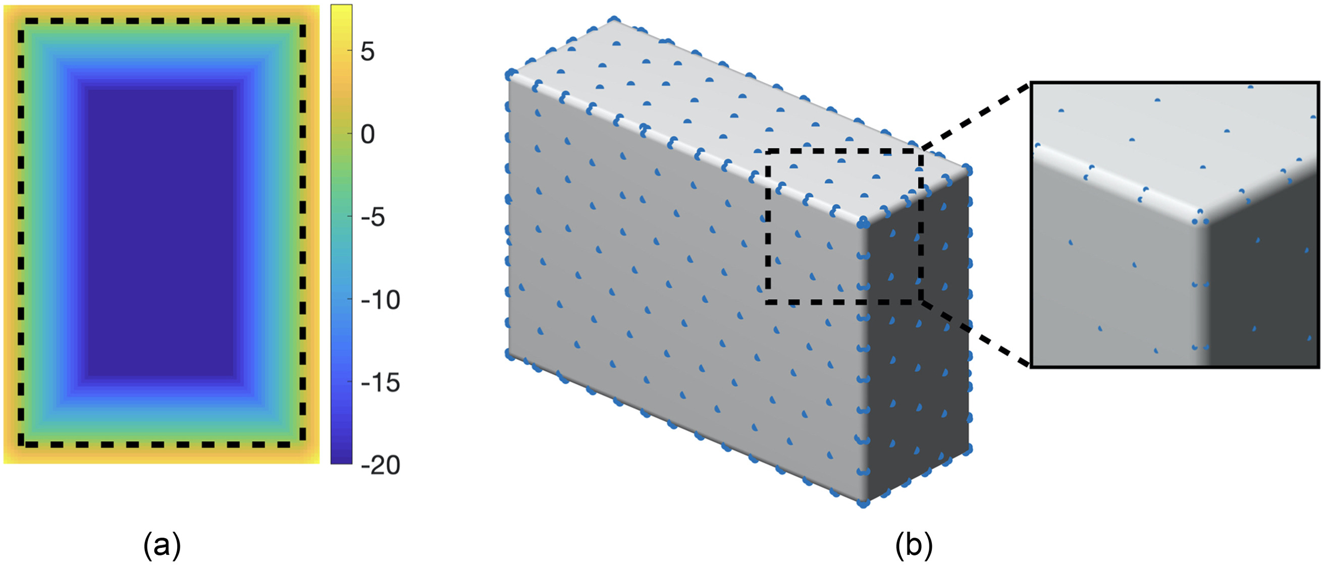
If this point is taken inside the particle, the level set value would be negative. Vice versa, the value would be positive. The surface of the particle can simply be reconstructed using . In this paper, all particles are blocks of same size with a chamfer of 2 cm along the edges.
Together with the level set values, a set of surface point discretization is made to detect particle-to-particle contact [Fig. 1(b)]. In this study, the level set grid had an equal spacing of 0.02m. The surface node had a spacing of roughly 0.2 m.
All surface points of a particle is checked against the level set values of the other particle. If a point has contact, force in normal direction is subsequently calculated usingwhere = normal stiffness of the block, = surface normal calculated at , = critical normal damping coefficient calculated from the coefficient of restitution at the contacting surface point (Harmon et al. 2022, 2021), and = relative velocity of this particle with respect to the other particle.
(2)
Many researchers have proposed different formulas in applying damping to contacting points. For example, Chatzis and Smyth adopted a method in relating damping coefficient to the modulus and density of the contacting medium (Chatzis and Smyth 2012). LS-DEM uses a formula initially proposed by Tsuji el al., incorporating coefficient of restitution directly into a critically damped mass-spring system (Tsuji et al. 1993) bywhere = mass of the colliding object.
(3)
Due to history dependence, shear force is calculated incrementally usingwhere = shear stiffness of the block, and = integrating time step. The ultimate shear force is updated by the smaller value between the build up of incremental shearing force and the critical limit for sliding as proposed by the selection of friction law. In this version of LS-DEM, Coulomb friction law is implemented. Hence, the critical limit for sliding to happen is a fraction of the normal force. The calculation of the updated shearing force at each time step can be represented using the following equation:
(4)
(5)
Both the shear force and the normal force contribute to the moment of the block by crossing with the relative distance with respect to the center of mass of the block, ,
(6)
With all forces and moments calculated, particles are then updated using Newton-Euler equations in explicit scheme with a constant time step that guarantees stability (Tu and Andrade 2008). In this study, the time step of LS-DEM was 0.00001s.
LMGC90
In nonsmooth contact dynamics (NSCD), the contact laws are managed as nondifferentiable steep laws using a nonsmooth dynamics formalism. They are integrated with an implicit scheme, leading to a nonlinear system which is solved using a nonlinear Gauss–Seidel algorithm (NLGS) at each time step. The method uses large time steps (larger than smooth DEM), but each time step is computationally involved due to integration scheme. So in contrast to the previous smooth and explicit DEM, the CD method is a nonsmooth and implicit method. Since rigid contacts are used, no damping has to be introduced. Note that implicit methods enable the correct computation of equilibrium states, which is not always the case with explicit methods. NSCD can also conserve, with a suitable choice of parameters, the total energy of the system in discrete time.
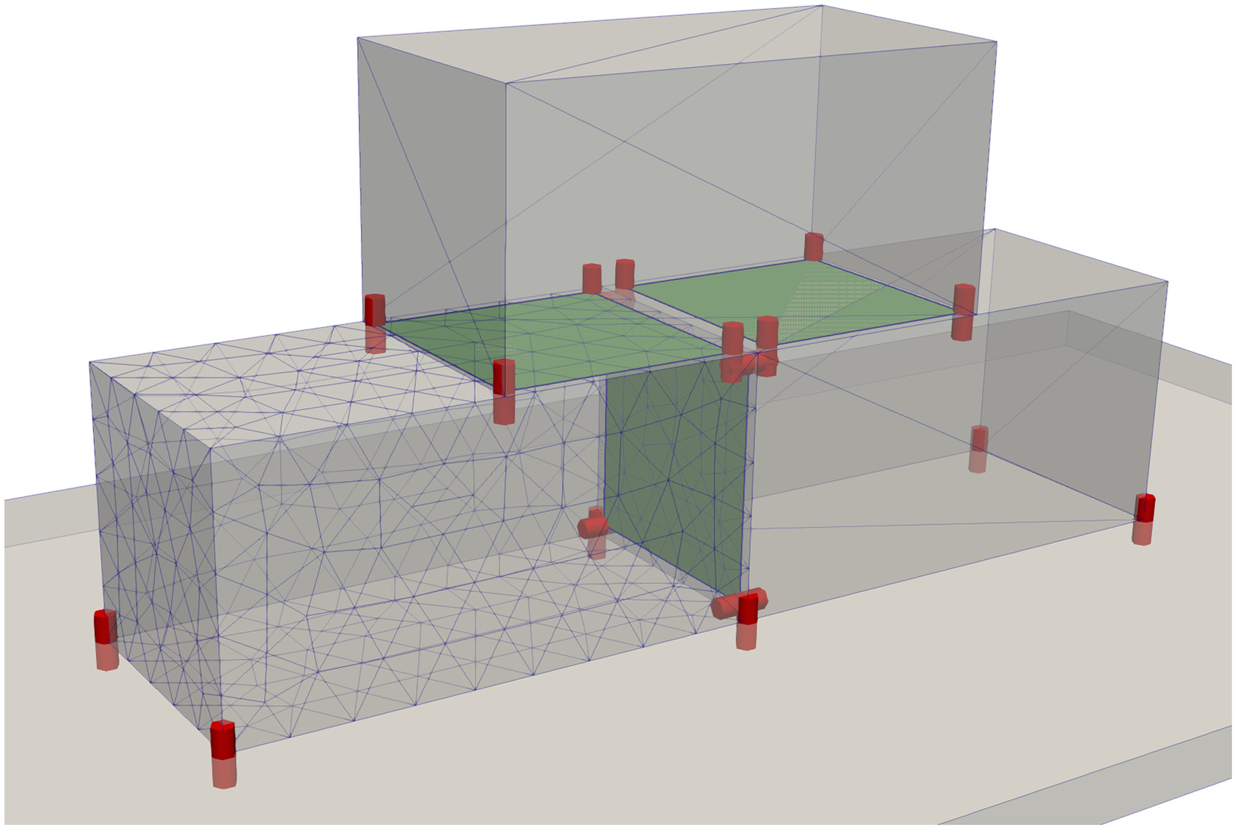
Concerning the modeling of structures made of regular blocks, several approaches are possible. One can consider rigid blocks with frictional contact (Chetouane et al. 2005), or deformable blocks with cohesive frictional contact (Venzal et al. 2020), or any mix of bulk and contacting models. From a technical point of view, depending on the bulk model, the contact conditions are not treated in the same way. For rigid blocks, a common plane approach is used (Cundall 1988), leading to a maximum of 4 contact points (marked by red in Fig. 2). Contact surfaces between blocks (marked by green in Fig. 2), delimited by the four contact points, are shrunk to introduce a kind of safety coefficient. Rigid convex objects are described by a surface mesh. The contact detection algorithm is independent of the mesh as the algorithm looks for overlapping parts of surfaces. For deformable or rigid non convex objects, additional surface nodes are added to the skin mesh to detect contact with other objects in a way similar to LS-DEM. Contact conditions are verified at those surface nodes.
In this paper, simulations were done both with rigid and deformable (elastic and viscoelastic) blocks with frictional contact and no restitution. The mesh size was 0.2m. The time step chosen was 0.001s.
Comparison
Both aforementioned models solve Newton-Euler equations. LS-DEM uses a smooth explicit time integration scheme with a fixed time step. Due to the presence of interpenetration in cases of collision, penalty terms like normal stiffness and shear stiffness are required. The normal force is a function of the interpenetration distance . When the distance is positive, normal force is zero; when the distance is negative, indicating there is a contact, is a linear function of the normal stiffness with respect to . The Coulomb’s friction law adopted in LS-DEM has finite steepness. In case of static friction, i.e., , is a linear function of and . Fig. 3(a) shows a graphical representation of the calculation of and .
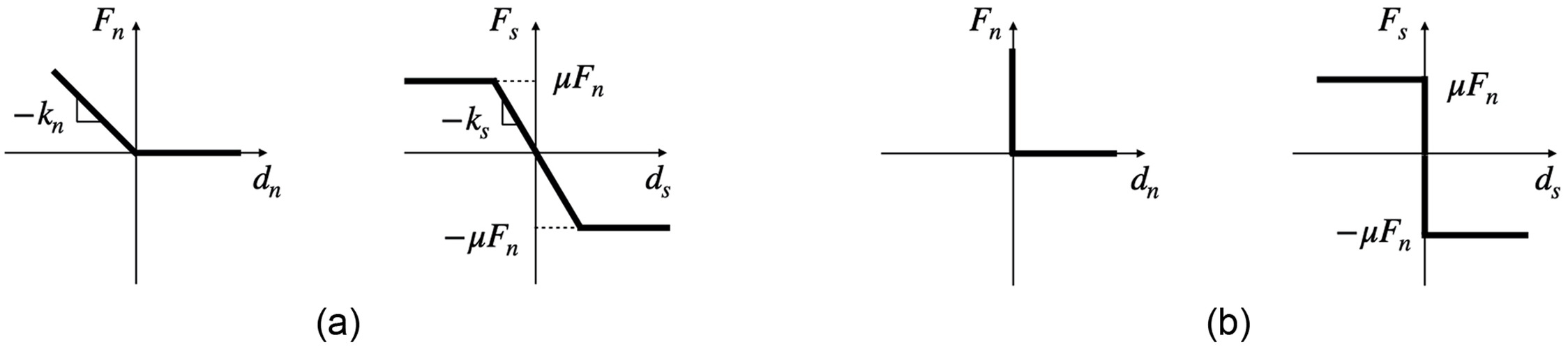
Since the current version of LS-DEM models rigid-body motions, for a fair comparison, only the dynamics of rigid bodies of LMGC90 will be discussed. LMGC90 uses nonsmooth implicit scheme with the equations of motions expressed in differential inclusions (Donze et al. 2009). Unlike LS-DEM, no elastic modulus is required. The term nonsmoothness is an accurate representation of the infinite steepness presented by the inelastic shock law and Coulomb’s law, as in Fig. 3(b). When is positive, the normal force is zero. What’s different from LS-DEM is that when , the Signorini condition ensures that is positive or null. Similarly, the graph of Coulomb friction law exhibits an infinite steep around . Because LMGC90 uses implicit scheme, the choice of time step can be large. At each time step, NLGS is run until convergence, hence each time step can be very time consuming. As a benefit of the implicit scheme, oftentimes energy conservation and numeric stability can be achieved without the use of damping.
Case Study: Rocking Tests
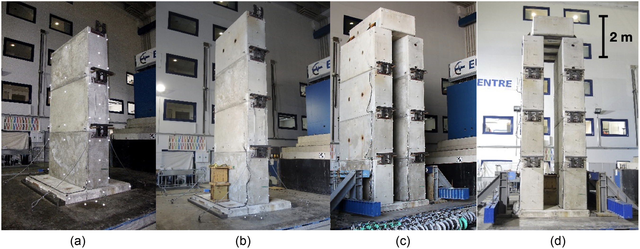
The dynamic response and the stability of four different configurations of stacked concrete blocks were investigated within an experimental campaign consisting of seismic tests. Four different specimens, whose height varied from 4.8 m to about 7.6 m, consisted of a maximum of 9 blocks were constructed (Fig. 4). A wall of three and four stacked blocks, respectively, characterized the first and the second configuration. The third and the fourth one is consisted of two walls of four stacked blocks, with a block at the top; in the fourth specimen, a extra system of steel beams supported the top block.
The specimens were assembled on the steel platform of an unidirectional shake table at the Eucentre Foundation (Pavia, Italy). A base concrete slab, whose translation was restrained by two steel profiles fixed to the platform of the shaking table, simply supported the specimens. Steel stoppers at the base and retaining steel systems provided along the height of the specimens were used to prevent unsafe effects due to unexpected large displacements or rotations. Both the stoppers and the retaining systems were designed not to interfere with the test results.
Accelerations were applied at the base of the specimens. Two different acceleration time-histories, each called Alkion and Basso Tirreno (Ambraseys et al. 2002), were used. They were chosen because they represent an upper bound for a standard acceleration time-history representing the Geneva area, according to the SIA norms (Swiss Society of Engineers and Architects 2020). The acceleration time-histories and their characteristics can be found in Fig. 5 and Table 1.
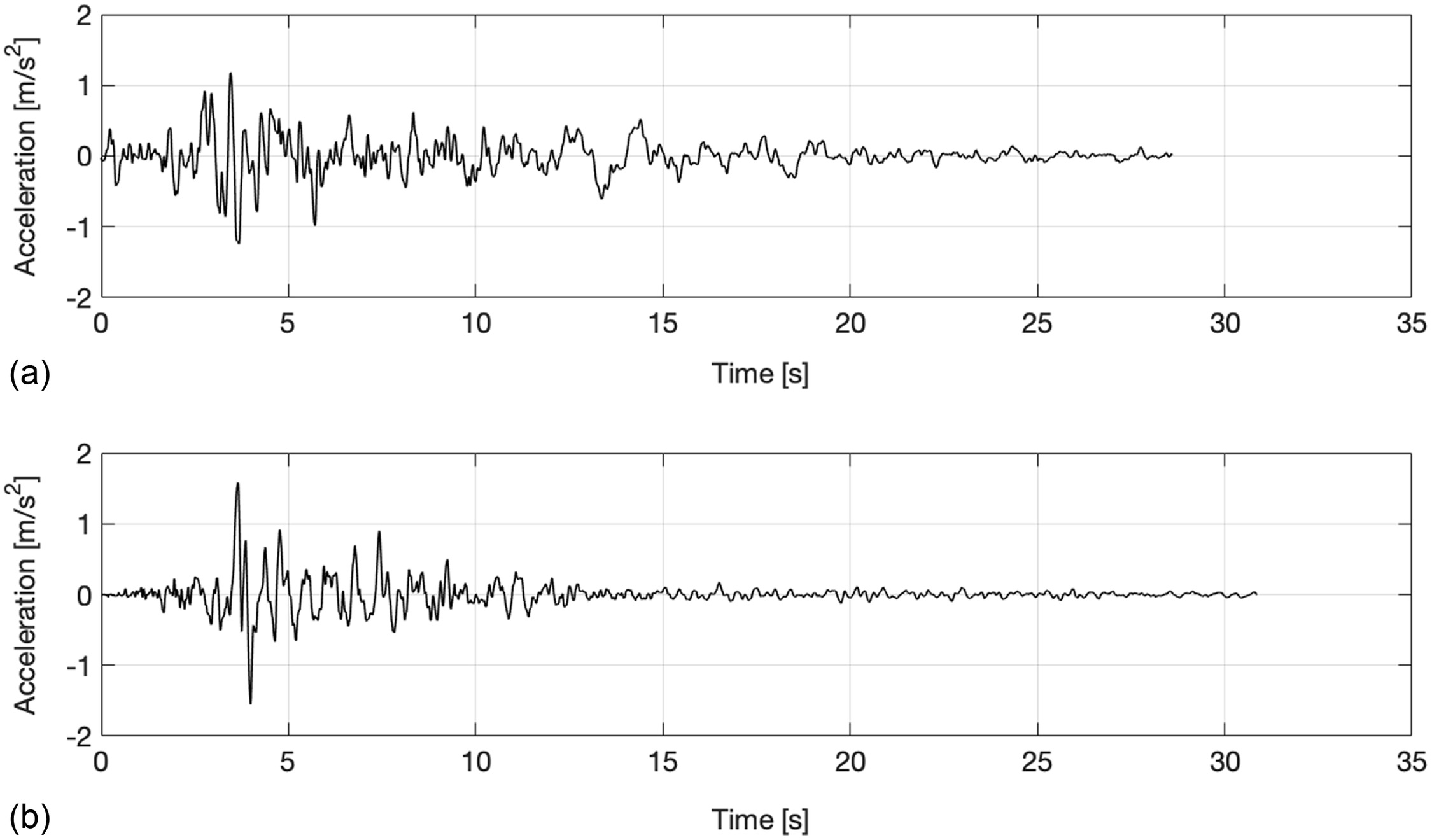
| Earthquake | Date | Magnitude (Mw) | Distance (km) | PGA () |
|---|---|---|---|---|
| Alkion | February 25, 1981 | 6.3 | 25 | 1.176 |
| Basso Tirreno | April 15, 1978 | 6 | 18 | 1.585 |
For each specimen, the first test was performed at a scaled acceleration intensity of 50%. Then a series of successive tests with acceleration amplitude increment of about 25% were performed, until a potential occurrence of structural collapse. At each intensity level, the relative position of each block was checked and, in case of large misalignment, the specimen was restored to its initial configuration. Additional low-intensity constant-amplitude tests with sinusoidal waves were performed at the beginning of the campaign or between two tests with the aim of assessing the dynamic properties and the state of damage of the specimens.
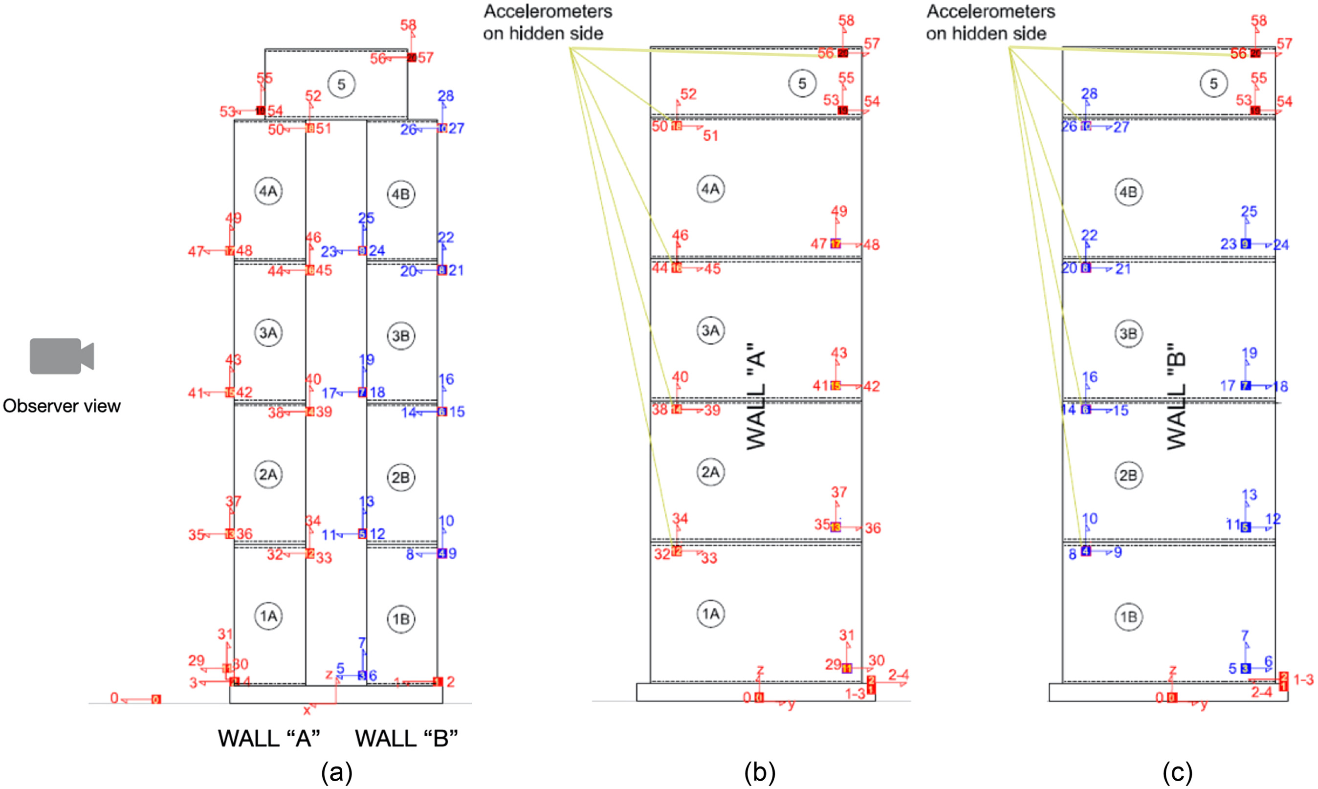
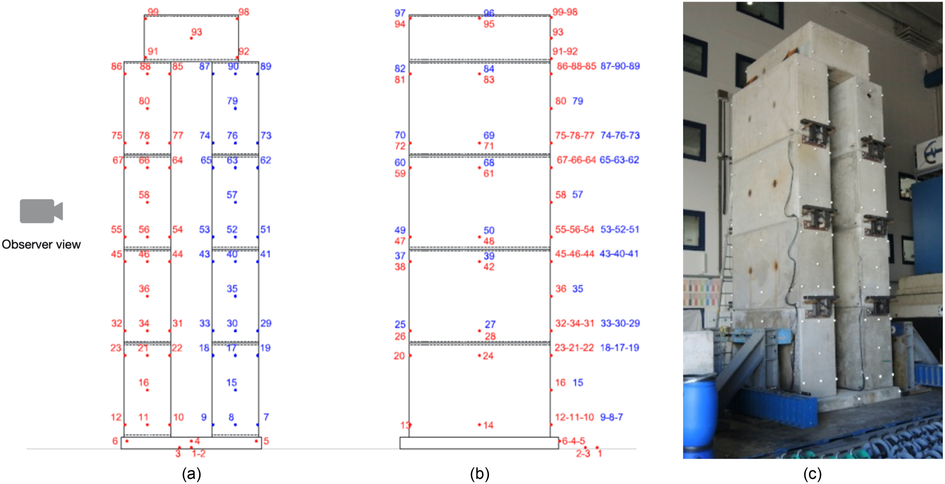
The assessment of the dynamic properties and of the seismic response of the specimens were based on the spatial components of accelerations and displacements measured at different levels along the height of the specimens. The specimens were equipped with up to 21 acceleration transducers, 4 displacement transducers and 101 retro-reflective optical markers, belonging to two different acquisition systems. Further data regarding force, accelerations, velocities and displacements of the shaking table was obtainable from the control system. The measurement frequencies were 512 Hz and 200 Hz for accelerations and displacements, respectively. The acceleration signals were later filtered with a 50Hz-low-pass filter. An example of the layout of the instrumentation is depicted in Figs. 6 and 7 for configuration 3. For more details of the experiments, please refer to Sironi et al. (2023).
Results and Discussion
Model Calibration
To calibrate both models with respect to experiment results of Eucentre’s test campaign, mechanical properties of concrete and steel are required. While most of the distribution parameters of these properties (e.g. mean, standard deviation, or coefficient of variation) can be found in literature, concrete-to-concrete friction coefficient could not be determined due to its large variation present in literature. Therefore, a semiprobabilistic approach using Monte Carlo sampling was adopted.
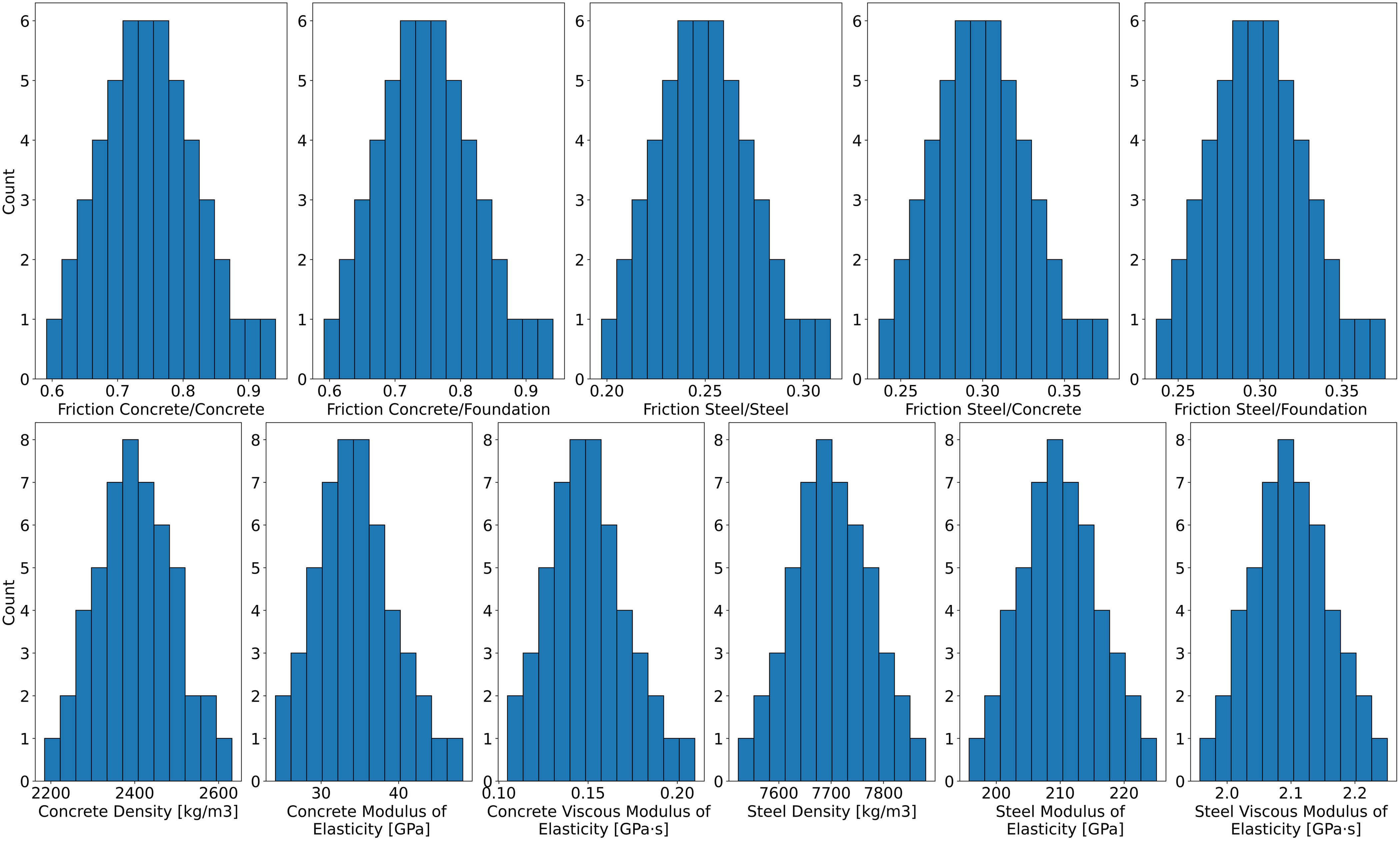
With most of the distribution parameters of concrete and steel properties taken from literature (JCSS 2000, 2001), the mean of concrete-to-concrete friction coefficient was randomly sampled from 0.3 to 0.8. Log-normal distributions were then created for each of the material properties and were later inputted into a procedure based on correlation controlled Latin hypercube sampling (LHS) technique, developed by Vořechovský and Novák (2009), to sample from multivariate distributions. This method is efficient for small sample sizes and can lead to accurate estimates of real behaviors with low variability. In total of 50 sample vectors were produced from this procedure, with each of the sample vectors assembled by sampled properties of concrete and steel (e.g., friction coefficients, density, and modulus of elasticity). Then, 50 sets of simulations (one for each sample vector) were performed in both LS-DEM and LMGC90 in order to determine whether the displacement envelope created by all samples contain the actual experiment data. This process was repeated multiple times to obtain the most optimal value of the mean of concrete-to-concrete friction coefficient. Eventually, a final set of distribution parameters was chosen to be used for future simulations for seismic risk assessment of concrete configurations at CERN.
The optimal values for the distribution parameters of concrete and steel properties are reported in Table 2. For each variable, the histogram of the samples obtained by the LHS technique is presented in Fig. 8.
| Variable | Distribution model | Mean | SD | COV |
|---|---|---|---|---|
| Friction concrete/concrete | Log-normal | 0.75 | 0.075 | 0.1 |
| Friction concrete/foundation | Log-normal | 0.75 | 0.075 | 0.1 |
| Friction steel/concrete | Log-normal | 0.3 | 0.03 | 0.1 |
| Concrete density () | Log-normal | 2,400 | 96 | 0.04 |
| Concrete Young’s modulus (Pa) | Log-normal | 0.15 | ||
| Concrete viscous modulus (Pa) | Log-normal | 0.15 | ||
| Steel density () | Log-normal | 7,700 | 77 | 0.01 |
| Steel Young’s modulus (Pa) | Log-normal | 0.03 | ||
| Steel viscous modulus (Pa) | Log-normal | 0.03 |
While variables like friction coefficient and density are straight forward and universal, there are a couple of parameters that need to be translated or calibrated uniquely in LS-DEM. Normal stiffness and shear stiffness are penalty parameters unique to the DEM. Methods like the Hertzian contact theory directly correlates the elastic modulus of a material to the stiffnesses required in the DEM. However, the Hertzian contact model does not apply for contacts between blocks. Therefore, a different method has to be developed in order to approximate stiffness from real material properties like modulus of elasticity.
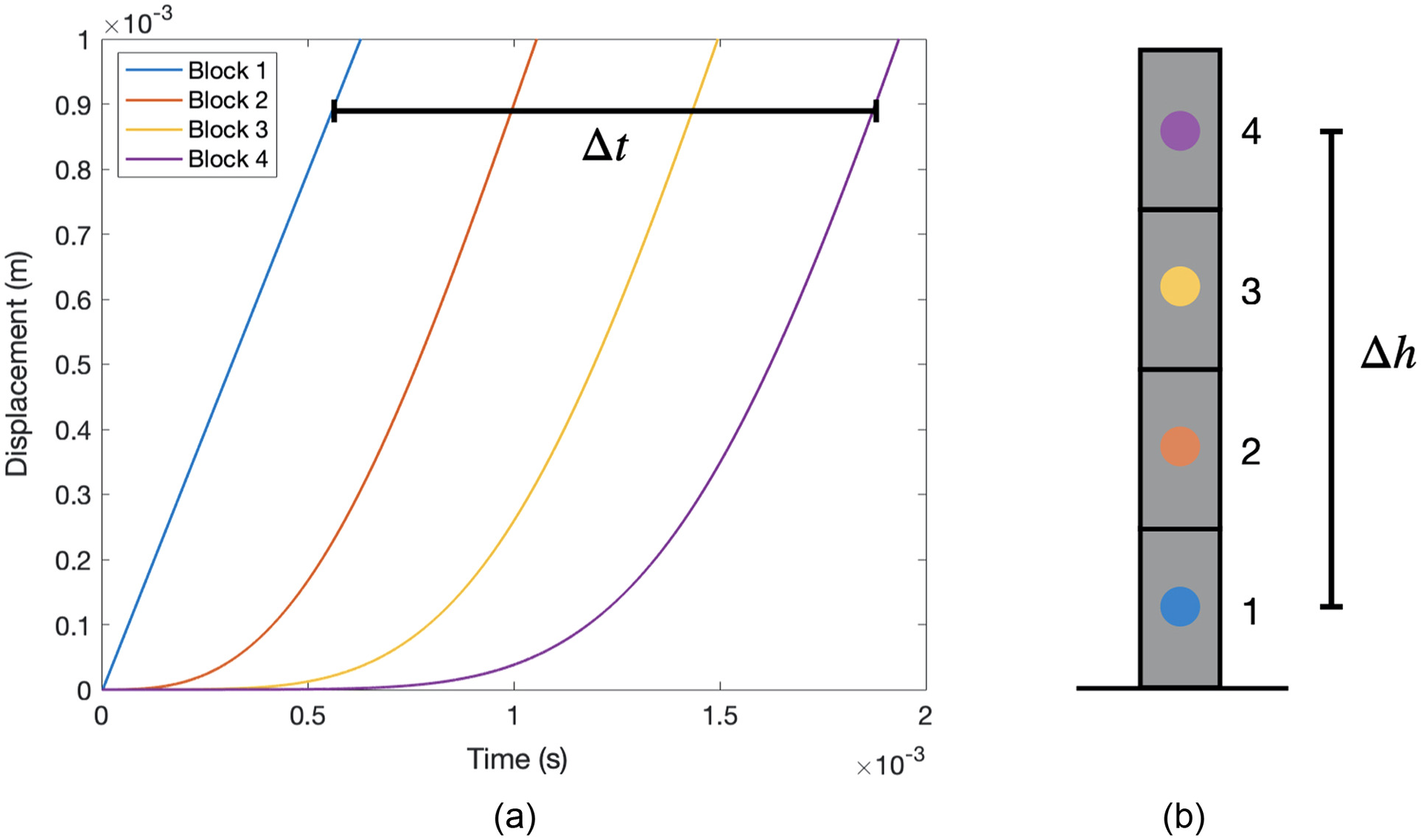
Harmon et al. (2022) presented a novel way of determining and . In reality, when a stack of concrete block assembly is excited by ground acceleration, the motion of blocks is set off via the propagation of stress waves. There is no way to model stress waves in LS-DEM, yet delayed responses of higher blocks are observed due to the presence of contact elasticity. As a result, normal stiffness and shear stiffness can be tuned such that the speed of propagation of motion, referred to as the effective wave speed, in the simulation is the same as the speed of stress wave propagation in reality.
The speed of stress waves can be calculated asfor pressure waves andfor shear waves, where is the Young’s modulus of the material, is the shear modulus and is the density. To match with the preceding speeds, a tower of stacked concrete blocks is set up in the simulation. A unit step of velocity is then given to the ground in LS-DEM in both horizontal and vertical direction respectively. The resulted displacement of the blocks is plotted against time, as shown in Fig. 9. The effective wave speed is calculated after all the blocks have reached a similar velocity, which is indicated by a near-identical slope in Fig. 9. The effective wave speed can then be obtained by .
(7)
(8)
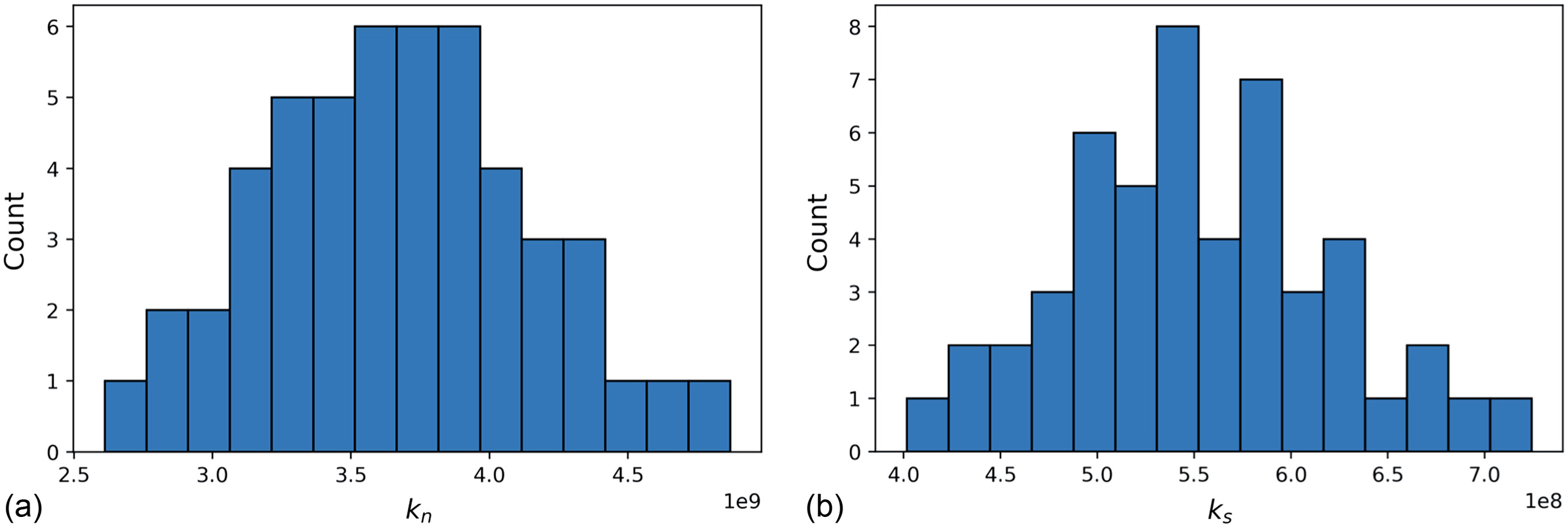
By calculating the effective wave speed and matching it to the actual stress wave propagation speed in Eqs. (7) and (8), one can approximate and . The resulting histograms of such parameters are shown in Fig. 10. We see that the distributions of and do not necessarily follow those of and because the effective wave speed is also affected by block mass. With heavier blocks, larger stiffness is required for the contact to overcome the inertial force and respond to the ground excitation.
Other than the variables listed in Table 2, LS-DEM is taking the coefficient of restitution into the calculation of normal forces [Eq. (2)]. After tuning the model, it is found that a moderate amount of normal damping with is needed in order to compensate for the large obtained due to the significant mass of the blocks. The coefficient of restitution adopted in this paper is within the range reported from Harmon et al. (2022).
In order to examine both methods’ abilities to capture the seismic performance of the concrete structures, tests with the largest ground accelerations were chosen among all the experiments. Displacement readings were taken from the optical marker located at the face center of the side of the base concrete slab. Velocities were then calculated from the displacements and fed into the program as ground input.
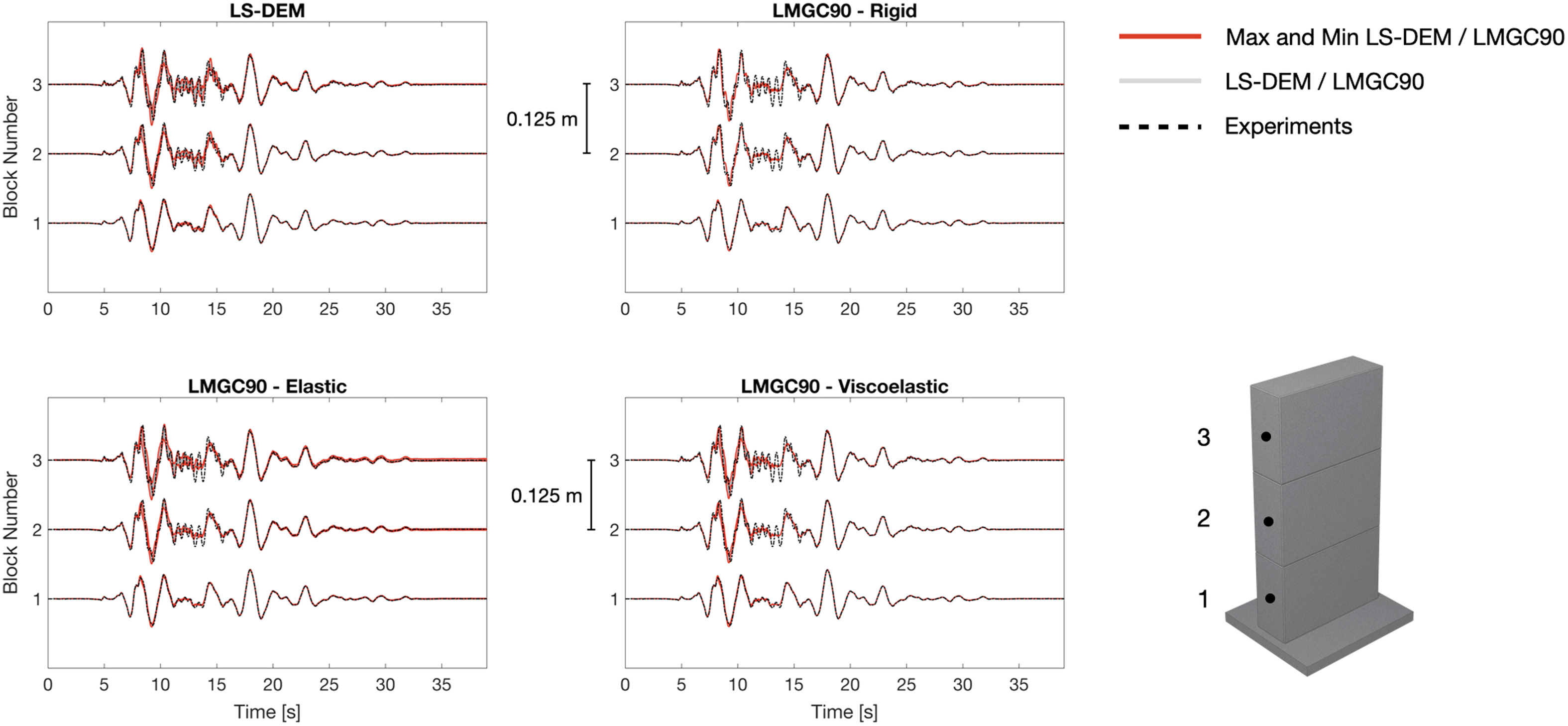
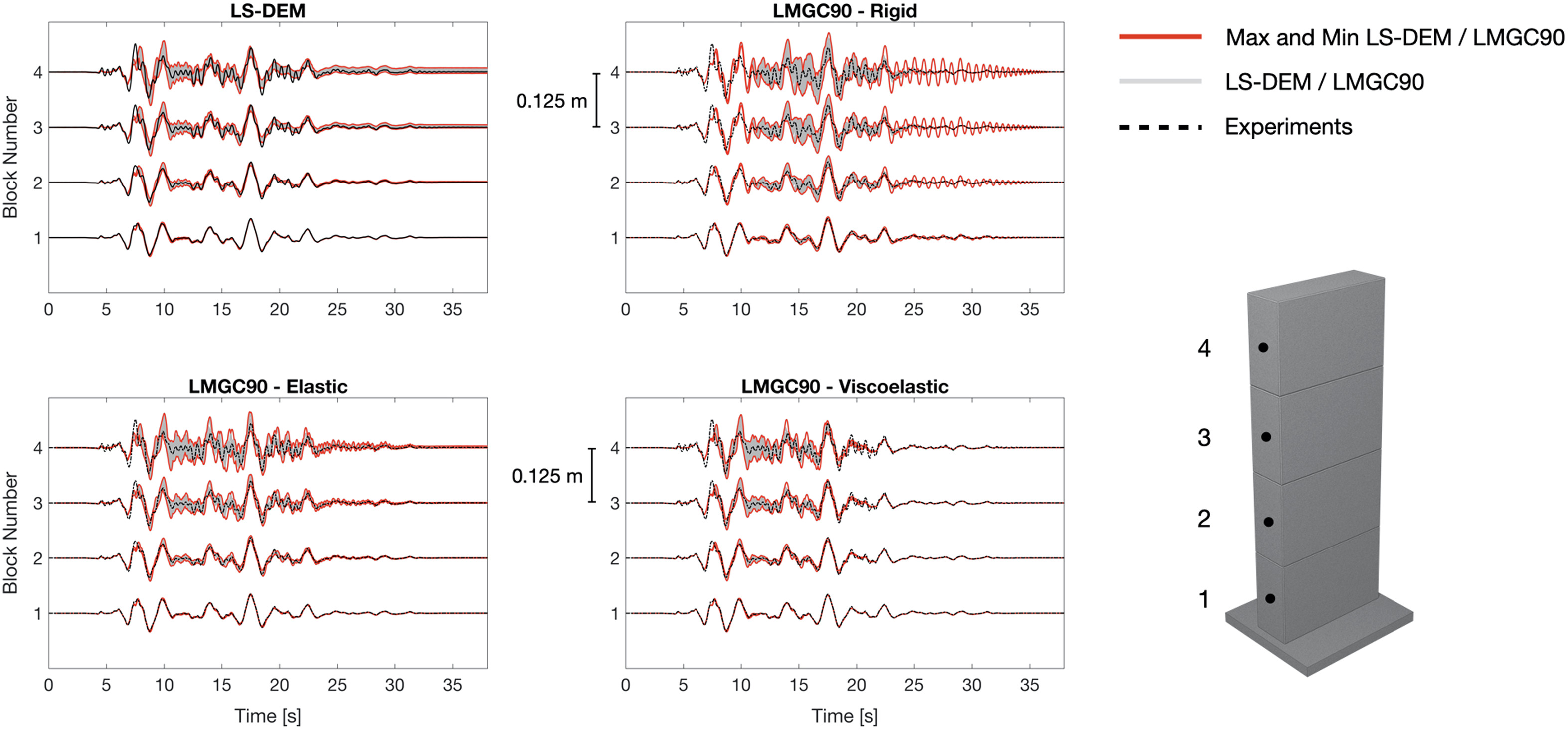
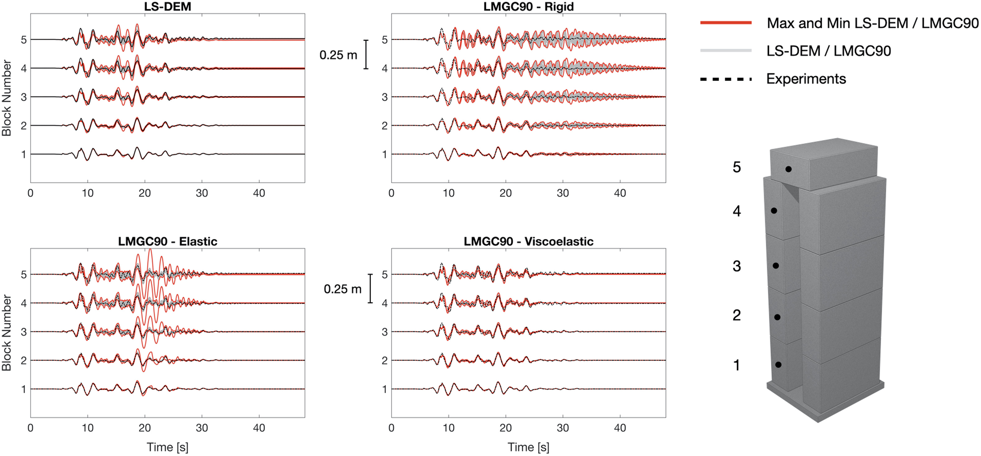
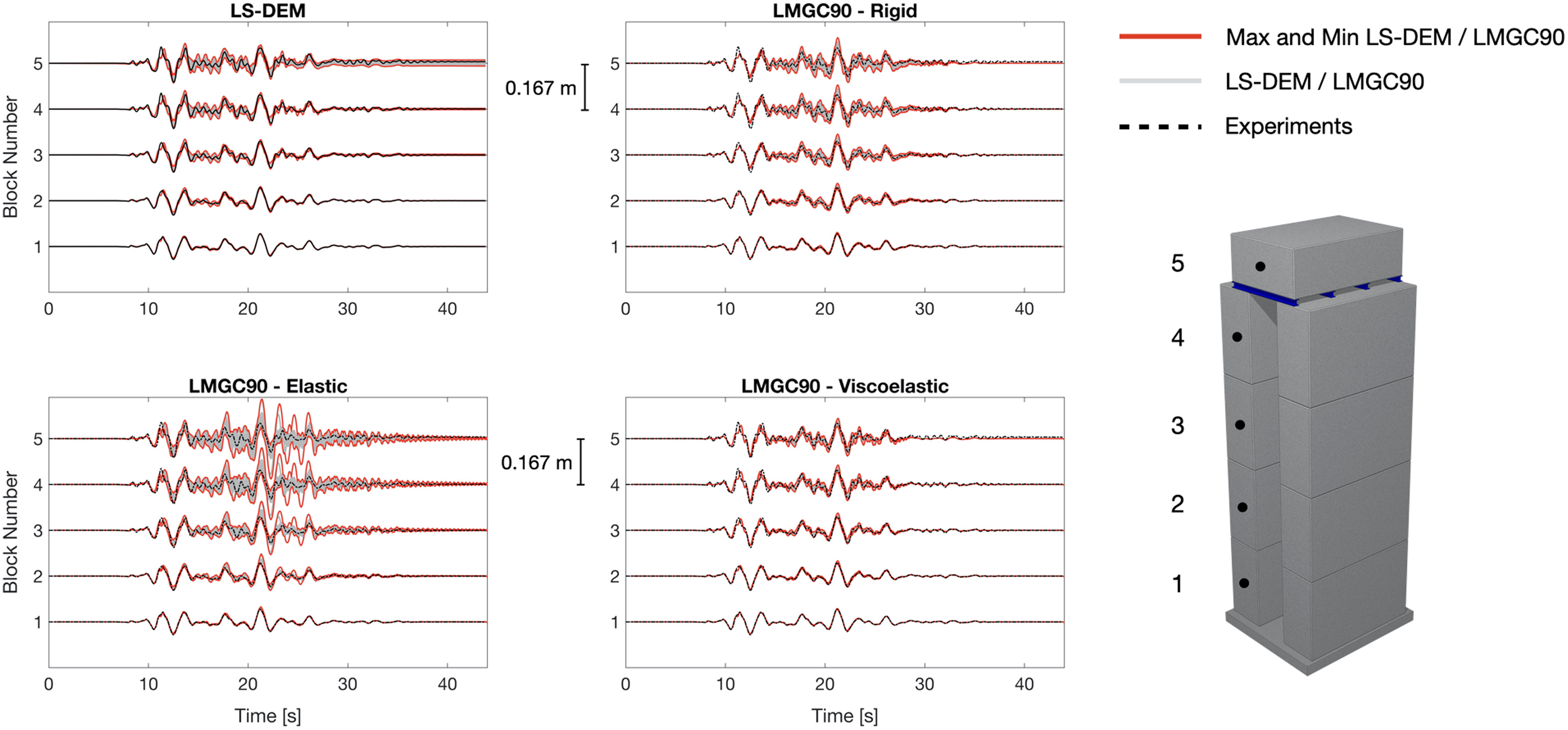
Results are shown in Figs. 11–14. In these figures, the displacement time-history of mass center of the concrete block is plotted against optical readings taken from the face center on the side of the same specimen. The gray shaded area is the overlapping of the lines representing the displacement time-histories of all 50 sample sets, with the red line highlighting the maximum and minimum values along the time axis. The black dashed lines indicate the actual experiment results taken from Eucentre.
LS-DEM Results
In configurations 2, 3, and 4, the displacement envelope of the top block is thicker compared to that of configuration 1. This is inevitable as a result of different model parameters tested. Since kinematics of higher blocks are calculated based on that of the lower ones, as the number of blocks increases, the displacement envelope naturally propagates upward and becomes thicker. Moreover, the onset of rocking or slide-rocking is related to the height-to-width ratio of the assembly (Shenton 1996). Since configuration 1 has the least number of concrete blocks and shortest height, the occurrences of rocking and/or slide-rocking is the fewest among all configurations tested. Configuration 3 and 4 are higher in levels and also are more complicated in structures, so naturally, rocking and/or slide-rocking behavior is more likely to be observed. As those dynamic events happen, the behavior of the blocks can heavily depend on parameters like friction coefficient, density and stiffnesses, thus giving explanation to thicker envelopes for configuration 2, 3 and 4. Similarly, as seen in the LS-DEM result from Fig. 14, the displacement envelope is thicker for the top block compared to that of configuration 3, potentially due to the inclusion of four supporting steel beams.
LMGC90 Results
In LMGC90, three different mechanical behaviors have been analyzed: rigid, elastic, and viscoelastic. The viscoelastic block model described the real seismic behavior of the four configurations the best. The elastic block model described the real behavior in a satisfactory way for configuration 1 and 2. For configuration 3 and 4, the simulated results are not ideal and is showing large deviations between tests due to more complicated concrete structures. The rigid block model behaved satisfactory for all four configurations. Within the same model (rigid, elastic, and viscoelastic), similar responses from LS-DEM were observed: more oscillations and thicker envelope toward more complicated concrete structures.
Comparison and Discussion
Given that the blocks in LS-DEM do not deform, it is natural to compare LS-DEM model with the rigid model of LMGC90. Since the contact surfaces in LS-DEM are viscoelastic due to the presence of springs and dampers, we also included the elastic and viscoelastic behaviors from LMGC90 for references.
From both models, the resemblance between simulation results and experiments is remarkable. Some oscillations and variations in residual displacements can still be observed from certain simulations. However, since the exact values of the input variables from reality are unknown, the experiment data can only be taken as a reference. The stochastic nature of the system is accounted for in the simulations, but the experiment is only one realization of a stochastic system itself. Indeed, the experiments only provided one set of data for each configuration at each earthquake intensity level, while the adopted LHS technique, as any Monte Carlo method, leads to provide multiple realizations for each model at each intensity level.
Given that only absolute displacements are compared, it would be ideal to benchmark the rotational behaviors of the blocks as well. Although such data can be easily extracted from the simulations, rotation angles cannot be easily extracted from the experimental data due to the presence of noise given small block rotations.
Conclusion
The main objective of this study is to validate and benchmark two discrete-system-models (i.e., LS-DEM and LMGC90) against experiments done in Eucentre. After analyzing simulation results from both LS-DEM and LMGC90 calibrated models, we can conclude that the seismic performance coming from LS-DEM is similar to that from LMGC90, and both show remarkable resemblance to the actual experimental result obtained in Eucentre. Given that discrete objects in LS-DEM are rigid with viscoelastic contact, results from rigid model and viscoelastic model of LMGC90 are used for comparison. More rocking and/or sliding is observed from the models for complicated configurations like configuration 3 and 4. Larger deviation in residual displacements is also observed, especially for configuration 4 due to the inclusion of four supporting steel bars. It is important to point out that one experimental result is merely a single realization of a stochastic system. Due to time, resource constraints and the almost impossibility of recreating identical initial samples, it is impractical to repeat the experiments as many times as in the simulations. Conversely, using numerical models as virtual experiments, a large number of realizations can be obtained (using multiple random parameters), generating a wealth of data and deeper insights that are difficult or impossible to obtain experimentally (e.g., force distribution, damage, kinematic fields, etc.). It is apparent that numerical virtual experiments offer a window into stochastic systems such as those studied herein.
Additionally, the paper clearly shows that both numerical models can independently reproduce the experimental results. This finding gives us confidence that, since the experimental results at Eucentre can be replicated accurately, other perhaps more complex configurations can be reproduced. Indeed, the concrete specimens tested in experiments are simplified configurations utilized for benchmarking purposes only. The actual concrete configurations used at CERN for radiation shielding are more complex and involve a much larger number of blocks. Such complex and large systems are impractical for physical modeling. Instead, validated numerical models can and should be deployed to investigate the seismic performance of such complex and large structural systems. Perhaps even more importantly, one can use such validated numerical models to design more seismic resistant concrete assemblies for a variety of purposes.
With the method proposed in (Vořechovský and Novák 2009), one can run Monte Carlo type simulations on discrete systems efficiently to obtain stable estimates with low variability. This paper presented a detailed procedure for tuning the two discrete-system-models for simulating the dynamic response of radiation shielding concrete configurations. However, the same procedure can be replicated for any discrete systems, given user-defined margins and correlation structures. This paper merely presented one family of numerical models for discrete concrete structures, yet the approach is amenable to any other numerical model, thereby proposing a new framework for modeling discrete structural systems.
Data Availability Statement
All models, or code that support the findings of this study are available from the corresponding author upon reasonable request. Some data generated or used during the study, including all experimental data, are proprietary and may only be provided upon request to the European Organization for Nuclear Research.
References
Ambraseys, N., P. Smit, R. Sigbjornsson, P. Suhadolc, and B. Margaris. 2002. “Internet-site for European strong-motion data.” In European commission, research-directorate general, environment and climate programme. Brussels, Belgium: European commission.
Andrade, J. E., A. J. Rosakis, J. P. Conte, J. I. Restrepo, V. Gabuchian, J. M. Harmon, A. Rodriguez, A. Nema, and A. R. Pedretti. 2022. “A framework to assess the seismic performance of multiblock tower structures as gravity energy storage systems.” J. Eng. Mech. 149 (1): 04022085. https://doi.org/10.1061/(ASCE)EM.1943-7889.0002159.
Chatzis, M., and A. Smyth. 2012. “Modeling of the 3D rocking problem.” Int. J. Non-Linear Mech. 47 (4): 85–98. https://doi.org/10.1016/j.ijnonlinmec.2012.02.004.
Chetouane, B., F. Dubois, M. Vinches, and C. Bohatier. 2005. “NSCD discrete element method for modelling masonry structures.” Int. J. Numer. Methods Eng. 64 (1): 65–94. https://doi.org/10.1002/nme.1358.
Cundall, P. 1988. “Formulation of a three-dimensional distinct element model—Part I. A scheme to detect and represent contacts in a system composed of many polyhedral blocks.” Int. J. Rock Mech. Min. Sci. Geomech. Abstr. 25 (3): 107–116. https://doi.org/10.1016/0148-9062(88)92293-0.
de Macedo, R. B., E. Andò, S. Joy, G. Viggiani, R. K. Pal, J. Parker, and J. E. Andrade. 2021. “Unearthing real-time 3D ant tunneling mechanics.” PNAS 118 (36): e2102267118. https://doi.org/10.1073/pnas.2102267118.
Donze, F., V. Richefeu, and S.-A. Magnier. 2009. “Advances in discrete element method applied to soil, rock and concrete mechanics.” Electron. J. Geotech. Eng. 8 (1): 44.
Dubois, F., V. Acary, and M. Jean. 2018. “The contact dynamics method: A nonsmooth story.” C.R. Mec. 346 (3): 247–262. https://doi.org/10.1016/j.crme.2017.12.009.
Harmon, J. M., V. Gabuchian, A. J. Rosakis, J. P. Conte, J. I. Restrepo, A. Rodriguez, A. Nema, A. R. Pedretti, and J. E. Andrade. 2022. “Predicting the seismic behavior of multiblock tower structures using the level set discrete element method.” Earthquake Eng. Struct. Dyn. 52 (9): 2577–2596. https://doi.org/10.1002/eqe.3883.
Harmon, J. M., K. Karapiperis, L. Li, S. Moreland, and J. E. Andrade. 2021. “Modeling connected granular media: Particle bonding within the level set discrete element method.” Comput. Methods Appl. Mech. Eng. 373 (Jan): 113486. https://doi.org/10.1016/j.cma.2020.113486.
Hurmuzlu, Y., and D. B. Marghitu. 1994. “Rigid body collisions of planar kinematic chains with multiple contact points.” Int. J. Rob. Res. 13 (1): 82–92. https://doi.org/10.1177/027836499401300106.
JCSS (Joint Committee on Structural Safety). 2000. JCSS probabilistic model code part 3: Material properties. Deift, Netherlands: JCSS.
JCSS (Joint Committee on Structural Safety). 2001. JCSS probabilistic model code part 2: Load models. Deift, Netherlands: JCSS.
Jean, M. 1999. “The non-smooth contact dynamics method.” Comput. Methods Appl. Mech. Eng. 177 (3): 235–257. https://doi.org/10.1016/S0045-7825(98)00383-1.
Kaplan, M. F. 1989. Concrete radiation shielding: Nuclear physics, concrete properties, design and construction. New York: Wiley.
Karapiperis, K., and J. Andrade. 2021. “Nonlocality in granular complex networks: Linking topology, kinematics and forces.” Extreme Mech. Lett. 42 (Jan): 101041. https://doi.org/10.1016/j.eml.2020.101041.
Kawamoto, R., E. Andò, G. Viggiani, and J. E. Andrade. 2016. “Level set discrete element method for three-dimensional computations with triaxial case study.” J. Mech. Phys. Solids 91 (Jun): 1–13. https://doi.org/10.1016/j.jmps.2016.02.021.
Kawamoto, R., J. Andrade, and T. Matsushima. 2018. “A 3D mechanics-based particle shape index for granular materials.” Mech. Res. Commun. 92 (Sep): 67–73. https://doi.org/10.1016/j.mechrescom.2018.07.002.
Kounadis, A., G. Papadopoulos, and D. Cotsovos. 2012. “Overturning instability of a two-rigid block system under ground excitation.” ZAMM 92 (7): 536–557. https://doi.org/10.1002/zamm.201100095.
Moreau, J. J. 1994. “Some numerical methods in multibody dynamics: Application to granular materials.” Supplement, Eur. J. Mech. A. Solids 13 (4): 93–114.
Shenton, H. W. H. W., III. 1996. “Criteria for initiation of slide, rock, and slide-rock rigid-body modes.” J. Eng. Mech. 122 (7): 690–693. https://doi.org/10.1061/(ASCE)0733-9399(1996)122:7(690).
Sinopoli, A. 1989. “Kinematic approach in the impact problem of rigid bodies.” Supplement, Appl. Mech. Rev. 42 (11S): S233–S244. https://doi.org/10.1115/1.3152395.
Sironi, L., M. Andreini, C. Colloca, M. Poehler, D. Bolognini, F. Dacarro, P. Lestuzzi, F. Dubois, Z. Zhou, and J. E. Andrade. 2023. “Shaking table tests for seismic stability of stacked concrete blocks used for radiation shielding.” Eng. Struct. 283 (May): 115895. https://doi.org/10.1016/j.engstruct.2023.115895.
Stronge, W. J. 1991. “Unraveling paradoxical theories for rigid body collisions.” J. Appl. Mech. 58 (4): 1049–1055. https://doi.org/10.1115/1.2897681.
Swiss Society of Engineers and Architects. 2020. SIA 261—Actions sur les structures porteuses. Jacksonville, FL: SIA.
Tsuji, Y., T. Kawaguchi, and T. Tanaka. 1993. “Discrete particle simulation of two-dimensional fluidized bed.” Powder Technol. 77 (1): 79–87. https://doi.org/10.1016/0032-5910(93)85010-7.
Tu, X., and J. E. Andrade. 2008. “Criteria for static equilibrium in particulate mechanics computations.” Int. J. Numer. Methods Eng. 75 (13): 1581–1606. https://doi.org/10.1002/nme.2322.
Venzal, V., S. Morel, T. Parent, and F. Dubois. 2020. “Frictional cohesive zone model for quasi-brittle fracture: Mixed-mode and coupling between cohesive and frictional behaviors.” Int. J. Solids Struct. 198 (Aug): 17–30. https://doi.org/10.1016/j.ijsolstr.2020.04.023.
Vořechovský, M., and D. Novák. 2009. “Correlation control in small-sample monte carlo type simulations I: A simulated annealing approach.” Probab. Eng. Mech. 24 (3): 452–462. https://doi.org/10.1016/j.probengmech.2009.01.004.
Wang, Y., L. Li, D. Hofmann, J. Andrade, and C. Daraio. 2021. “Structured fabrics with tunable mechanical properties.” Nature 596 (7871): 238–243. https://doi.org/10.1038/s41586-021-03698-7.
Information & Authors
Information
Published In

Journal of Engineering Mechanics
Volume 149 • Issue 12 • December 2023
Copyright
This work is made available under the terms of the Creative Commons Attribution 4.0 International license, https://creativecommons.org/licenses/by/4.0/.
History
Received: Nov 9, 2022
Accepted: May 10, 2023
Published online: Sep 23, 2023
Published in print: Dec 1, 2023
Discussion open until: Feb 23, 2024
ASCE Technical Topics:
- Benchmark
- Business management
- Comparative studies
- Computer models
- Continuum mechanics
- Dynamics (solid mechanics)
- Earthquake engineering
- Engineering fundamentals
- Engineering mechanics
- Geotechnical engineering
- Kinematics
- Kinetics
- Management methods
- Methodology (by type)
- Models (by type)
- Practice and Profession
- Research methods (by type)
- Seismic effects
- Seismic tests
- Solid mechanics
- Structural engineering
- Structural models
- Structural systems
- Tests (by type)
Authors
Metrics & Citations
Metrics
Citations
Download citation
If you have the appropriate software installed, you can download article citation data to the citation manager of your choice. Simply select your manager software from the list below and click Download.