Prediction of Weather-Related Incidents on the Rail Network: Prototype Data Model for Wind-Related Delays in Great Britain
Publication: ASCE-ASME Journal of Risk and Uncertainty in Engineering Systems, Part A: Civil Engineering
Volume 4, Issue 3
Abstract
The impacts of extreme weather events on railway operations are complex and in the most severe cases can cause significant disruption to the rail services, leading to delays for passengers and financial penalties to the industry. This paper presents a prototype data model with logistic regression analysis, which enables exploration of the underlying causal factors impacting on weather-related incidents on the rail network. The methodology is demonstrated by using wind-related delay data gathered from the Anglia Route of Great Britain’s rail network between financial year 2006–2007 and 2014–2015. The work presented draws on a diverse group of data resources, including climatic, geographical, and vegetation data sets, in order to include a wide range of potential contributing factors in the initial analysis. It investigates ways in which these data may be used to predict when and where wind-related disruptions would be likely to occur, thus enabling us to gain a deeper understanding of the conditions that prevail in sites at risk of disruption events, pointing to possible mitigation in the design of the infrastructure, and their relationship to the local environment.
Introduction
Extreme weather conditions, such as high winds, storms, and excessive rainfall, can considerably increase risks of rail system failures, which exert a negative impact on the railway performance (cf. Dept. for Transport 2014). Extreme climatic events lead not only to increased risk of damage to critical railway infrastructure and assets (e.g., tracks and overhead power supplies) but also frequently result in operational delays that propagate through the rail network, causing cascading delays to a succession of train services. As an example, consider the impacts of high winds, which are among the most significant causes of delays on the rail network of Great Britain (GB). Sustained high wind speeds or strong gusts may directly result in effects including excessive swaying of overhead line equipment, especially in areas with long headspans, encroachment of wind-blown debris to the lineside, damage to trees within the railway boundary, or flooding due to blown seawater in coastal sections of line. Indirectly, they may result in delays to train services, damage to pantographs or underslung electrical equipment on vehicles, and even derailments. The standard operational response to high wind speed events defined in the national rulebook for GB’s rail network is for emergency speed restrictions to be applied on sections of the track where high wind speeds are either present or are expected to occur. To help train drivers identify the entry to and exit from these sections, speed limits are normally applied between easily recognizable features, such as stations. This practice frequently results in comparably long sections of track being subject to the restriction, leading to significant delays to services passing through the area. It is critical therefore that the most accurate information possible is used when deciding if a limit is to be applied. This problem may be mitigated in the future by the installation of improved in-cab driver aids, such as in-cab signaling or a connected driver advisory system, which may offer a mechanism by which more location-specific limits could be applied in response to real-time condition information, if live wind speed data could be available (cf. Easton et al. 2014).
In general, operational delays due to extreme weather conditions may occur for many reasons. Obtaining accurate estimations of where and when these incidents will occur, and how much impact they may result in, can depend on a number of local environmental factors in addition to the poor weather itself, such as geographical topology, types of assets and infrastructure present, positioning and alignment of those assets, and a range of ecosystem characteristics (e.g., presence of vegetation, percentage coverage of that vegetation on embankments or cuttings, and resistance of the vegetation present to high winds) within and around the railway boundary. However, the identification of these factors is far from straightforward; even if they could be easily identified, establishing the underlying relationship between the factors and the operational event (e.g., direct causality as opposed to some other indirect or coincidental relationship) and quantifying their impacts on the performance of the railway remain huge challenges. A significant barrier to data-driven operational decision making in this area is in the poor understanding of the complex statistical tools needed to establish and quantify complex relationships in this type of system (cf. Kenn et al. 2017; Moloney et al. 2017). Therefore, work is needed to identify a toolbox of minimally complex statistical tools that control room staff can use to better understand the potential impacts of extreme climatic events when considered alongside other weather and external variables.
Usually, the following three situations may be encountered in assessments of the weather impacts on the rail system. First, an incident could be operationally managed, given that some extreme weather is foreseeable on the basis of monitoring of meteorological variables (e.g., wind speed and temperature) and that it is known that those variables would have met or would be trending toward the predetermined trigger conditions for alerts. In this case, standard operational responses, such as imposition of speed restrictions, canceling, rescheduling, or rerouting the train services would be taken in advance, so as to mitigate the risk of an incident occurring (cf. Rossetti 2007). Second, combined effects of multiple meteorological variables in a given period, be they monitored or not, may result in an impact that causes disruption despite none of the monitored conditions in isolation being serious enough to trigger an alert, for example, the combination of local rainfall with wind (e.g., Brazil et al. 2017). The delays from combinations of the causal factors should still be foreseeable, but their accurate prediction would require careful determination of the relationship between those factors and of the critical threshold values in each case. Third, it is likely that some weather-related delays might not be immediate consequences of either historical or real-time local weather observations. The direct causes in this case may often be foreign interference, such as plastic wastes blown onto the tracks and pantographs. As pointed out by the Weather Resilience and Climate Change Adaptation plans (Network Rail 2014), the primary factor in many wind-related rail incidents often turns out to be the lineside trees. Besides the tree trunks and branches, fallen leaves may otherwise cause adhesion problems (i.e., leaves may cling to damp railheads, releasing natural oils as they are crushed by the wheels of passing vehicles and resulting in wheel slip). To understand the impacts of those effects, it requires us to establish mechanisms by which the monitored weather conditions (via either real-time data or predictions) interrelate with the non-weather-related variables in the system. Any analysis of the root causes of delays attributed to poor weather must involve a wider range of aspects of independent variables (cf. Jaroszweski et al. 2010). In fact, the challenges have long since been highlighted in AEA Technology (2003), which suggested long-term research directions and priorities of GB’s rail industry; follow-up research projects have made substantial contributions toward the delivery of effective adaptations of operational responses to climate changes (see also Rail Safety and Standards Board 2010; Network Rail 2011), such as assessment of temperature-related disruptions (e.g., Dobney et al. 2010; Palin et al. 2013; Ferranti et al. 2016). In the meantime, there have also been results of interests in the wider context of the European railway community, such as the climate adaption schemes from perspectives of the Swedish railways (Lindgren et al. 2009), and the case studies of winter weather impacts on the rail freight network in Finland, Norway, Poland, Sweden, and Switzerland (Ludvigsen and Klæboe 2014). It was noted that the causal relationships between the change in weather conditions and the train service delays might not be easily discoverable, as some general trends relying on simple statistics might not necessarily imply the underlying correlations thereof. Despite numerous studies looking into the intermediate links of the climate monitoring, forecasting of extreme weather conditions, and operational response to climatic effects, work still remains inadequate in terms of investigating the interrelated impact on the performance of the rail system. As far as the existing studies were concerned, explanatory variables considered with respect to the weather-related rail incidents have not been systematically investigated or integrated, and there were deficiencies in analyses of multidimensional features. The room for understanding the impact of extreme weather on the rail system remains to be filled with more in-depth surveys.
This paper aims to identify independent variables that may contribute to weather-related incidents on the rail network in both spatial and temporal contexts, relying on the data integration of historical incident records with local weather observations and lineside vegetation conditions around the locations at the time of known incident occurrences. A pilot study in this was reported in by the authors (Fu and Easton 2016), who performed an empirical analysis of the available data and the feasibility of applying the data-processing techniques. Based on this previous exploration, the work presented in this paper provides a substantial improvement to the methodology. A data model, although still a prototype, is developed to capture key trends in the heterogeneous data, allowing for more reliable predictions of weather-related incidents. The proposed method is then demonstrated in the context of a selected area of GB’s rail network, where it is used to assess the identified factors contributing to wind-related delays, and to predict the likelihood of future delay events occurring in specific locations around the network.
The remainder of the paper is divided into three sections. Further details on the data resources used in the study and on the methods used to clean, integrate, and model the data are presented. How the prototype data model works is then demonstrated with a case study on the GB railway’s Anglia Route. The concluding section summarizes the outcomes of the work and gives specific recommendations for future research based on the proposed methodological framework.
Methodology
Case Study Area
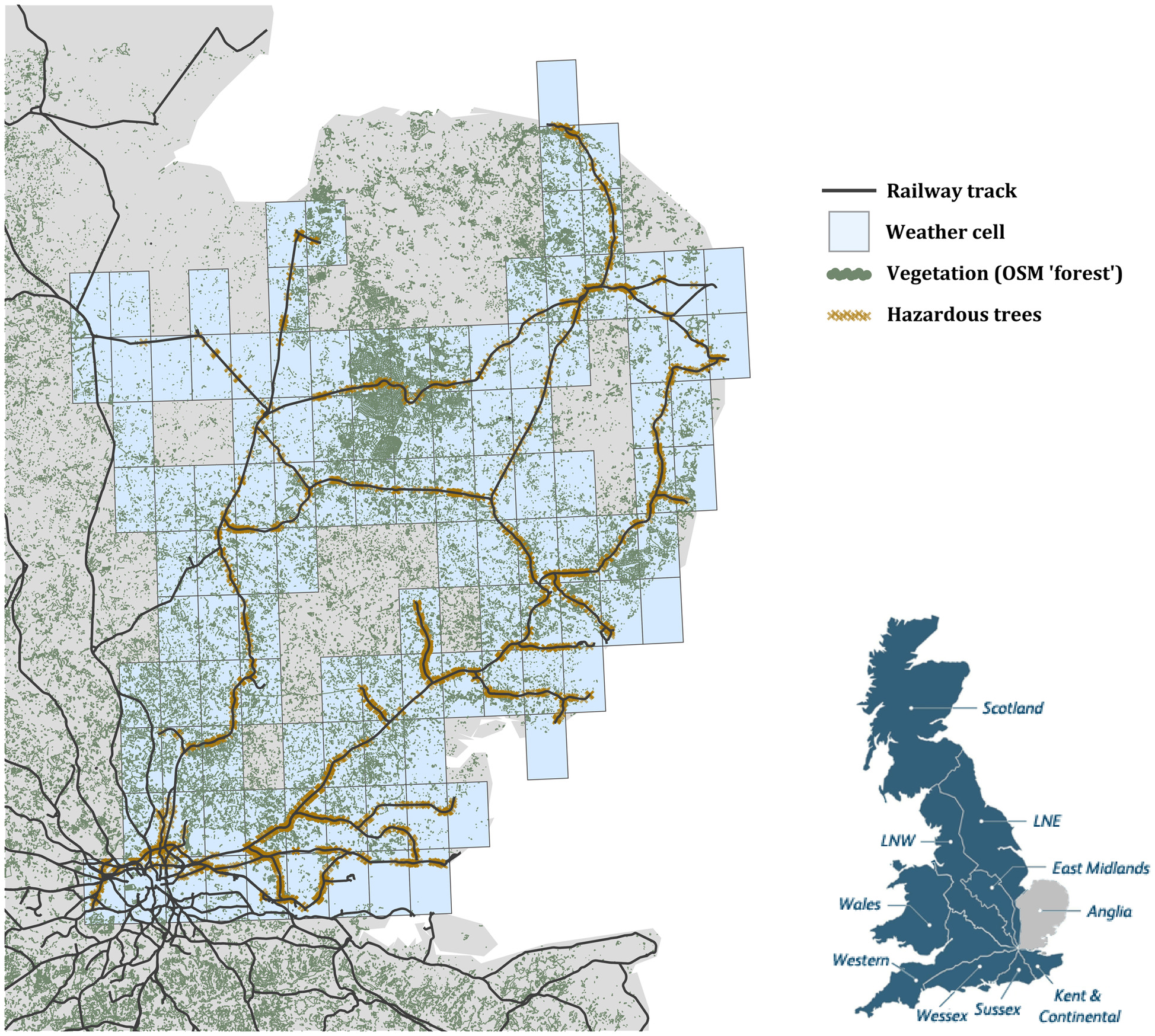
The Anglia Route (hereafter called route), as shown in Fig. 1, is one of the eight strategic geographical routes that form the railway network of GB. It serves a densely populated region in the east of England, which incorporates three strategic route sections, including East Anglia, North London Line, and Thameside. The route includes two main lines: the Great Eastern Main Line and the West Anglia Main Line, along with a number of interurban links, rural routes, and suburban service to the Greater London area. Together these provide both passenger and freight train services across five counties (Network Rail 2016a, b, c). The Route Weather Resilience and Climate Change Adaptation Plans (Network Rail 2014) stated that rail performance on the route had suffered in recent years, mostly as a result of wind-related incidents. In the UK, a financial year runs from April 1 to March 31 of the following year. Beginning in 2006–2007, the economic cost (also called Schedule 8 cost) attributed to wind impacts on the route have accounted for the highest proportion of its delay penalties for weather-related disruptions; by 2014–15, the total annual penalties had reached an average of more than £1 million. Proportionally, around 37.6% of the total weather-related delay minutes were attributed to wind effects, more than twice the value attributed to the second most significant problem—impacts of low adhesion—over the route.
Data Resources
Three main data resources used in the study include details of reported weather-related rail incidents (more specifically, the incidents of delays that were directly attributed to wind), local historical weather observations, and information on the types and extent of lineside vegetation coverage. The three main data sets were all gathered directly from the GB Infrastructure Manager, Network Rail, for the period between financial years 2006–2007 and 2014–2015. In addition, data were gathered from two open data resources: the Railway Codes website (Railway Codes 2017), which includes data on the various coordinate and line reference systems in use in the GB rail industry, and OpenStreetMap (OpenStreetMap Foundation 2017), which is an open-source mapping platform. Each data resource is described in detail in the following subsections.
OpenStreetMap Data
The OpenStreetMap (OSM) provides free access to a wealth of geographical information, including natural topographies, land use, populated settlements, and transport-related objects. Features within a region of interest can be individually extracted as map layers from the OSM database, and these extracts can then be integrated with other data for comprehensive analyses. In the work presented, OSM data were used for visualization purposes. The OSM layers of railways and land use were heavily used. The former was used to show the network of rail lines of the route, and the latter enabled the creation of a visual representation of vegetation coverage over the study area (see also Fig. 1). The vegetation data were used for visual guidance only, and the more detailed records from Network Rail were used in the statistical analysis.
Weather Data
Data of weather observations were made available by Network Rail on an area-by-area basis, with each area called a weather cell and represented in Fig. 1 as a blue rectangle. A weather cell covers an area of the same width and height scaled by geographical coordinates (in degrees of longitude and latitude). The weather cells in the study are at a resolution of 0.125°, as displayed in Fig. 1, and cover all Network Rail infrastructure along the route. The weather data were subject to preprocessing (together with the weather-related incident records) via METEX system, a GIS-based decision support tool used by Network Rail (see also Network Rail 2014). The preprocessed data set kept all records gathered during the study period, involving historical observations of wind and gust speeds (; note that 1.0 mi/h ≈ 1.61 km/h), wind direction (degrees), temperature (°C), and relative humidity (%), each of which was updated hourly. Snowfall (mm) and total precipitation (in millimeter of water equivalent) were also included in the data set, although these were only recorded at intervals of 3 h.
Vegetation Data
Vegetation in and around the lineside area is managed by Network Rail and constitutes part of its assets. Vegetation assets are categorized into several classes. This study focused on vegetation data for two asset classes: vegetation section and hazardous tree, which were collected from a vegetation survey on both sides of the railway track. Traditionally, distance measures used in GB’s rail system are in line with the Imperial system; and is equivalent to 1 furlong (approximately 0.2 km). The vegetation asset class of vegetation section may also be called a furlong vegetation section. The surveys for both vegetation asset classes began in February 2009, and the data were last updated on November 6, 2013, and October 31, 2014, respectively. Data in the furlong vegetation section class were primarily derived via on-site photographs that reflected general characteristics of vegetation for every furlong along railway tracks, such as coverage of various vegetation species, general topography, distance between the vegetation and track, and number of trees. They included information of percentage coverage of 14 vegetation species: alder, ash, beech, birch, conifer, elm, horse chestnut, lime, oak, poplar, shrub, sweet chestnut, sycamore, and willow. In addition, they provided coverage percentages for open space (i.e., exposed areas without trees) and other unspecified features (e.g., bridges and tunnels), along with details on whether the furlong area was electrified. For the hazardous tree class, the condition of individuals was determined by inspection, and summary statistics were generated by geographic location, species, and description. The description included detailed measurements for key attributes (e.g., tree height, diameter, and proximity to railway), but only high-level assessments for others (e.g., the presence of dead wood and whether there was bark congestion and poor foliage). Each asset within the class is assigned a unique identifier, and the identified hazardous trees are presented in Fig. 1.
Weather-Related Incident Data
Delays to scheduled train services on the GB rail network are recorded via the TRUST system—Train Running System on Total Operations Processing System (TOPS)—which monitors vehicle movements across the network. The TRUST data are linked to both the fault management system and control center incident log, enabling detailed information about every rail incident on the network to be derived in terms of date, time, location, observed reason for delay, main actions taken in response to it, and overall resultant delay (min). The data are gathered to enable compensation payments to be made between industry stakeholders in the event of delays; therefore, the calculated total delay values attributed to each incident can be assumed to be reliable (see also Network Rail 2017). Network Rail currently uses nine weather categories to describe incident causes, including adhesion, cold, earth slip, flooding, fog, heat, lightning, snowfall, and wind. Incidents are assigned to one of these categories on the basis of the guidelines in the Delay Attribution Principles and Rules (Delay Attribution Board 2017) and the free-text incident record in the TRUST system. In the study period, more than 2 million incidents were logged in the TRUST database, of which more than 2% had been identified as weather related, although not all the attributions were finalized for the most recent records.
Railway Codification Data
The GB railway network relies on a number of coding methods to describe locations on its infrastructure and to identify the features present (e.g., stations, junctions, and signal boxes). For a typical railway facility (e.g., Aspley Guise railway station), the codification across various systems may be as follows, as described on the Railway Codes website:
The codes BBM and MD140 apply to the route on which Aspley Guise station sits, and APG, 138000, ASPLEYG, and 62051 (ASPLY GSE) apply to the station itself. All of these codes mean different things and are used in different ways.
The complex system of referencing identifiers applied by GB’s railway presents serious technical obstacles to the identification of the same asset of interest across data resource boundaries, but more disturbingly this situation can also arise within a data set, as it is not uncommon for full plaintext names and acronyms to be used arbitrarily by different staff within the same database field. The problems associated with the alignment of data across the resources used in the study required that, as preliminary work, a cross-reference be established allowing easy conversion between systems. The cross-reference was based in large part on manually checked records extracted from the Railway Codes website, a public repository of railway code systems used in UK. The final cross-referencing included coverage of geographical (Cartesian) coordinates, station number names (i.e., STANME), station numbers (i.e., STANOX), timing point locations (i.e., TIPLOCs), engineer’s line references, and track mileages.
Data Processing
Extensive data cleaning and integration was necessary before the raw data sets obtained from Network Rail were suitable for use in the study. Details of these processes can be found in the following sections.
Data Cleansing
Several batch processing tasks were performed to ensure that the data sets were all presented in identical spatial dimensions and formats:
•
Conversion of geographical coordinates between projections in World Geodetic System 1984 and the system used by the Ordnance Survey Great Britain 1936. This was applied to the OSM, weather cells, and vegetation data sets. Such conversion might bring about a bias of up to 5 m; and
•
Conversion of various track mileage data into a consistent format, in terms of both the measurement unit and data type, for the data of incident locations and vegetation assets.
In addition, arrangements were needed to be aligned to the various location codes across the data sets. The GB rail industry normally uses a STANOX code to identify incident locations on the network; however, it is common to also find references that used STANME, TIPLOC, or plaintext names instead. Unfortunately, an official cross-referencing of the data was not available at the time the model was developed. To address this problem, all available information on the full plaintext names for each location was obtained from the Railway Codes website and used to set up a comprehensive cross-referencing repository, which was then used to update the inconsistent location identifiers in the raw data sets and, where practicable, to manually fill in missing STANOX codes given the available plaintext descriptions.
Data Integration
Spatial and Temporal Integration of Weather Data and Incident Records
The weather data associated with each incident were aggregated as follows:
1.
An incident period (IP) was defined, which began a certain number of hours (e.g., 3, 12, or 24 h) before the recorded start time of an incident and lasted until a certain number of hours (e.g., 0, 3, or 6 h) after the recorded end time of the incident. Weather observations during the IP were treated as the prevailing conditions contributing to the incident. The postincident period was included in the analysis, as a subset of the delay events are the result of cancelations to rail services due to knock-on effects from earlier incidents and not as a direct result of the conditions at the time. In this regard, the IP is further divided into two subperiods: a prior IP, which is a subperiod of IP before the recorded start time of an incident; and a posterior IP, which is a subperiod of IP after the recorded end time of an incident.
2.
Next, a corresponding nonincident period (non-IP) was defined for each IP, which began a certain number of hours (e.g., 12, 24, or 36 h) before the IP and lasted until the start of the previously defined IP. In contrast to the IP, the weather conditions observed during the non-IP were assumed to be unlikely to result in a delay incident.
3.
Finally, weather data for the IP and non-IP windows associated with an incident were aggregated based on the weather cell with which the incident location overlapped or, where the incident occurred at a cell boundary, the cell with which the incident location maximally overlapped. Alongside the aggregated data themselves, a set of selected statistics (e.g., mean and maximum) for each of the meteorological variables (e.g., wind and gust speeds) was calculated from the aggregated data for each incident.
A minor complication to the aggregation process exists in the form of incident locations starting in one weather cell but ending in another; in these cases, the most appropriate cell was selected manually. An implicit assumption underpinning this decision was that the prevailing weather conditions would be the same within the scope of an individual weather cell and would not differ significantly between neighboring weather cells in the vicinity of the incident.
Spatial Integration Vegetation Data and Incident Records
As a weather-related delay would likely take place over a wider area than is covered by a single station or section of track, it was necessary to aggregate the vegetation data associated with an incident location in a similar manner to that used for the weather data. Specifically, the vegetation data falling along the length of the track, between the start and end locations of the incident, needed to be included. The only common location identifier shared between the vegetation data set and the incident records were a dyad made up of the engineer’s line reference (ELR) and a track mileage. Usually, the ELRs are used to refer to a specific railway route (e.g., the lower section of the West Coast Main Line), whereas the track mileages relate to the distance measured relative to a major feature on that line (most commonly, a large midpoint or terminal station). In the data analyzed, the recorded starting and ending locations associated with an incident were either within the same route or fall across two or more routes. In the latter cases, the connection point(s) or intermediate route(s) needed to be manually identified, as the information was not recorded in the original data set.
For each recorded incident, the vegetation data were aggregated via the following steps:
1.
All furlong vegetation sections within the incident location were identified (including all relevant railway routes between the start and end places of the incident location);
2.
Data belonging to the two vegetation assets classes (i.e., vegetation coverage and hazardous tree records) were aggregated over the identified furlong vegetation sections; and
3.
Summary statistics were computed over the aggregated data relating to a set of variables, including coverage percentage of open space, proportional coverage of identified species, overall density, total count of trees, average distance of hazardous trees from the track, among others.
Although the vegetation data used in the study were the best available, the vegetation inspections were conducted as independent tasks; that is, the vegetation data were not updated over time with the occurrences of the incidents. As a result, it was likely that the vegetation data presented were not perfectly representative of the trackside conditions at the time the incidents occurred. In developing the data model, the authors assumed that the overall coverage of different species of trees and vegetation did not change much (or remained unchanged) at any given incident location during the study period, and changes in vegetation conditions only took place spatially along the length of the railway section.
Note on the Determination of IP and Non-IP
Regional weather conditions may change constantly during a short period of a day and would be likely to vary significantly from day to day and between day and night. As such, factors contributing to a weather-related delay (e.g., high water level from flooding) may be accumulated over hours or even days prior to the delay event being recorded. Incident duration is also a factor, with records in the incident data provided lasting from anywhere between a few minutes to several days. The selection of appropriate timeframes for the IP and non-IP periods is therefore a critical task in the creation of an accurate predictive model for the weather-related delay events. Existing assessments undertaken by Network Rail specified a single period similar to an IP for analyzing observations of each meteorological variable. For instance, a prior IP of up to 24 h was often considered for analyses of temperature data; however, prior and posterior IPs of 12 h were used for the analyses of wind data. On this account, it would be reasonable to consider an equivalent length for the prior and posterior IPs in this study, although further work in this area will be necessary to look at different combinations of prior IP, posterior IP and non-IP should be assessed on the basis of the type of weather patterns under investigation.
Data Modeling
Logistic Regression
Data modeling activities were performed with the aim of understanding the underlying cause-effect relationships between the prevailing weather conditions, vegetation coverage, and rail service delays and predicting the likelihood of potential future disruptions to rail services occurring, with a secondary aim of giving some indication of the magnitude of those events. Most commonly, regression analysis may be a suitable basis from which researchers might be capable of pursuing all these aims, provided that the delay (and/or the associated delay cost) was considered as a dependent variable (see also McDonald 2009, pp. 207–246). Tentative exploration revealed, however, that the classical regression model, such as multiple regression, might not afford a practical option, as there was no clear evidence indicating that a linear or polynomial relationship between the delay minutes (and/or cost) and the weather or vegetation-related variables existed. In practice, logistic regression has been used extensively as a modeling approach to investigating causes (e.g., weather conditions) for accidents in the transportation field, offering important predictive value on various uncertainties in terms of binary states, such as road traffic accident severity (e.g., Carson and Mannering 2001; Yu and Abdel-Aty 2014), risks of level-crossing accidents (e.g., McCollister and Pflaum 2007), and train derailments (e.g., Schafer 2008). However, few studies have looked at its application in analysis of weather-related incidents on the rail network. For all practical purposes, this study uses a logistic regression model as a prototype, which considers a dichotomous outcome as a dependent variable representing whether a wind-related incident occurred at a particular location. On that basis, a binary classifier could be built on the outcomes at each incident location, enabling the analysis of correlation between the local environment (including weather and vegetation conditions in the immediate vicinity) and the occurrence of delay incidents. It actually evaluates linear relationships between the logarithmic odds of incident occurrence and all explanatory variables (see also Washington et al. 2010, pp. 303–308). In this study, each incident location was associated with a dummy binary variable that took a value of 1 when a wind-related incident occurred at that location, or 0 when no incident was reported at the location. This variable could then be used to assign IP and non-IP windows. The model could be used to predict the probability of the variable taking on the value of 1, which indicates the likelihood of disruptive conditions developing at the associated location. The probabilities would be continuous values ranging from 0 to 1, and a threshold value needs to be set to give the final, binary outcome that was sought. The occurrence of incident can be represented by , and the probability of the incident occurrence , where . Therefore, the model could be specified aswhere = coefficient associated with the th explanatory variable, denoted by ; and = intercept and is associated with a constant 1. With a set of known and data for those explanatory variables , the probability can be calculated by transforming the model specification as
(1)
(2)
As such, the exponential of an estimated coefficient associated with a variable, , which is also known as the odds ratio for the variable , is perceived to be an expected change in the odds of an incident occurring for a unit increase in , given that the other variables remain unchanged (see also Hosmer Jr et al. 2013, pp. 49–86).
Explanatory Variables
Weather-Related Variables
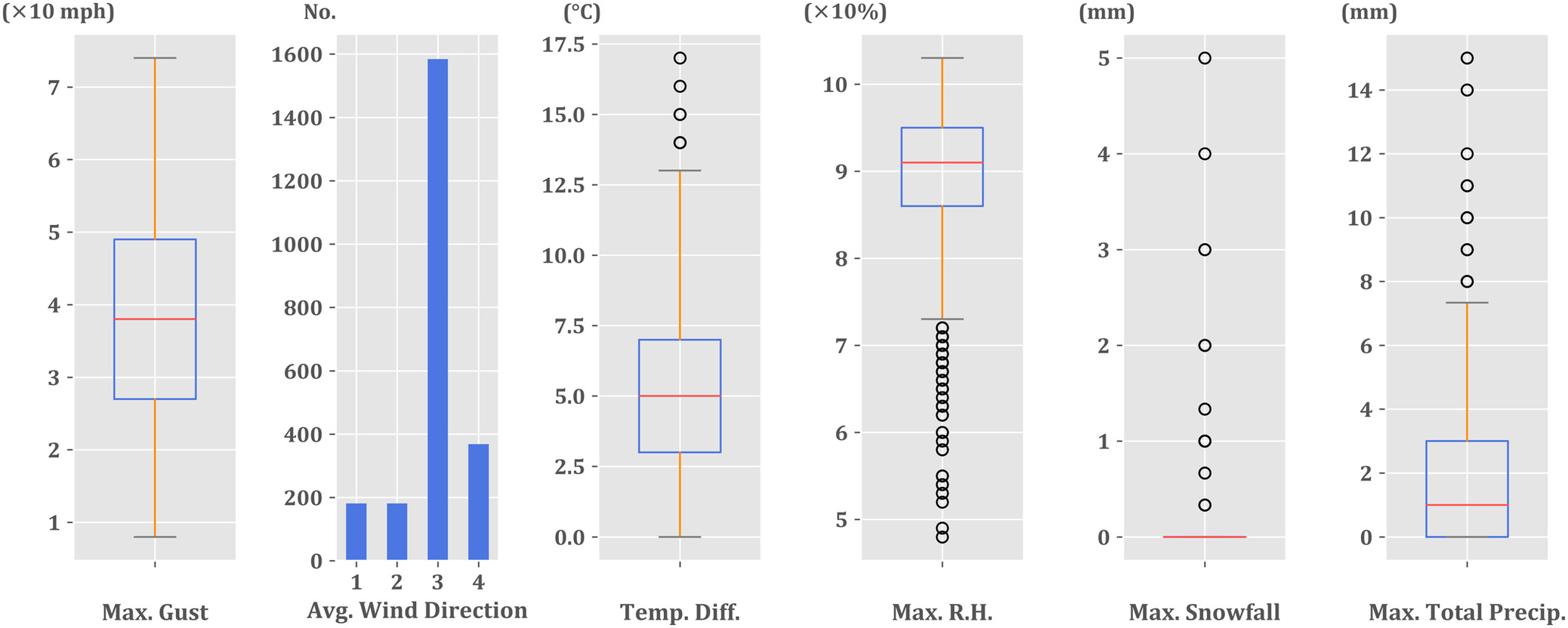
Many of the wind-related incidents in the data set were directly related to the lineside vegetation (e.g., fallen trees blocking the tracks). Although extreme weather conditions (specifically, high wind speeds) would be the most direct cause of the delay event, the root cause may be due to other meteorological variables, such as the temperature and/or relative humidity (RH), which would be precursors to the development of wind-sensitive conditions. The integration process for the weather data included the generation of selected summary statistics for six key meteorological variables: maximum gust speed (; note that 1.0 mi/h ≈ 1.61 km/h); average wind directions categorized into four quadrants as [0°, 90°), [90°, 180°), [180°, 270°), and [270°, 360°); temperature difference between the maximum and minimum (°C); maximum RH (%); total snowfall (mm); and total precipitation (mm). The average wind direction was a categorical variable, so that one of the four directions would need be excluded from model specification.
Vegetation-Related Variables
It has been previously pointed out that timely information of vegetation conditions with respect to the historical weather-related incidents was not available from the available vegetation data set. Therefore, it was assumed that the vegetation conditions of the same incident location were overall unchanged during the study period. This assumption facilitated the data integration. Nevertheless, it was questionable as a generalization in terms of the vegetation coverage over each furlong vegetation section, and it could hardly be tenable in terms of the conditions of hazardous trees for such a long period of time; many might have been removed either before or after incidents. Due to the inherent flaw of the integrated data, it would be highly possible that the effects of different vegetation conditions leading up to incidents might not be effectively captured by any data model. On this account, any variables related to hazardous trees would not be considered; however, it would still be benefitting to conduct a trial for the prototype data model by including the vegetation-related variables such as the coverage percentages of various vegetation species and that of open space and other unspecified features. This might provide us a hint of the roles that those different variables might play leading up to the incidents under different weather conditions. Because the percentage data for each incident location sum to 100, one of the percentage variables would also need to be excluded from the model specification.
In total, 23 explanatory variables were selected for building a prototype data model.
Case Study: Analysis of Wind-Related Delay Events on the Anglia Route
This section demonstrates the application of the previously described methods via a case study of wind-related delay incidents on the Anglia Route of the GB rail network.
Exploratory Analysis
A preliminary visual analysis was firstly performed using high-level summary data, presented as an overlay to the map of the area shown in Fig. 1.
Fig. 2 shows the 15 locations experiencing the most severe wind-related incidents in terms of both severity (i.e., total delay time and compensation payment) and frequency during each financial year of the study; each incident location is marked by a bubble, with colour used to differentiate between financial years. An incident location may be either a single site on the network (e.g., a station) or a route section between any two points. In the latter case, the incident location marked on the map is the midpoint along the track between the start and end locations. The incident locations were added chronologically, so the locations of events from the early years may be completely overlaid by the later ones. As a result, many of the earlier years’ higher-risk locations are not immediately visible. The extent to which the overlapping of events clearly occurs, supports the argument that particular locations along the route could be said to be more prone to disruption or more vulnerable to wind-related delays. With respect to the year-on-year delays and compensation payments, the total delay minutes (as can be seen from the statistics listed next to the color bar) decreased markedly in 2007–2008 to less than a half from 2006–2007. Since then, the total has fluctuated, although overall there was a slight downward trend until 2013–2014. In 2011–2012, the delays attributed to wind reached the lowest level, represented by a total compensation payment of about £0.3 million; however, that figure rose sharply in the following financial year, increasing to more than £4 million. The main reason for that surge in delays is shown in Fig. 3, when an incident at the only location accounting for more than 40,000 delay minutes (approximately 2.8 times that of the second most significant location, London Liverpool Street) occurred at the junction with the East Coast Main Line and caused a huge amount of delay minutes to be accrued. The delay was latter attributed to severe weather beyond the design capability of infrastructure.
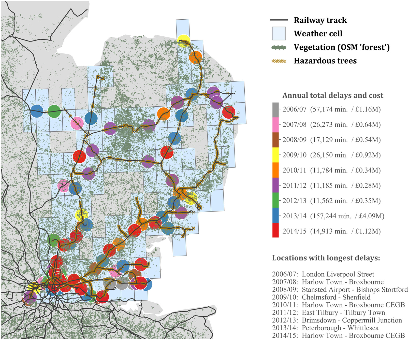
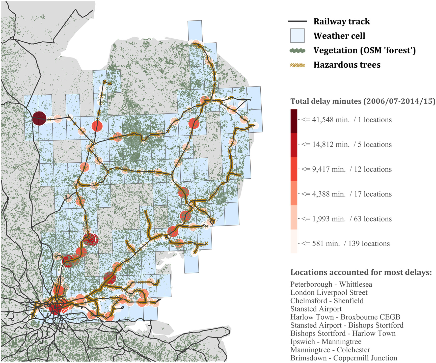
Within the study area, there are a total of 237 incident locations, which are grouped into six severity-based categories using Jenks’ natural breaks (Jenks 1967) in the delay minute data (Fig. 3); the location bubbles are scaled to reflect those categories. A fairly large proportion of the incident occurrences are scattered around the Greater London area and also the neighboring regions to its north and east. To the north of London, a chain of higher-risks locations could be spotted between Stansted Airport and Broxbourne station, passing Bishops Stortford and Harlow Town. More than half of the locations with the highest associated delays listed in Fig. 3 sit within this area and actually lie outside the built-up/industrialized areas of London. In these cases, the rail lines go mainly through a rural landscape (cf. Network Rail 2015), which might suggest a higher likelihood of encountering wind-related incidents if the locations are more exposed to lineside vegetation. Nevertheless, it was unclear from the spatial distributions of incident locations whether dense areas of vegetation cover (of different species) led to an increase in the severity or frequency of wind-related delays, or which other contributing factors might play an active role in the development of the delay incidents over the area. To better understand these issues, a logistic regression model was used to align the data with the approaches discussed in the preceding section. Data related to those extreme incidents, in which the delay minutes were greater than the 99th percentile of the data, were treated as outliers and hence excluded.
Logical Regression Model for Railway Delay Data
Given the exploratory nature of this study, only the basic specification for the logistic regression model was used, which for simplicity does not include any interaction term of explanatory variables (see also the model specification presented in the preceding section).
Derived Data Set
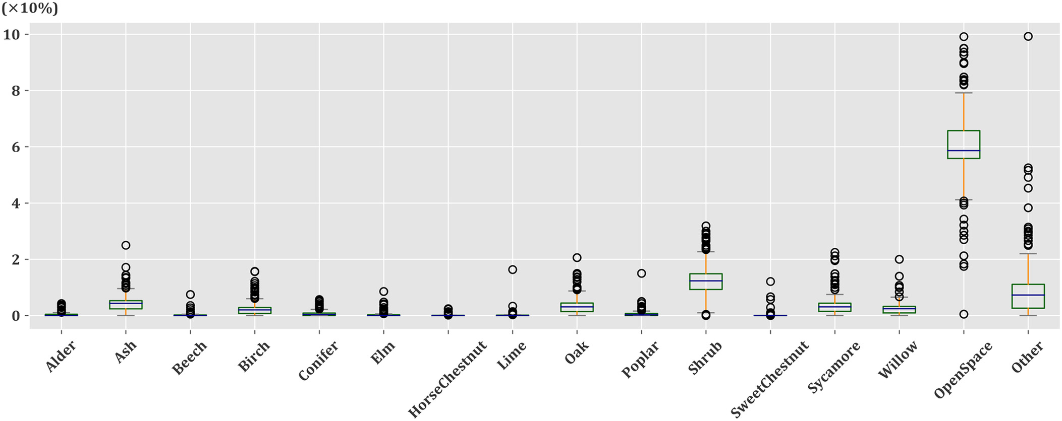
Before the model can be derived, appropriate lengths for the IP and non-IP must be determined. In existing delay attribution studies using weather-related data, Network Rail is known to have used data covering the 12 h of either side of the disruption event. On that basis, the initial model was based around a 12-h prior IP and a 12-h posterior IP; a similar 12-h period was used for the corresponding non-IP. Although the reasoning behind this choice could be considered arbitrary, this allows the results to be directly comparable to those of previous studies and has been observed to produce acceptable results in practice. On the basis of the 12-h periods, a total data set of 2,320 records could be produced from the raw records available. The derived data for the selected weather and vegetation-related variables are described in Figs. 4 and 5, respectively, which illustrate the units and ranges of the data for each variable. Note that for the unit of the maximum gust speed, 1.0 mi/h is equivalent to approximately 1.61 km/h. For the categorical variable, average wind direction, the first to fourth direction quadrants are represented in Fig. 4 by numerals 1–4, respectively.
The derived data set were further split into a training set, containing data between 2006–2007 and 2013–2014, and a test set containing only data from the financial year 2014–2015 (Table 1).
| Data | Financial year | Sample size | ||
|---|---|---|---|---|
| Prior IP = 12 h; posterior IP = 12 h | Non-IP = 12 h | Total | ||
| Training set | 2006–2007 to 2013–2014 | 1,096 | 1,062 | 2,158 |
| Test set | 2014–2015 | 78 | 78 | 156 |
| Derived data set | 2006–2007 to 2014–2015 | 1,174 | 1,140 | 2,314 |
Results
A simple logistic regression model was fitted to the training data set using StatsModels (version 0.8.0), an open-source statistical module implemented in Python environment. The estimated coefficients associated with each variable and the associated significance test results are presented in Table 2.
| Coefficient | Coefficient estimation | Standard error | -value | 95% confidence interval | Odds ratio | |
|---|---|---|---|---|---|---|
| (intercept) | 0.976 | 0.000 | [, ] | — | ||
| 0.9248 | 0.057 | 16.169 | 0.000 | [0.813, 1.037] | 2.521 | |
| 0.289 | 0.001 | [, ] | 0.387 | |||
| 0.223 | 0.000 | [, ] | 0.388 | |||
| 0.245 | 0.106 | [, 0.084] | 0.673 | |||
| 0.6358 | 0.031 | 20.654 | 0.000 | [0.576, 0.696] | 1.889 | |
| 0.9735 | 0.093 | 10.445 | 0.000 | [0.791, 1.156] | 2.647 | |
| 0.3235 | 0.287 | 1.128 | 0.259 | [, 0.886] | 1.382 | |
| 0.033 | 0.273 | [, 0.029] | 0.964 | |||
| 0.0657 | 0.076 | 0.869 | 0.385 | [, 0.214] | 1.068 | |
| 0.1813 | 0.857 | 0.212 | 0.832 | [, 1.860] | 1.199 | |
| 0.1860 | 0.227 | 0.821 | 0.412 | [, 0.630] | 1.204 | |
| 1.182 | 0.242 | [, 0.933] | 0.251 | |||
| 0.304 | 0.469 | [, 0.375] | 0.803 | |||
| 0.1994 | 0.797 | 0.250 | 0.802 | [, 1.761] | 1.221 | |
| 0.9973 | 0.910 | 1.096 | 0.273 | [, 2.780] | 2.711 | |
| 2.333 | 0.466 | [, 2.873] | 0.183 | |||
| 1.189 | 0.512 | [, 1.550] | 0.459 | |||
| 0.0329 | 0.233 | 0.141 | 0.888 | [, 0.490] | 1.033 | |
| 0.563 | 0.291 | [, 0.509] | 0.552 | |||
| 0.119 | 0.697 | [, 0.186] | 0.955 | |||
| 0.8613 | 0.949 | 0.908 | 0.364 | [, 2.721] | 2.366 | |
| 0.2400 | 0.245 | 0.978 | 0.328 | [, 0.721] | 1.271 | |
| 0.269 | 0.343 | [, 0.272] | 0.775 |
Note: .
As Table 2 shows, there was strong statistical evidence at the significance level of 0.05 that all the weather-related variables, except the maximum snowfall and the maximum total precipitation, played positive roles in developing wind-related incidents. The odds ratio for the maximum gust speed was 2.521, which indicates that, in the model, the odds of a wind-related incident occurring would be more than 2.5 times higher with a (approximately 16.1-km/h) increase in the maximum gust speed. The first quadrant of average wind direction (between 0 and 90°) was excluded when fitting the model, so it acted as a reference for assessing effects of the wind directions. For the Anglia Route data, the results show that wind-related incidents are more likely to occur when the average wind direction is within the first quadrant (determined on the basis of the estimates for the other three quadrants all being negative). The odds of an incident occurring can be expected to decrease by more than 60% for wind originating in the opposite quadrant (i.e., between 180 and 270°) or within the second quadrant (i.e., between 90 and 180°). The odds ratio also indicates that a 30% decrease in incident likelihood can be expected when the average wind direction was between 270 and 360°, although this result is less statistically significant.
Alongside the impacts of wind-related effects, some other meteorological variables, such as temperature and relative humidity, also appear to contribute to the risk of wind-related incidents. The temperature difference and maximum relative humidity variables were both found to be statistically positively related to the logarithmic odds of incident occurrences; as such, if all the other variables were fixed to constant values, a 1-unit change in each of these variables could greatly affect the odds of incident occurrence. The reasons for this effect have not yet been fully determined, although work is ongoing.
It is perhaps unsurprising that, overall, the estimated coefficients for the vegetation-related variables were not statistically significant or that their associated -values were too large to prove a connection to the formation of incidents. A possible reason for this is the assumption that the vegetation has not changed significantly with time during the study period, an issue that may be particularly acute in the case of hazardous trees and the IP/non-IP windows surrounding an incident. The large estimate of the intercept may also imply that the effects of the vegetation were not captured by the model. Despite these difficulties, it is possible that the signs of the estimated coefficients may contain some insight into the role different species play in the generation of wind-related delays on the network. Theoretically, any vegetation species with an associated positive coefficient would be more likely to act as a contributing factor to a delay event; that is, in this specific case, an increase of 10% in the coverage of such species would increase the odds of a delay occurring, provided that all other variables (including the weather-related variables) remained constant. According to surveys undertaken by Duryea et al. (2007a, b), many conifers, ash, and elm have relatively low wind resistance. Similarly, species such as sycamore are typical examples of trees with a low modulus of rupture—they break easily under bending and hence have low survival rates. Some tree species, such as live oak and laurel oak, may show a relatively higher modulus of rupture, which means that they would be less likely to fall during strong winds; however, they may also lose branches, which in turn could result in an operational delay. In the Anglia Route data, the estimated coefficients associated with all these species mentioned were found to be positive, supporting these theories. The effects of any increase in these variables would be conditional on a corresponding decrease in the open space coverage. However, given the Anglia Route data, there was no statistical evidence suggesting that species coverage was significantly related to the odds of incident occurrences. Gaining a deeper insight into these issues would be of value to the industry; however, this is out of the scope of the study.
Use of the Trained Model in the Prediction of Delay Events
To test the predictive abilities of the model, the test data set that was held back during training was used as a basis for performance assessment. Fig. 6 shows the receiver operator characteristic (ROC) plot, where the area under the ROC curve (AUC) could be used as a measure of quality of classification models. In general, a model would be considered to perform well when the AUC is greater than 0.8.
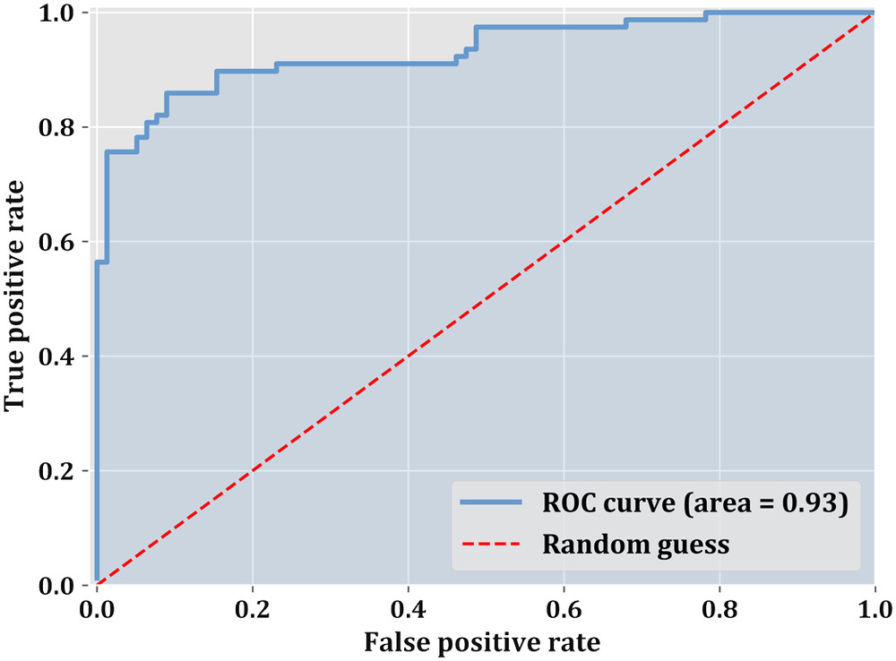
When used to predict the occurrence of wind-related incidents, the model presented in this study had an AUC of 0.93 (Fig. 6), demonstrating excellent performance against the real data in the test set. Used alongside the ROC, the true positive rate (TPR) (also known as sensitivity) for a classifier indicates the probability of the binary outcome variable taking the value of 1 when a wind-related incident actually occurred. In contrast, the false positive rate (FPR) (also known as 1-specificity) indicates the probability of the outcome variable taking the value of 1 while in fact there was no incident reported. Put simply, the TPR represents the proportion of the actual incidents that were correctly predicted by the classifier among the cases labeled 1, whereas the proportion of the non-incident cases that were correctly identified among all labeled 0 should be equal to FPR subtracted from 1. To achieve acceptably high TPRs and low FPRs, it is necessary to fine-tune the threshold value used in the binary classification. The most common way of determining the optimal threshold is to maximize the sum of sensitivity and specificity (Greiner et al. 2000); using this approach, the threshold value for the data in the current case was approximately 0.52.
Fig. 7 shows the predicted delay events and their associated probabilities, alongside the threshold value used in the binary classifier (prior IP, posterior IP, and non-IP in this case were all set to be 12 h).
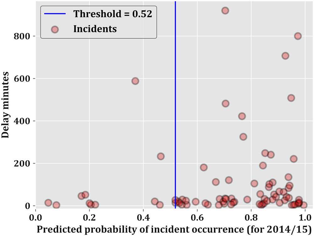
Where the associated test data contained events with a significant operational delay (total delay to services greater than 200 min), nearly all of these are contained within the group above the threshold value, and indeed most have predicted probabilities in excess of 0.7. However, one significant outlier, which led to nearly 600 min of delay, did exist as it was only predicted with a probability of around 0.4, far too low for selection at the proposed threshold. The reason for the poor performance in this case was not clear.
Conclusions
In this paper the authors have presented a rudimentary framework for integrating and modeling of climate-related delay data on the GB rail network. The work aimed to develop a deeper understanding of the relationship between the occurrences of delay incidents and a range of variables associated with the local environments. The data used in the study were drawn from a variety of sources, including historical incident reports, weather observations, and surveys of the types and coverage rates of lineside vegetation. A selection of variables from the integrated data set was used to fit a logistic regression model against delay data recorded on the Anglia Route of Great Britain’s railway network. The initial results from the prototype data model have demonstrated good overall performance in terms of both sensitivity and specificity of the delay predictions. In addition to the expected contributing factors (e.g., high-speed wind/gust), the model identified a number of other weather-related variables, such as wind direction, relative humidity, and temperature variations as indicative of an increasing risk of wind-related delay incidents occurring.
Data relating to lineside vegetation were not found to contribute in a statistically significant way to the prediction of delays; however, the authors believe that issues around the timeliness of these data and assumptions that the vegetation has not changed significantly during the periods of interest immediately surrounding an incident are likely problematic, and further work is needed in this area.
Although this study has focused on wind-related delay events, the prototype data model is sufficiently generic that it should be easily adaptable to the analysis of rail incidents attributed to other categories of weather events, including those related to extremes of temperature, adhesion incidents, and flooding. However, if the model were to be used in support of these use cases, it is likely that further variables external to the current data set may need to be considered.
Certainly, further work is needed for the prototype data model being generalized to a larger scale and wider contexts. From a pragmatic view, the predicted probability of incident occurrences should indicate whether a given rail subnetwork would be more sensitive or more likely to suffer higher risk to high-wind events at a certain period. More specifically, given the data of a location and a period, if a predicted probability is above a threshold value, it would be assumed that an incident would occur around the location and the time. In this regard, determining the threshold value is a matter of expert interpretation. Also, it would be recommended that further inspections may be necessary, especially where the predicted probabilities were lower than the threshold while incident did actually occur. Any statement and/or assumption on this should be largely supported and/or verified by statistical evidence via both the industry and the established data modeling framework. In another aspect, there appeared to be an arbitrary relationship between the actual delay minutes and predicted probabilities from the prototype data model. However, given more information and/or variations in the model specification, it remains unclear whether the incident magnitude in terms of the length and economic cost of the delays could also be captured and reflected by improved data models.
Looking to the future, the work has shown that there is an outstanding issue in the GB rail industry around the diverse set of coding systems for location information currently in use on the network; this issue posed a major obstacle to effective data integration in the study. Development of interoperable data links or a publicly accessible reference database in this area would be highly beneficial to the wider industry.
The process for defining/determining incident and nonincident periods (i.e., IPs and non-IPs) used in the study was drawn directly for similar work performed in the past, and although it has proven effective, further development is needed in this area before a rigorous, repeatable process exists that can be used across studies in different domains. The analysis and results presented in this paper may provide some guidance on this matter; however, further consultation with industrial experts will be vital to the success of such work going forward.
The vegetation data used in this study were effectively a single snapshot that was likely not sufficiently representative of the real-world conditions at the time of delay incidents occurring to serve as a firm basis for model generation. Updated automated survey techniques may soon be able to provide much more frequent estimations of the coverage and condition of various species along the boundaries of the railways; until such data becomes available, it may not be possible to generate models of the type proposed in this study that take account of vegetation-related data at incident locations.
Finally, there is significant scope remaining for improvements in the modeling techniques used, particularly in model specification. The authors believe that specific research effort should be devoted to (1) specifying different IPs for the various weather-related variables; (2) including provision for interactions between variables within the model; (3) including external factors influencing the scale of the delays, such as geographical topology and line utilization; and (4) accounting for latent classes with respect to specific incident reasons and different seasons. Moreover, an ongoing live calibration of the model produced against live weather data feeds and the associated network delays would enable a more detailed estimation of future performance and hopefully increase confidence in the results.
Acknowledgments
This study was funded by Network Rail as part of their strategic partnership in data integration and management with the University of Birmingham. The authors thank Network Rail for their continued support, particularly Caroline Lowe, Steve McCulloch, and Ron Sutherland.
References
AEA Technology. 2003. Safety implications of weather, climate and climate change., London: Rail Safety and Standards Board.
Brazil, W., A. White, M. Nogal, B. Caulfield, A. O’Connor, and C. Morton. 2017. “Weather and rail delays: Analysis of metropolitan rail in Dublin.” J. Transp. Geogr. 59 (Feb): 69–76. https://doi.org/10.1016/j.jtrangeo.2017.01.008.
Carson, J., and F. Mannering. 2001. “The effect of ice warning signs on ice-accident frequencies and severities.” Accid. Anal. Prev. 33 (1): 99–109. https://doi.org/10.1016/S0001-4575(00)00020-8.
Delay Attribution Board. 2017. Delay attribution principles and rules. London: Delay Attribution Board.
Dept. for Transport. 2014. Government response to the transport resilience review. : Dept. for Transport.
Dobney, K., C. J. Baker, L. Chapman, and A. D. Quinn. 2010. “The future cost to the United Kingdom’s railway network of heat-related delays and buckles caused by the predicted increase in high summer temperatures owing to climate change.” Proc. Inst. Mech. Eng., Part F: J. Rail Rapid Trans. 224 (1): 25–34. https://doi.org/10.1243/09544097JRRT292.
Duryea, M. L., E. Kampf, and R. C. Littell. 2007a. “Hurricanes and the urban forest: I. Effects on southeastern United States coastal plain tree species.” Arboriculture Urban For. 33 (2): 83–97.
Duryea, M. L., E. Kampf, R. C. Littell, and C. D. Rodriguez-Pedraza. 2007b. “Hurricanes and the urban forest: II. Effects on tropical and subtropical tree species.” Arboriculture Urban For. 33 (2): 98–112.
Easton, J. M., D. Jaroszweski, A. Quinn, L. Chapman, and C. Baker. 2014. The assessment of anemometer based wind alert systems for implementation in GB: Operational context and requirements. London: Rail Safety and Standards Board.
Ferranti, E., L. Chapman, C. Lowe, S. McCulloch, D. Jaroszweski, and A. Quinn. 2016. “Heat-related failures on southeast England’s railway network: Insights and implications for heat risk management.” Weather Clim. Soc. 8 (2): 177–191. https://doi.org/10.1175/WCAS-D-15-0068.1.
Fu, Q., and J. M. Easton. 2016. “How does existing data improve decision making? A case study of wind-related incidents on rail network.” In Proc., Int. Conf. on Railway Engineering (ICRE 2016), 1–7. Brussels, Belgium: Institution of Engineering and Technology.
Greiner, M., D. Pfeiffer, and R. D. Smith. 2000. “Principles and practical application of the receiver-operating characteristic analysis for diagnostic tests.” Preventive Vet. Med. 45 (1–2): 23–41. https://doi.org/10.1016/S0167-5877(00)00115-X.
Hosmer, D. W. Jr, S. Lemeshow, and R. X. Sturdivant. 2013. Applied logistic regression. New York: Wiley.
Jaroszweski, D., L. Chapman, and J. Petts. 2010. “Assessing the potential impact of climate change on transportation: The need for an interdisciplinary approach.” J. Transp. Geogr. 18 (2): 331–335. https://doi.org/10.1016/j.jtrangeo.2009.07.005.
Jenks, G. F. 1967. “The data model concept in statistical mapping.” Vol. 7 of International yearbook of cartography, edited by K. Frenzel, 186–190. London: George Philip & Son.
Kenn, G., A. Dane, and K. Giles. 2017. “Network Rail: A new approach to coastal asset management— North Wales case study.” Infrastruct. Asset Manage. 4 (1): 8–18. https://doi.org/10.1680/jinam.15.00013.
Lindgren, J., D. K. Jonsson, and A. Carlsson-Kanyama. 2009. “Climate adaptation of railways: Lessons from Sweden.” Eur. J. Transp. Infrastruct. Res. 9 (2): 164–181.
Ludvigsen, J., and R. Klæboe. 2014. “Extreme weather impacts on freight railways in Europe.” Nat. Hazards 70 (1): 767–787. https://doi.org/10.1007/s11069-013-0851-3.
McCollister, G. M., and C. C. Pflaum. 2007. “A model to predict the probability of highway rail crossing accidents.” Proc. Inst. Mech. Eng. Part F: J. Rail Rapid Trans. 221 (3): 321–329. https://doi.org/10.1243/09544097JRRT84.
McDonald, J. H. 2009. Handbook of biological statistics. Baltimore: Sparky House.
Moloney, M., T. McKenna, K. Fitzgibbon, and E. McKeogh. 2017. “Quality data for strategic infrastructure decisions in Ireland.” Infrastruct. Asset Manage. 4 (2): 40–49. https://doi.org/10.1680/jinam.16.00011.
Network Rail. 2011. “Operations and management: Adapting to extreme climate change (TRaCCA), Phase 3 Report—Tomorrow’s railway and climate change adaptation.”. London: RSSB and Network Rail.
Network Rail. 2014. “Route Weather Resilience and Climate Change Adaptation (WRCCA) plans: Anglia.” WRCCA plans. London: Network Rail.
Network Rail. 2015. Route specifications: Anglia. London: Network Rail.
Network Rail. 2016a. “Anglia Route study.” Long term planning process, London: Network Rail.
Network Rail. 2016b. “Network specification 2016: Anglia.” Long-term planning, London: Network Rail.
Network Rail. 2016c. Route specifications 2016: Anglia. London: Network Rail.
Network Rail. 2017. “Payments for disruption on the railway.” Accessed August 1, 2017. http://archive.nr.co.uk/payments-for-disruption-on-the-railway/.
OpenStreetMap Foundation. 2017. “OpenStreetMap.” Accessed June 6, 2017. https://www.openstreetmap.org.
Palin, E. J., H. E. Thornton, C. T. Mathison, R. E. McCarthy, R. T. Clark, and J. Dora. 2013. “Future projections of temperature-related climate change impacts on the railway network of Great Britain.” Clim. Change 120 (1): 71–93. https://doi.org/10.1007/s10584-013-0810-8.
Rail Safety and Standards Board. 2010. Tomorrow’s railway and climate change adaptation: Phase 1 Report (T925 Report). RSSB Managed Cross-Industry Research Project. London: Rail Safety and Standards Board.
Railway Codes. 2017. “Railway codes and other data.” Accessed June 6, 2017. http://www.railwaycodes.org.uk.
Rossetti, M. A. 2007. “Analysis of weather events on U.S. railroads.” In Proc., 23rd Conf. on Interactive Information Processing Systems (IIPS). Boston: American Meteorological Society.
Schafer, D. H. 2008. “Effect of train length on railroad accidents and a quantitative analysis of factors affecting broken rails.” M.Sc. dissertation, Dept. of Civil and Environmental Engineering, Univ. of Illinois at Urbana-Champaign, Urbana, IL.
Washington, S. P., M. G. Karlaftis, and F. L. Mannering 2010. Statistical and econometric methods for transportation data analysis. Boca Raton, FL: CRC Press.
Yu, R., and M. Abdel-Aty. 2014. “Using hierarchical Bayesian binary probit models to analyze crash injury severity on high speed facilities with real-time traffic data.” Accid. Anal. Prev. 62 (Jan): 161–167. https://doi.org/10.1016/j.aap.2013.08.009.
Information & Authors
Information
Published In

ASCE-ASME Journal of Risk and Uncertainty in Engineering Systems, Part A: Civil Engineering
Volume 4 • Issue 3 • September 2018
Copyright
This work is made available under the terms of the Creative Commons Attribution 4.0 International license, http://creativecommons.org/licenses/by/4.0/.
History
Received: Aug 7, 2017
Accepted: Mar 2, 2018
Published online: Jun 19, 2018
Published in print: Sep 1, 2018
Discussion open until: Nov 19, 2018
Authors
Metrics & Citations
Metrics
Citations
Download citation
If you have the appropriate software installed, you can download article citation data to the citation manager of your choice. Simply select your manager software from the list below and click Download.