Simulating Multihazard Interactions Using Higher-Order Network Analysis
Abstract
Our built environment is often subjected to multiple (natural) hazards’ concurrent and/or sequential impacts. Modeling multihazard interactions (i.e., possible interrelationships between hazard events with their associated frequencies and severities and resulting impacts on a specific location or region of interest) and simulating multihazard scenarios (or event sets; i.e., realizations of possible multihazard interactions) to design and assess civil infrastructure is crucial. This paper presents a probabilistic framework for simulating multihazard scenarios, aiding in civil infrastructure design and risk assessment. Specifically, the proposed approach leverages temporal hypergraphs for characterizing the hazard interactions. Temporal hypergraphs are a higher dimensional generalization of a graph that can capture multi-way connections (i.e., not just pairwise) that can change over time. The temporal attributes of the hypergraphs are defined using a series of occurrence models and simulation-based approaches to generate the arrival times and features (e.g., event characteristics and local intensities) of all considered hazards over a defined space-time interval. A sliding window procedure is also proposed to support decision-makers and other end users in identifying critical multihazard scenario windows that can significantly impact the resilience of the built environment. The framework’s applicability is demonstrated using an illustrative example of a hypothetical region susceptible to earthquake-induced ground shaking, liquefaction, tsunami, and riverine flooding. The proposed framework can help decision-makers design and test efficient disaster risk mitigation and management policies. Furthermore, the proposed multihazard scenario modeling framework can be combined with vulnerability/impact assessment methodologies to quantify the multihazard risk of exposed infrastructure and communities.
Introduction
Recent disasters globally [e.g., the 2018 Central Sulawesi, Indonesia, earthquake, tsunami, and liquefaction (Cilia et al. 2021); the 2010/2011 Christchurch, New Zealand, earthquake sequence and liquefaction (Green et al. 2014); and the 2011 Tohoku, Japan, earthquake and tsunami (Mori and Takahashi 2012)] have highlighted the susceptibility of our built environment to the concurrent and sequential impacts of multiple natural hazards during their service life. Decision-makers now face the challenge of developing disaster risk management plans/strategies for multiple hazards and considering the impacts of possible hazard interactions. The term hazard interaction is defined as possible interrelationships between hazard events with their associated frequencies and severities and resulting impacts on a specific location or region of interest.
Due to the complexity of identifying, modeling, and characterizing hazard interactions, most research efforts in multihazard risk assessment have often focused on qualitative and semi-quantitative approaches. Qualitative methods (e.g., Gill et al. 2020; Pescaroli and Alexander 2018) typically focus on descriptive and/or anecdotal methodologies to illustrate relationships and dependencies between primary and secondary hazards, their characteristics, and potential impacts. Semi-quantitative approaches (e.g., Greiving et al. 2006; El Morjani et al. 2007; Schmidt-Thomé et al. 2006) typically adopt weighting methods to develop indices for quantifying multihazard risk. Such qualitative and semi-quantitative methods provide good comparative insights into multihazard risks, which is especially helpful for identifying multihazard risk hotspots and risk-reduction prioritization exercises (e.g., Sevieri et al. 2020). Nevertheless, the absence of robust quantitative techniques to simulate hazard interactions (and their impacts) makes the application of these qualitative and semi-quantitative approaches in probabilistic risk assessment frameworks (e.g., performance-based engineering design and assessment frameworks) difficult.
In recent years, more research has been devoted to quantifying multihazard interactions. For example, studies (e.g., Ming et al. 2022; Petroliagkis et al. 2016; Svensson and Jones 2002; Zellou and Rahali 2019; Zheng et al. 2014) have developed quantitative multihazard analysis and risk assessment frameworks for compound flooding considering hazard interactions. Studies (e.g., Johansson et al. 2015; Qie and Rong 2022; Zuccaro et al. 2018) have proposed frameworks for cascading hazard scenario analysis. Furthermore, other studies (e.g., Decò and Frangopol 2011; Kameshwar and Padgett 2014; Li et al. 2020; Nguyen Sinh et al. 2016; Rosowsky and Wang 2012) have proposed various approaches to capture the joint occurrence of independent hazards.
A major drawback of current quantitative approaches is their limited scope, which fails to capture all potential hazard interactions. Furthermore, some existing studies adopt a multi-layer, single-hazard approach in which each hazard is considered in isolation before all resulting impacts are combined. As Gill and Malamud (2014) discussed, the multi-layer, single-hazard approach may result in risk underestimation, potentially impacting decision-making for effective multihazard risk reduction and management. Therefore, developing an effective holistic multihazard simulation tool that efficiently captures possible hazard interactions and provides sufficient information for end users and various stakeholders to make relevant, risk-informed decisions for civil infrastructure is essential.
This paper seeks to advance the field of multihazard risk assessment by developing a probabilistic multihazard scenario simulation framework that accounts for hazard interactions in a given region of interest. Specifically, we adopt the temporal hypergraph theory to characterize possible hazard interactions over time and space. The framework’s applicability is demonstrated using an illustrative example of a hypothetical region impacted by multiple natural hazards with realistic assumptions for each hazard modeling/characterization and their dependencies.
Proposed Framework
Overview
Multihazard risk analysis requires appropriate consideration of two levels of interactions—Level I (or direct) and Level II (or indirect) interactions (Zaghi et al. 2016). Level I interactions occur due to the inherent interrelationships of hazards and are independent of the presence of physical components. Level II interactions look at hazard interrelationships through site effects and impacts on physical components, systems, and networks (e.g., flood occurrence due to the earthquake-induced collapse of a dam or pipelines, wildfire occurrence from earthquake-induced damage to gas refineries, or landslide occurrence due to the earthquake-induced collapse of a retaining structure). The framework presented in this study focuses only on Level I interactions. Future studies will explore extending the methodology to consider Level II interactions.
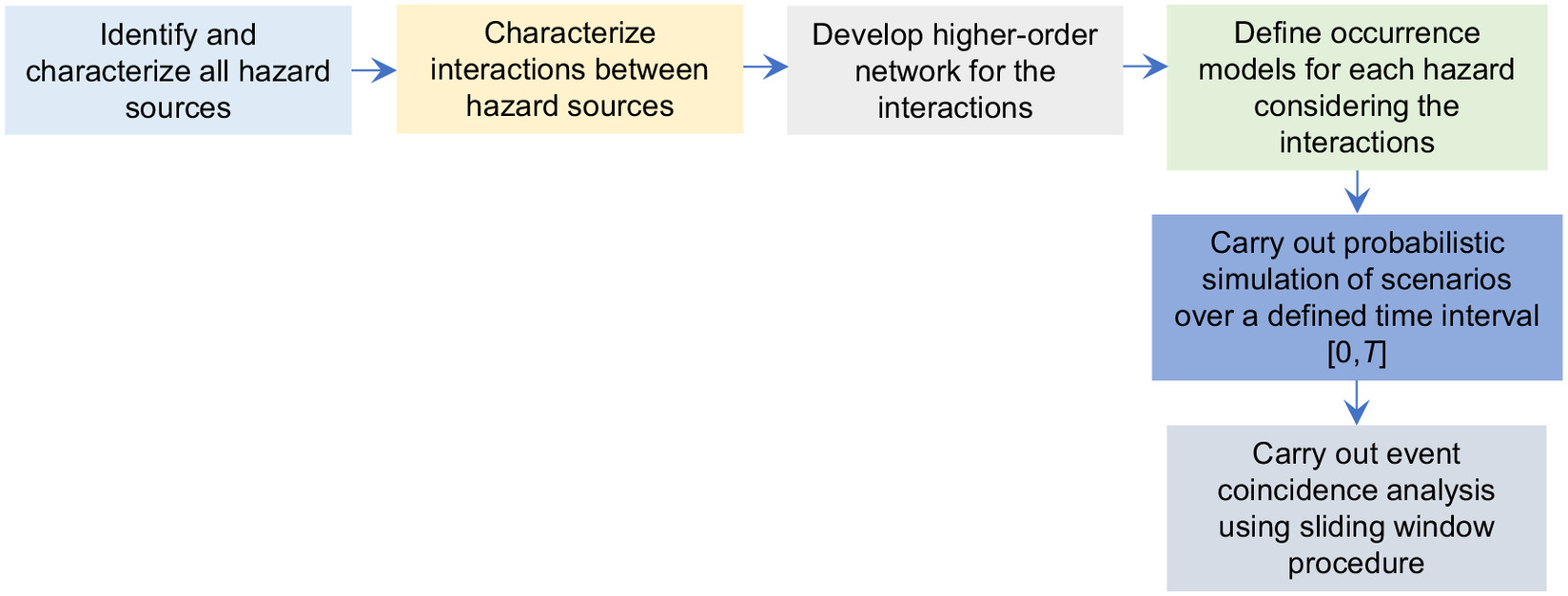
Appropriate multihazard analysis of Level I interactions entails identifying all potential hazard sources in a geographical region of interest, defining and characterizing their potential interactions, defining relevant occurrence models for each hazard considering such interactions, and probabilistically simulating multihazard scenarios over a defined space-time domain. In this study, hazard sources collectively refer to various phenomena (natural or human-induced) that result in events that can potentially lead to disasters. Sometimes, these hazard sources are physically tied to specific locations. For example, earthquakes are linked to geological faults, and riverine flooding is associated with rivers. A flowchart for multihazard analysis capturing the steps mentioned previously is presented in Fig. 1. The subsequent subsections provide a detailed description of each step.
Identifying Hazard Sources and Characterizing Their Potential Interactions
Hazard analysis characterizes the occurrence time, location, severity, spatial and temporal scales, and (local) intensities of potential hazards in a region of interest. A fundamental understanding of relevant hazard sources is critical in multihazard analysis. This entails, for instance, collecting information on the location and rupture history of seismic faults, volcanoes, information relevant to flood phenomena (e.g., rainfall and other meteorological data, river/stream locations, and streamflow and water level data), hurricane phenomena, and liquefaction- and landslide-prone areas (e.g., soil characteristics). Also, details on tsunamigenic processes in the region of interest must be collated in tsunami-prone areas.
Once all the hazard sources have been identified, all potential hazard interactions in the region must be defined. A wide range of terminologies are adopted in multihazard risk assessment to classify hazard interactions [see Kappes et al. (2010), Gill and Malamud (2014), Liu et al. (2016), Zaghi et al. (2016), and Tilloy et al. (2019)]. We note that it is outside the scope of this study to validate (or otherwise) any of the published terminologies. However, capturing hazard interactions defined in the existing literature is essential for a holistic multihazard modeling/simulation framework, as proposed in this study.
A review of the definitions discussed in the aforementioned literature suggests that the hazard interaction classifications discussed in Tilloy et al. (2019) seem to encompass well the classifications presented by Kappes et al. (2010), Gill and Malamud (2014), and Liu et al. (2016). The Zaghi et al. (2016) classifications for interacting hazards (i.e., successive and concurrent) focus on the time interval between a primary and a secondary hazard.
The framework presented in this paper has been developed to capture the definitions presented by Tilloy et al. (2019) and Zaghi et al. (2016). The independent (or coincidental) hazard interaction helps capture the spatial and temporal overlapping of the impact(s) of two or more independent hazards (i.e., no triggering relationship). An example is the joint occurrence of wind and snow hazards. The triggering hazard interaction captures a case where a primary hazard triggers a secondary hazard (e.g., earthquake-tsunami or earthquake-liquefaction sequence) from the primary hazard. An alteration hazard interaction captures a case where the occurrence of a primary hazard can alter the dispositions (i.e., occurrence rate and severity) of a secondary hazard. An example of an alteration interaction is a wildfire destroying vegetation and increasing the local severity of any flood occurrence. The compound interaction characterizes a case where the co-occurrence of two different hazards can result from the same large-scale process. An example is the co-occurrence of sea surge and river flooding (both from a tropical cyclone) to cause compound flooding. The Tilloy et al. (2019) definition of the mutual exclusion interaction encompasses negative dependence (e.g., flood and fire), which can be mathematically expressed as altered severity and occurrence rate (i.e., alteration interaction).
It is also important to identify the hazards based on their temporal scale. Depending on the temporal scale over which they occur, hazards can be categorized into rapid-onset (also called sudden-onset) and slow-onset processes (e.g., Jones 1993). Rapid-onset processes are sudden and unexpected events that have an immediate impact. Their duration is typically short, ranging from tens of seconds, as in the case of earthquakes, to several hours, as seen with volcanic eruptions and flash floods. Conversely, slow-onset processes extend over a longer period, from days to weeks for short-term events like hurricanes, river floods, and wildfires, to months or even years for long-term events such as droughts, famines, and pandemics (Jones 1993).
Developing Higher-Order Network to Capture Hazard Interactions
This study adopts directed hypergraphs in modeling the complex interactions of hazards. Hypergraphs provide the most unconstrained description of higher-order interactions (e.g., Berge 1989). A hypergraph——is a generalization of a graph in which an edge can join any number of vertices. In contrast, an edge connects exactly two vertices in an ordinary graph. Specifically, a hypergraph is defined by a set of vertices joined by a set of edges that specify which vertices participate in an interaction. Hypergraph theory has been applied in various fields, e.g., chemistry (e.g., Konstantinova and Skorobogatov 2001), image processing (e.g., Bretto and Gillibert 2005), and social media (e.g., Amini et al. 2022), to study complex networks.
The proposed framework uses the hypergraph theory to describe a multihazard-prone region of hazard vertices and edges. The hazard vertices represent the possible hazard phenomena—e.g., earthquake from faults, river flooding, hurricane, and drought. Each hazard vertex has its attributes (e.g., occurrence rate, meteorological parameters, geotechnical parameters, or rupture characteristics). Hazard interactions are represented as hazard edges in the hypergraph. Each edge has one primary and one or more secondary hazards. Herein, we define the primary hazard for an edge as a hazard that can occur without being triggered. Secondary hazards in an edge can have their occurrence triggered or altered by the primary hazard in the edge. To further explain this definition, Fig. 2(a) shows an example of a map of hazard sources in a hypothetical region with two seismic faults (Fault 1 and Fault 2), a river, a liquefiable site, and an ocean with tsunamigenic zones. For the region shown in Fig. 2(a), let us assume mainshock earthquake events from Fault 1 () can trigger aftershocks in the same fault and also trigger liquefaction in the liquefiable soil ()—i.e., Edge [see hypergraph in Fig. 2(b)]. Edge is characterized by mainshock earthquake events from Fault 2 () that can trigger aftershocks, liquefaction in the liquefiable soil () and tsunamis in the ocean (). Also, let us assume the tsunami triggered by an earthquake in Fault 2 can travel up the river and low-lying areas along the riverbank to cause flooding (). We further assume that background meteorological and climatic conditions (e.g., rainfall) can cause fluvial flooding () in the region—Edge . Fig. 2(b) shows the five hazard vertices in the hypothetical region in Fig. 2(a), representing the interactions in the hypothetical region. As shown in Fig. 2(b), each primary hazard and the links between the hazards in each edge are represented by occurrence models. Further discussions on occurrence models are presented subsequently in this paper.
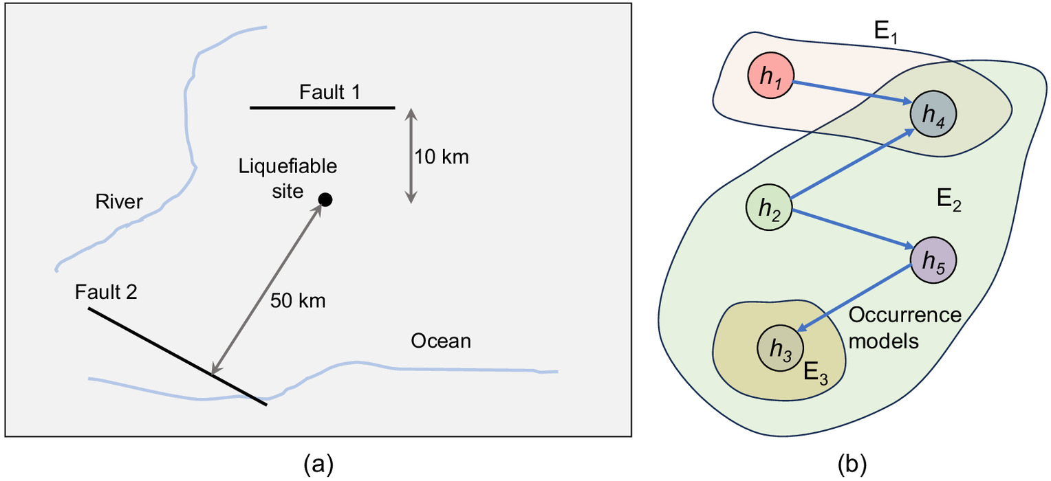
For directed hypergraphs, in each edge, the vertex can further be divided into source (so-called in hypergraph theory and not related to hazard sources as used in this paper) vertex set and target vertex set. For our purpose, the source vertex set represents the primary hazards in each edge, and the target vertex set represents all secondary hazards linked to each primary hazard for each edge. Eqs. (1) and (2) show the source () and target () matrices for Fig. 2(b). The number of edges () in Eqs. (1) and (2) corresponds to the number of primary hazards. The number of rows () in the source () and target () matrices corresponds to the total number of hazard sources in the region. For computation ease, the primary hazards are indexed before the secondary hazards, such that an identity matrix for the primary hazards can be derived from [see Eq. (1)]—i.e., , if or zero otherwise. Also, if the secondary hazard has a relationship/dependence with the primary hazard (in hypergraph ) or zero otherwise. In cases where a primary hazard triggers or alters the occurrence of a secondary hazard from the same source (e.g., mainshock-aftershock sequence from the same fault), the hazard is represented in both and —i.e., . We can also represent the primary hazards as a source unit column vector , with size ()where = earthquake from Fault 1; = earthquake from Fault 2; = flooding from river; = liquefaction from liquefiable site; and = tsunami from ocean.
(1)
(2)
The incidence matrix with size () for a directed hypergraph is given as follows:where and = target and source vertices for edge , respectively.
(3)
The directed hypergraph in Fig. 2(b) can be represented as shown in Eq. (4). In cases where a primary hazard triggers or alters the occurrence of a secondary hazard from the same source, the corresponding element in the incidence matrix is equal to unity—i.e.,
(4)
The hypergraph shown in Fig. 2(b) is static (i.e., with no temporal attributes). Hence, the incidence matrix developed from the static hypergraph [see Eq. (4)] cannot characterize the stochastic nature of multihazard interactions over a given time range. Such complex interactions and their stochastic nature cannot be represented with a static hypergraph but a temporal hypergraph. A temporal hypergraph is an assemble of hypergraphs with temporal attributes (e.g., time of hazard occurrence) associated with the vertices or edges—i.e., the temporal hypergraph is an assembly of static hypergraphs over a period [] (where ). The temporal attributes of the hypergraph can be defined using occurrence models and probabilistic simulation of events—described later in this section.
Defining Occurrence and Severity Models for Hazard Interaction Simulation
Reliable estimation of the frequency, timing, severity, and duration (especially for slow-onset events) of hazards is important for multihazard scenario simulation. The term severity is used in this study to refer to both event characteristics and local intensity measures. In fact, some aspects of hazard interactions may be governed by the event characteristics (i.e., the rate of aftershocks is governed by the magnitude of the mainshock). In contrast, others may be governed by the intensity measures (i.e., the triggering of a landslide following the occurrence of an earthquake is governed by the ground motion intensity at the slope location).
A set of occurrence and severity (including severity-time models for slow-onset hazards) models to capture the occurrence and interactions of hazards in the hypergraph edges must be defined for multihazard scenario simulation. The choice of occurrence and severity models depends on factors such as the nature of the hazard, available data, modeling objectives, and computational resources. Providing a detailed overview of all occurrence and severity models is outside the scope of this study. However, we highlight a few occurrence and severity models to support the discussions in this paper.
Hazard occurrence can be represented using homogeneous (HPP) and nonhomogeneous (NHPP) Poisson processes [e.g., hurricane—(Elsner et al. 2004); earthquakes—(Kagan and Jackson 1991); wind—(Gusclla 1991); floods—(Shane and Lynn 1964)], Weibull processes [e.g., flood—(Heo et al. 2001); earthquakes—(Hagiwara 1974); wind—(Xiao et al. 2006)], Brownian passage time (BPT) models [e.g., earthquakes—(Matthews et al. 2002)], among many others. Occurrence models typically combine various models that are based on input features such as environmental variables, land use, and other socioeconomic parameters. For example, flood occurrence can be simulated by combining rainfall-run-off models and hydraulic models (Rasouli et al. 2012; Schumann et al. 2013; Teng et al. 2017; Gori et al. 2019; Moftakhari et al. 2019). Studies (e.g., Gabriel et al. 2017; Oliveira et al. 2012) have also developed wildfire occurrence models that link meteorological factors (e.g., temperature, precipitation, wind speed) and land use. Also, drought occurrence can be simulated using the standardized precipitation index (SPI) (McKee et al. 1993) and/or the standardized soil moisture index SSMI (Hao and AghaKouchak 2013).
For triggering and altering interactions, the occurrence probability (or the rate curve relating the event characteristics to their corresponding exceedance rates) of a secondary hazard (say ) over a time interval (] is typically conditioned on the severity () and the occurrence rate () of the primary hazard (say ). For example, for an HPP, assuming that is triggered if reaches a certain intensity threshold , the probability of occurrence of is given by Eq. (5). For example, as demonstrated in the case study presented subsequently in this paper, the simulation of the occurrence of earthquake-induced liquefaction could entail combining probabilistic liquefaction index models (e.g., Idriss and Boulanger 2010) with probabilistic local seismic intensity measure models [e.g., Boore et al. (2014) model] and earthquake occurrence models (e.g., Cornell and Vanmarcke 1969)
(5)
The alteration interaction (i.e., the increased or decreased occurrence rate or severity of a secondary hazard) can generally be expressed as a function of the occurrence rate , severity of the primary hazard , the conditional occurrence model of the secondary hazard, —e.g., the altered occurrence rate of a secondary hazard can be expressed as . Alteration interactions can be captured using a single or a combination of models. Several studies (e.g., Liu et al. 2010; Peters and Iverson 2017; Taufik et al. 2017) have developed models to simulate wildfire occurrence amplification in drought-affected areas. Also, climate change models (e.g., Lee et al. 2021) can be linked to occurrence models for hydrometeorological hazards to capture altering relationships between climate change and the meteorological factors present in these occurrence models. There may be instances where the relationship between two hazards is not straightforward (e.g., studies have considered mainshock-aftershock sequences as either triggered or altered relationships). In such situations, risk analysts can choose the occurrence models that best align with the relationship they assume.
For rapid-onset processes, only single-point interarrival times, simulated from the defined stochastic process, are needed for scenario modeling. For example, for an NHPP, a thinning algorithm (Lewis and Shedler 1979) can be used to generate the interarrival times and the event duration is assumed to be zero (i.e., negligible with respect to the typical time range—e.g., 50 or 100 years) for multihazard scenario simulation. Similarly, severity models for rapid-onset processes can be used to generate a single point severity metric [e.g., tsunami inundation depth—see Abe (1995) and Kulikov et al. (2005)]. For slow-onset processes, the process duration and severity fluctuation during the process need to be characterized. For example, studies (e.g., Kirono et al. 2020; Sharma and Panu 2012) provide probabilistic models for predicting the duration of drought events as a function of SPI. The severity models for slow-onset typically generate a severity-time series—e.g., time series of drought index (e.g., Kirono et al. 2020).
Probabilistic Simulation of Multihazard Scenarios
Once the occurrence and severity models are defined for each hazard type of interest, a probabilistic simulation of multihazard events can be carried out. The flowchart for the multihazard scenario simulation within a desired time interval [] is presented in Figs. 3 and 4. To start the analysis, we initialize the initial time and set , and . Subsequently, the arrival times of all primary hazards in the source column vector () are simulated using the defined occurrence models. We then set the occurrence times as the sum of and . Subsequently, we set the current time to be the minimum of the simulated occurrence times of the primary hazards [i.e., ]. As shown in Fig. 3, if exceeds the defined , we assume that no event will happen within the defined time interval [] and end the simulation. Otherwise, we proceed with simulating the occurrence of the current primary hazard at the current time. The hypergraph incidence matrix at time (i.e., ) is updated to reflect the occurrence of (i.e., the hypergraph at the time of occurrence of the primary hazard is updated accordingly— equals 1 for simulated primary hazard). We then use the defined severity models to simulate the severity of at , . Fig. 5 illustrates a hypothetical multihazard analysis for the region in Fig. 2 to generate an array of incidence and severity matrices across the time interval.
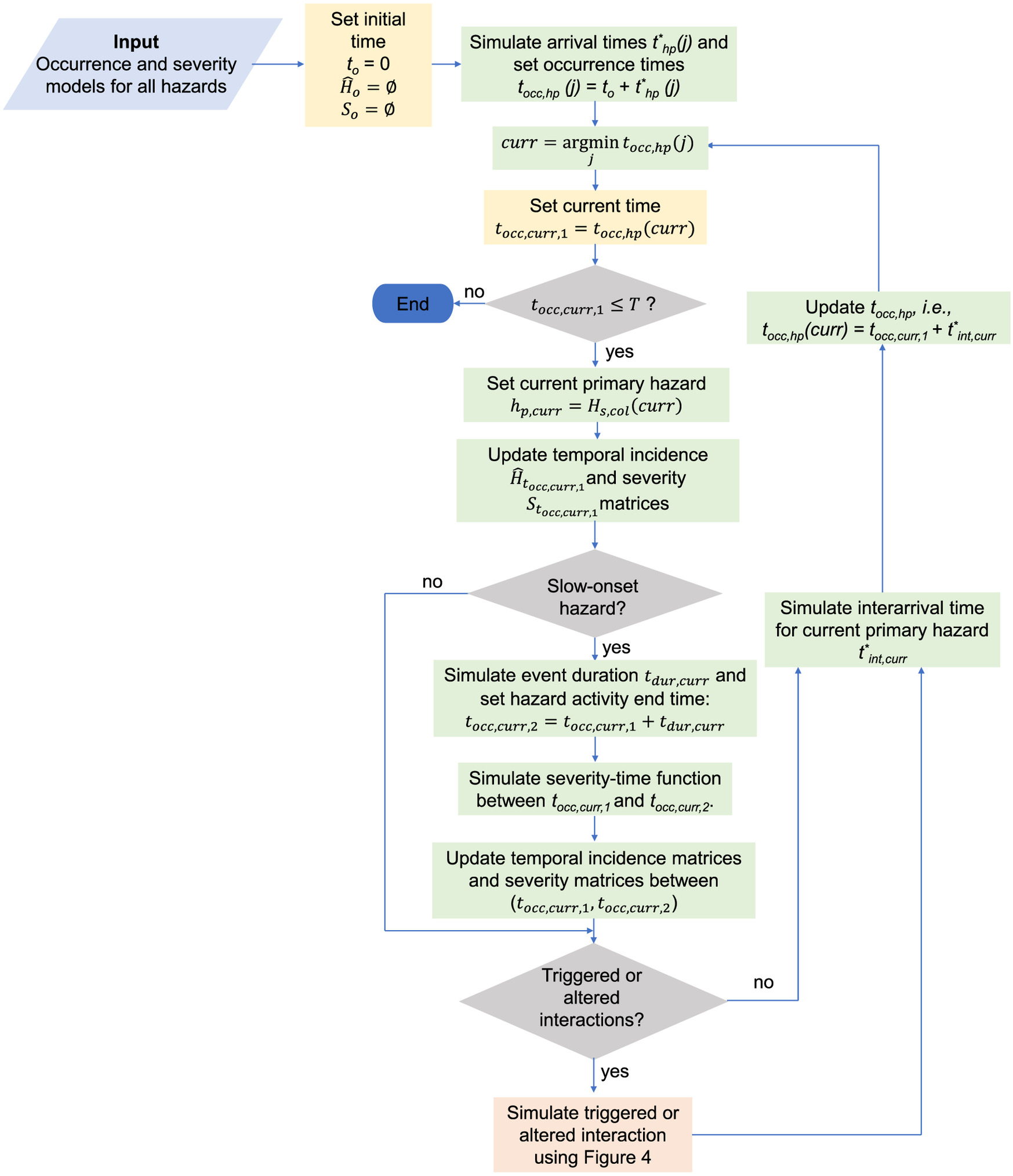
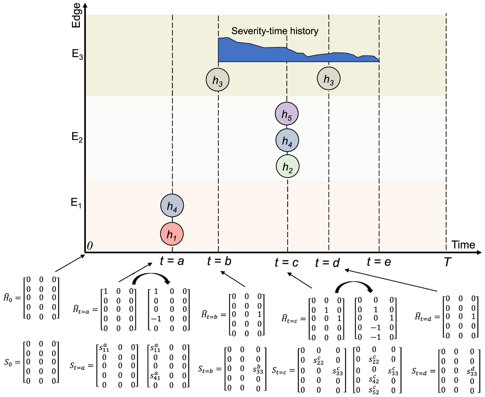
The next step is to simulate the temporal features of —i.e., the event duration and severity-time series. For rapid-onset processes (e.g., earthquakes and tsunami), event duration can be assumed to be zero, and the event is represented as a point in time—i.e., event end time and only appear in one hypergraph incidence matrix and severity matrix. For example, Fig. 5 depicts , , , and as rapid-onset hazards; hence, each of their occurrences is represented in a single incidence matrix and a single severity matrix.
For slow-onset processes, . The associated severity fluctuation between times and for slow-onset processes can be simulated using relevant duration forecasting approaches. Slow-onset processes can appear in more than one hypergraph and severity incidence matrices. The number of defined hypergraph and severity incidence matrices depends on a predefined timestep. The timestep should be set such that the peaks and troughs of the severity-time series are properly captured. This is crucial for properly defining the corresponding severity matrices within the time range (i.e., and ). Fig. 5 depicts as a slow-onset process occurring between time and with a simulated severity-time history (e.g., maximum inundation depth versus time). The corresponding severity (—where, = hazard, = edge, = current time) at each timestep can be derived from the severity-time series.
The next step is to simulate the impact of the occurrence of the current primary hazard on other hazards. As shown in Fig. 3, if the current primary hazard has no interactions with other hazards, we proceed to simulate a new interarrival time and next occurrence time of the primary hazard , and then update . Subsequently, the entire hazard occurrence simulation process is repeated with the updated for the primary hazard with the updated .
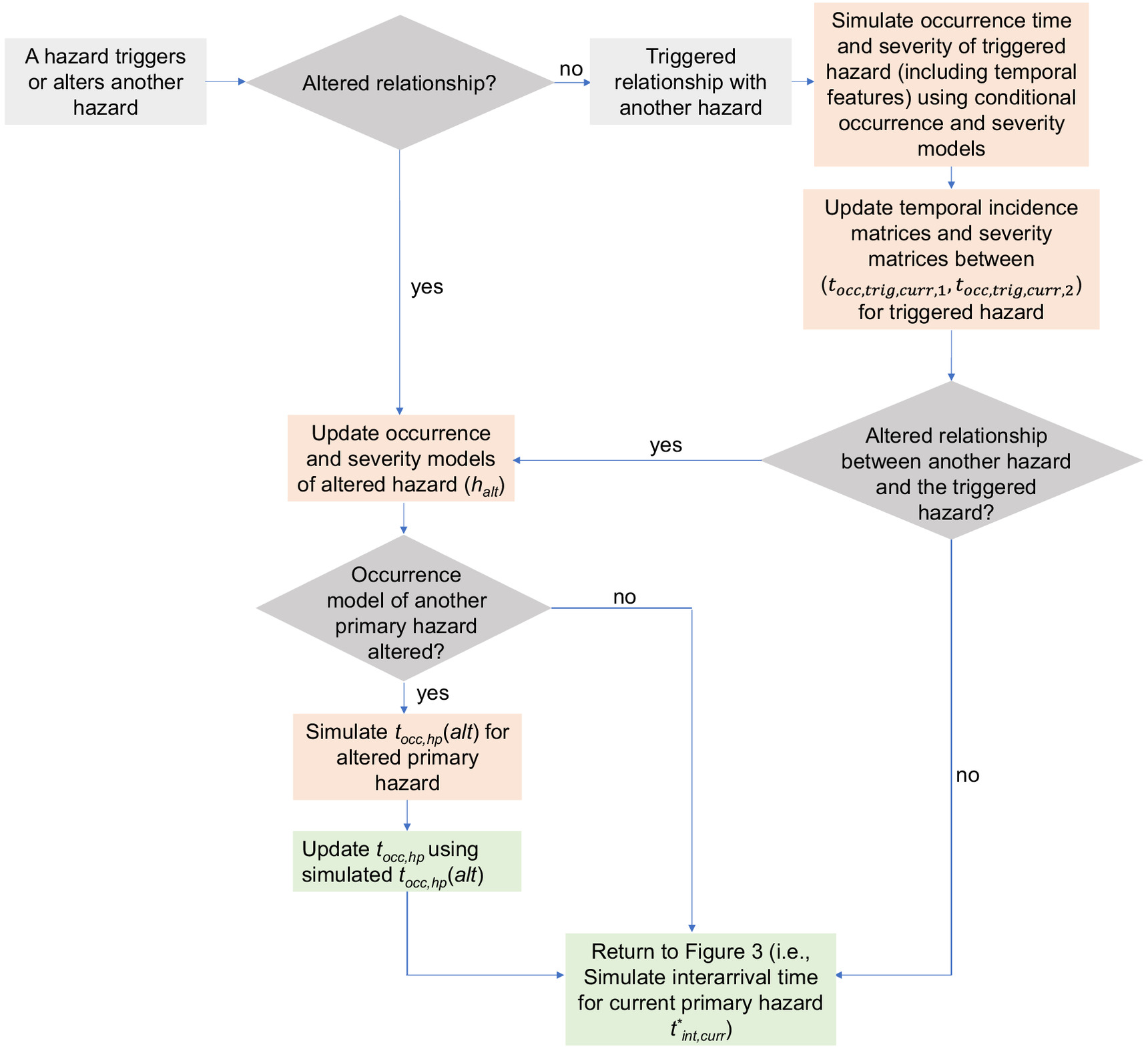
As shown in Fig. 3, if the current primary hazard has an altered or triggered interaction with other hazards, we simulate each interaction using the flowchart presented in Fig. 4. If an altered interaction exists between the simulated primary hazard and other hazards, for each altered hazard, we update their corresponding occurrence and severity models accordingly (i.e., using the predefined occurrence and severity models). If the altered hazard is contained in , we use the updated occurrence model to simulate a new arrival time and new occurrence time for this altered primary hazard and update .
In the case of triggered interactions, we simulate the occurrence time and severity of the triggered hazards (including temporal features) using corresponding conditional occurrence and severity models. Similar to the process for the primary hazard, the start time and end time (if slow-onset process) of the triggered hazard is simulated. Furthermore, we update the hypergraph incidence matrices and the severity matrices–i.e., for equals for the simulated secondary hazard (as a result of the occurrence of the primary hazard) at time (see Fig. 5). As shown in Fig. 4, the framework also captures scenarios where a triggered hazard could alter the severity and/or occurrence models of other hazards.
As shown in Fig. 3, the simulation continues until a is not achieved. The simulation of multihazard events will generate a number of hypergraph incidence matrices similar to those in Fig. 5. Once the simulation is complete [i.e., ], all the hypergraphs can be aggregated together to develop the multihazard scenario shown in Fig. 5.
Event Coincidence Analysis: Capturing Independent Concurrent Occurrence Using Sliding Window for Temporal Hypergraphs
The identification of concurrent independent hazards is important for multihazard risk management purposes. For example, about 70 countries reported flooding events during the COVID-19 pandemic (Simonovic et al. 2021). Apart from overlapping independent occurrences, there is also a coincidence window for the joint impact of independent hazards occurring in close proximity. For example, a catastrophic flood occurred roughly a month after the 2023 Turkish-Syria earthquake sequence, further affecting the earthquake victims (Kirby 2023).
The joint occurrence of independent hazards can be captured using event coincidence analysis (ECA) (e.g., Donges et al. 2016). This study adopts the sliding window procedure for temporal hypergraphs, widely used for signal processing (Myers et al. 2023), for event coincidence analysis (i.e., to capture the concurrent occurrence of independent hazards). In the sliding window procedure, a window of specified width (hereafter referred to as the coincidence interval) , slides along the time domain of a temporal hypergraph and segments the time series into windows that can be used for consequence/impact analysis. For example, given a hypergraph time domain of , a coincidence interval of , and a shift (where ), it is possible to create a set of windows () with time intervals
(6)
As Donges et al. (2016) described, the ECA only considers the coincidence interval. The sliding window procedure adds more flexibility to defining coincidence windows using the shift parameter.
Each sliding window can be used to create a hypergraph snapshot by including any edge with a nonempty intersection between the sliding window interval and the edge’s interval set. The presence of two edges in a sliding window interval signifies independent concurrent occurrences. This is written aswhere = edge (i.e., hazard relationship) in the set of edges defined in the static hypergraph; and = interval collection for edge .
(7)
The collection of the hypergraph snapshots , can be cast as a discrete dynamical process () to gain insight into the multihazard dynamics of the region in a considered timeframe (i.e., providing a temporal attribute). Each hypergraph snapshot can be mathematically expressed using a window incidence matrix (referred to in this paper as window incidence matrix to differentiate it from the static incidence matrix that is defined for a point in time) with elements , where the column elements represent the edges and the rows represent the hazard sources . The window incidence matrix depicts the occurrence of a primary or secondary hazard, linked to a particular single-hazard or multihazard relationship at a given window. Similar to a static incidence matrix, a window incidence matrix element is 0, if , 1 if the hazard is primary, and if secondary.
Stakeholders may choose to select a desired coincidence window (e.g., or 2 months) to characterize the joint occurrence of earthquake and flood hazards because it allows them to implement adequate flood-proof postearthquake recovery management strategies within the first two months of a big earthquake. The illustrative example presented in this paper demonstrates the significance of selected and on the temporal incidence matrix and capturing independent concurrent occurrences.
Illustrative Example
The proposed methodology is illustrated on the simple testbed region shown in Fig. 2. Future studies will explore applying the methodology to realistic testbeds. In this illustrative example, it is assumed that decision-makers are interested in multihazard events to assist with disaster management policies in the community. Following the steps outlined in Fig. 1, the hazard sources and interactions in the community have been characterized using the hypergraph in Fig. 2(b). The illustrative example will focus on defining the occurrence models, simulation of multihazard events, and sliding window analysis.
Occurrence Models
We consider a simple case where Fault 1 produces earthquakes with (moment) magnitudes at a constant rate of 0.01 per year. Fault 2 produces earthquakes with magnitudes at a rate of 0.025 per year. In other words, for the mainshocks, we assume for simplicity (and for illustrative purposes only) an HPP for interarrival time simulation and the doubly bounded exponential function (Cornell and Vanmarcke 1969) for earthquake magnitude simulation. Both faults are assumed to be strike-slip faults. Local seismic IMs—in terms of peak ground and spectral accelerations—are simulated according to the ground motion model of Boore et al. (2014) for illustrative purposes (any other relevant ground motion model for the region of interest could be used). The soil conditions are described later in this section. Note that, even if not very common, a strike-slip fault can generate a tsunami, as in the considered example (e.g., Ho et al. 2021). For instance, if a strike-slip fault is located near a shallow bay or a narrow inlet, the horizontal motion of the fault can push water into or out of the bay, creating a surge or a drawdown of the water level. This can amplify the wave height and cause flooding or erosion along the coast. An example is the 2018 Palu tsunami in Indonesia, triggered by a magnitude 7.5 strike-slip earthquake along the Palu-Koro fault (Ho et al. 2021). The earthquake caused a southward displacement of the seafloor along the Makassar Strait, which generated a long-wave tsunami that propagated into the Palu Bay and reached up to six meters high.
The aftershock sequence for the two faults is modeled using the BASS model (Turcotte et al. 2007). Other aftershock sequence modeling/simulation approaches [e.g., ETAS (Ogata 1998) and equivalent Poisson through Omori law (Shcherbakov et al. 2005)] can also be adopted here. Specifically, the BASS model is used to simulate the number, magnitude, occurrence time, and location of aftershocks, as shown in Eqs. (8)–(11), respectivelywhere = number of offspring earthquakes with magnitude greater than the specified minimum magnitude ; = difference between the magnitude of the parent earthquake and the largest aftershock [see modified Båth’s law (Shcherbakov et al. 2005)], = parameter of the Gutenberg-Richter (GR) distribution; and = temporal Omori parameters (Shcherbakov et al. 2004); and = spatial Omori parameters (Helmstetter and Sornette 2003); and , , and = cumulative distribution functions for the magnitude, time, and distance of the offspring earthquake, respectively. The GR-Båth, temporal Omori, and spatial Omori parameters used in carrying out BASS simulation in this study (see Table 1) are based on Turcotte et al. (2007). For the purpose of this study, similar parameters are assumed for both faults.
(8)
(9)
(10)
(11)
| 1.0 | 1.25 | 0.1 days | 1.25 | 3.5 m | 1.35 | 5 |
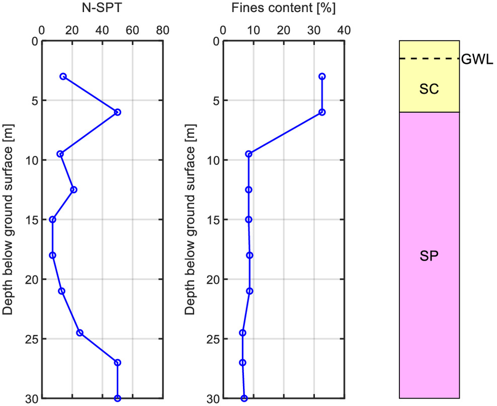
The considered liquefaction occurrence model combines the peak ground acceleration (PGA) at the site with the geotechnical parameters of the liquefiable site to simulate earthquake-induced liquefaction occurrence. The probabilistic distribution of PGA at the liquefiable site is estimated using the Boore et al. (2014) model, assuming equals . As shown in Fig. 2, the distance between the liquefiable site and Faults 1 and 2 are 10 km and 50 km, respectively. The assumed borehole data for the liquefiable site is shown in Fig. 6. The depth of the groundwater level at the site is taken as 1.5 m. Two soil types—clayey sand (SC) and poorly graded sand (SP) are assumed for the site. The soil density parameters are and for dry and wet soil, respectively. For this study, we assume the liquefaction occurrence time ≈ occurrence time of triggering earthquake.
The probability of liquefaction () can be estimated as (Idriss and Boulanger 2010)where = standard normal cumulative distribution function; and = factor of safety against the liquefaction for each layer. Other models (e.g., Cetin et al. 2004; Juang et al. 2012; Li et al. 2006) can be adopted as well.
(12)
The factor of safety is estimated aswhere = cyclic resistance ratio calibrated for a M7.5 earthquake and is estimated using Eq. (14) (Idriss and Boulanger 2006); CSR = cyclic shear ratio and is estimated using Eq. (15) (Seed and Idriss 1971). The magnitude scaling factor (MSF) accounts for shaking duration impacts, and is the overburden correction factor (Idriss and Boulanger 2006)where = equivalent clean-sand SPT blow estimated according to Idriss and Boulanger (2006)where = total vertical stress; = effective vertical stress at depth ; = peak horizontal ground acceleration (i.e., PGA) at the ground surface; = gravitational acceleration; and = stress reduction factor that accounts for the flexibility of the soil column, estimated according to Idriss and Boulanger (2006).
(13)
(14)
(15)
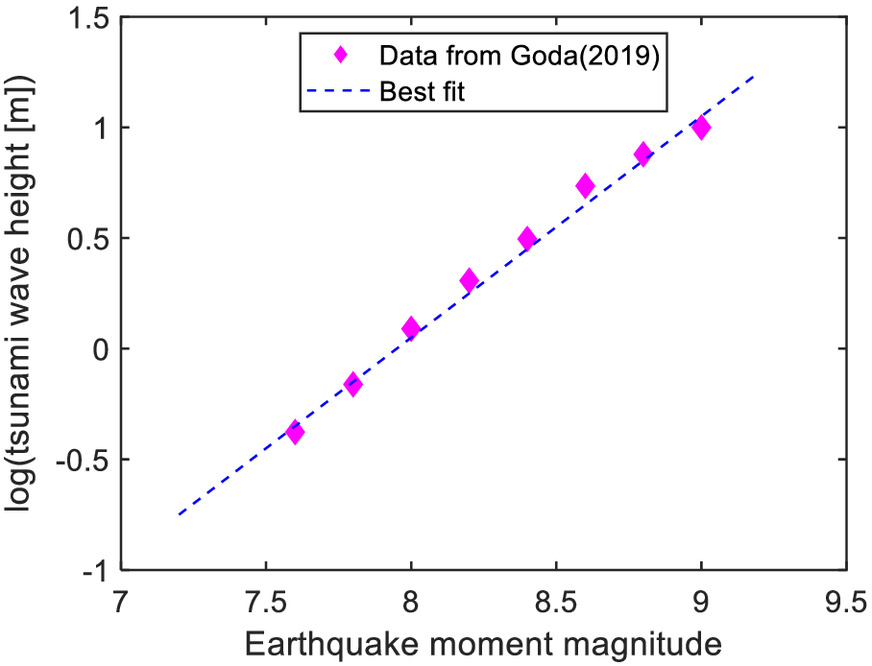
A detailed probabilistic tsunami hazard analysis (PTHA) (e.g., Geist and Parsons 2006; Goda 2019; Horspool et al. 2014), which relies on numerical tsunami propagation methods, is required to simulate the tsunami runup height. Such analyses typically account for the topographic and hydrodynamic characteristics of the site and tsunami waves. For the intended illustration purpose of this section, rather than carry out a PTHA, we use the PTHA output from Goda (2019) [i.e., cumulative distribution functions (CDF) of tsunami wave height for different earthquake magnitudes] based on heterogeneous slip models for our tsunami severity model. Given that Goda (2019) provides CDFs for only eight magnitudes, we fit an exponential function to the median estimates of the CDFs for interpolation purposes [Fig. 7 and Eq. (16)]. As shown in Fig. 7, the tsunami wave height can be expressed as a function of earthquake magnitude only. We note that other studies (e.g., Abe 1995; Kulikov et al. 2005) have developed similar expressions using actual data from tsunamigenic earthquakes. A lognormal distribution with a standard deviation of 0.33 is associated with Eq. (16). Similar to the liquefaction hazard, we make a deterministic assumption that the arrival time of the tsunami wave ≈ occurrence time of the triggering earthquake (e.g., Carvajal et al. 2019)
(16)
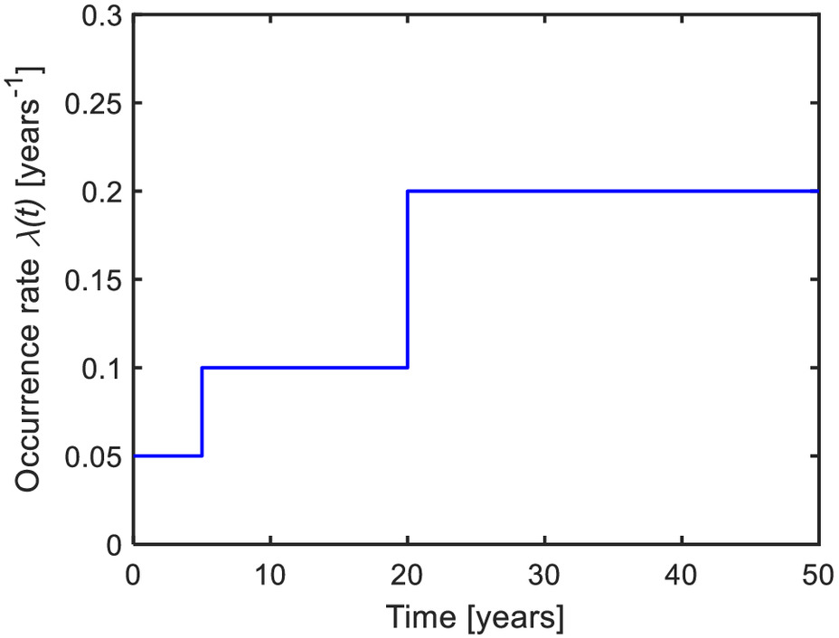
In this example, climate change is assumed to influence the flood-inducing processes (i.e., snowmelt or extreme precipitation), resulting in a time-varying flood occurrence rate shown in Fig. 8. The hypothetical time-varying flood occurrence rate in Fig. 8 is informed by existing studies (e.g., Berghuijs et al. 2017; Mudelsee et al. 2004). In this paper, we make a simple assumption that the yearly maximum flood depth associated with climate-induced flood () follows a lognormal distribution with a time-varying relationship shown in Eq. (17) and a standard deviation of 0.4 m. Eq. (17) follows conclusions from studies (e.g., Kuok et al. 2022) that flood depth can increase by 1 m every 30 years. Similarly, other flood severity parameters (e.g., flood discharge) are not simulated for simplicity. Sophisticated hydrological and hydrodynamic models [see Schumann et al. (2013) and Yamazaki et al. (2013)] that account for topography and hydrodynamics can be used to simulate the severity and local intensity of flood hazards. However, such models may be computationally expensive. Simplified occurrence and severity models can be used, provided the trade-off between model simplicity, analysis time, and accuracy of results is justified.
Furthermore, we assume that any tsunami hazard with tsunami runup height triggers river overflow in the area. The maximum flood depth associated with the tsunami-induced flood () is hypothetically assumed to be dependent on the tsunami runup height using Eq. (18). We note that Eq. (18) is not based on actual data but only used here for illustrative purposes. Eq. (18) is assumed to provide a median estimate with a lognormal standard deviation of 0.5 m. It is also assumed that the arrival time of the tsunami-induced flood ≈ arrival time of the tsunami wave
(17)
(18)
Probabilistic Simulation
Edges and
For each fault, we estimate the occurrence time of the earthquake (based on the HPP assumption). As depicted in Fig. 3, the mainshock event is only considered if the simulated mainshock time . If , the corresponding mainshock magnitude is simulated through the doubly bounded exponential function (Cornell and Vanmarcke 1969). For each simulated mainshock magnitude, we simulate the number, magnitude, occurrence time, and location of aftershocks using Eqs. (8)–(11), respectively. As an example, if a mainshock has a magnitude of 7.1, using the parameters in Table 1 in Eq. (8), the number of aftershocks is estimated as seven. For one of the seven aftershocks, assuming we simulate , , and , an aftershock with magnitude 5.17 at time 0.0261 days (0.63 h) from the mainshock arrival time and radial distance of 20.3 km from the mainshock is estimated. Once the magnitude and time of each aftershock are estimated, the aftershocks are treated as parent earthquakes, and higher orders of aftershock sequences are simulated until no more aftershocks are generated within the time .
For the earthquake-tsunami sequence, for a mainshock magnitude of 7.1, a median tsunami runup height of 1.82 m is estimated. The median runup height and the lognormal standard deviation are then used to simulate the runup height. For example, if the simulated random number equals 0.537, the simulated runup height is estimated as 1.9 m. Given that the runup height is , following the assumption of the illustrative study, a flood hazard is triggered, and the maximum flood depth is also simulated from the median estimate [Eq. (18)] and the lognormal standard deviation of 0.4.
Edges
Given that the flood occurrence model is time-varying, the thinning algorithm (Lewis and Shedler 1979) for NHPP is adopted here. We simulate the corresponding maximum flood depth for each simulated occurrence time using a median estimate derived from Eq. (17) and the lognormal standard deviation of 0.5, as discussed previously.
Simulation Output
The probabilistic scenario analysis can be performed to identify various interactions in time and space, producing a stochastic hazard sequence (or event set). Fig. 9 shows an example of a simulated event set for occurrence times and severities of the primary and secondary hazards in the three edges. In this particular event set, Fault 2 (primary hazard of ) generates a M7.2 earthquake (in year 12) that triggers a tsunami with runup height of 1.2 m. The tsunami floods the river with a maximum flood depth of 0.25 m. The mainshock produces nine aftershocks with magnitudes ranging from M5.0 to M5.6, and occurring between 0.1 days and 85 days after the mainshock.
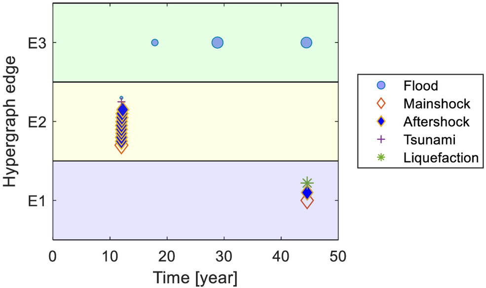
Three primary flood events are simulated in edge . The first flood event has a maximum flood depth of 1.7 m and occurs in year 17.9. The second and third events have a maximum flood depth of 4.9 m and 4.6 m, respectively, and occur in years 28.8 and 44.4, respectively.
Finally, Fault 1 generates a M6 earthquake in year 44.6, triggering liquefaction on the liquefiable site and an aftershock of M5.1 about 0.4 days after the mainshock.
Sliding Window Analysis
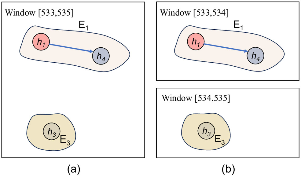
The sliding window procedure can identify the joint occurrence of two independent events from different edges in a simulated event set. As mentioned earlier, the output of the sliding window procedure is temporal incidence matrices that highlight the joint occurrence of events over the specified sliding window. It is evident from Fig. 9 that the third primary flood event (month 533.12) occurs around a similar period as the seismic activity in Fault 1 (month 534.6). However, this could be missed in a numerical analysis without a sliding window analysis or if an unfavorably small window width is specified.
Let us assume decision-makers have defined two months as the upper bound limit to define the joint occurrence of two hazards for planning purposes. Fig. 10 presents the hypergraph snapshots generated from the sliding procedure with two combinations of and around the occurrence time of the third primary flood and seismic event in Fault 1. As shown in Fig. 10(a), by adopting months and [i.e., (in months) = ] we capture the joint occurrence of the third primary flood event and the seismic activity of Fault 1 in {i.e., window [533,535]} [see Eq. (19)]. Alternatively, if we adopt and [i.e., (in months) = ], the joint occurrence of both primary hazards is missed [see Eq. (20) and Fig. 10(b)]
(19)
(20)
Information derived from the sliding window analysis (i.e., hypergraph snapshots and window incidence matrix) can be used to design or assess multihazard management strategies. Furthermore, as mentioned earlier, the sliding analysis can help capture independent events occurring in quick succession. The window incidence matrices can be used, for instance, to define scenarios for post-disaster recovery analysis (e.g., Opabola and Galasso 2024) of civil infrastructure susceptible to multiple hazards.
Conclusions
This study seeks to contribute to advancing multihazard performance-based engineering by developing a probabilistic framework for simulating multihazard scenarios for the design and risk assessment of civil infrastructure. The proposed entails (1) identifying all potential hazard sources in the geographical region of interest; (2) defining their potential hazard interrelationships (i.e., hazard interactions); (3) defining relevant occurrence models to simulate the identified for each hazard considering the interactions; (4) probabilistic simulation of multihazard event sets (i.e., interactions) over a defined space-time domain; and (5) event coincidence analysis to capture independent concurrent hazards.
The hazard source identification entails, for instance, collecting information on the location and history of seismic faults, volcanoes, flood sources (e.g., rainfall and other meteorological data, river/stream locations, and streamflow and water level data), and liquefaction- and landslide-prone areas. The hazard interrelationship definition entails defining the connections between hazards (i.e., primary and secondary hazards) and the mutual dependencies or influences between hazards. This study adopts the temporal hypergraph theory, widely used in network engineering, to characterize such hazard interactions. Once the hazard interrelationships are defined, relevant occurrence and severity models are defined for each primary and secondary hazard. Subsequently, simulation-based approaches are used to generate the arrival times and features (e.g., severity and/or local intensities) of all considered primary and secondary hazards over a defined space-time interval. Finally, the joint occurrence of independent concurrent hazards is captured using an event coincidence analysis (ECA). This study uses the sliding window analysis for the ECA process. In the sliding window procedure, coincidence interval and shift parameters are specified to develop a coincidence window for which any multiple independent hazards with arrival times in this window are assumed to be occurring concurrently.
The framework’s applicability is demonstrated using an illustrative example of a hypothetical region susceptible to earthquake-induced ground shaking, liquefaction, tsunami, and riverine flooding. In the illustrative example, reasonable assumptions for hazard parameters (i.e., occurrence and severity models) are used to simulate an event set for the community over a time range of 50 years.
The proposed modeling framework can be combined with vulnerability/impact assessment methodologies to quantify the multihazard risk of communities. Furthermore, generated event sets can help decision-makers design and test preparedness, mitigation, and recovery management policies.
Data Availability Statement
Some or all data, models, or code that support the findings of this study are available from the corresponding author upon reasonable request.
Acknowledgments
The author would like to acknowledge the fruitful discussions with Professor Carmine Galasso during the initial phase of the study. Also, the significant input of the two anonymous reviewers are acknowledged.
References
Abe, K. 1995. “Estimate of tsunami runup heights from earthquake magnitudes.” In Tsunami: Progress in prediction, disaster prevention and warning, 21–35. New York: Springer.
Amini, A., N. Firouzkouhi, A. Gholami, A. R. Gupta, C. Cheng, and B. Davvaz. 2022. “Soft hypergraph for modeling global interactions via social media networks.” Expert Syst. Appl. 203 (Jan): 117466. https://doi.org/10.1016/j.eswa.2022.117466.
Berge, C. 1989. Hypergraphs: Combinatorics of finite sets. Amsterdam, Netherlands: Elsevier.
Berghuijs, W. R., E. E. Aalbers, J. R. Larsen, R. Trancoso, and R. A. Woods. 2017. “Recent changes in extreme floods across multiple continents.” Environ. Res. Lett. 12 (11): 114035. https://doi.org/10.1088/1748-9326/aa8847.
Boore, D. M., J. P. Stewart, E. Seyhan, and G. M. Atkinson. 2014. “NGA-West2 equations for predicting PGA, PGV, and 5% damped PSA for shallow crustal earthquakes.” Earthquake Spectra 30 (3): 1057–1085. https://doi.org/10.1193/070113EQS184M.
Bretto, A., and L. Gillibert. 2005. “Hypergraph-based image representation.” In Proc., Graph-Based Representations in Pattern Recognition: 5th IAPR Int. Workshop, GbRPR 2005, Poitiers, 1–11. New York: Springer.
Carvajal, M., C. Araya-Cornejo, I. Sepúlveda, D. Melnick, and J. S. Haase. 2019. “Nearly instantaneous tsunamis following the 7.5 2018 Palu Earthquake.” Geophys. Res. Lett. 46 (10): 5117–5126. https://doi.org/10.1029/2019GL082578.
Cetin, K. O., R. B. Seed, A. Der Kiureghian, K. Tokimatsu, L. F. Harder Jr., R. E. Kayen, and R. E. S. Moss. 2004. “Standard penetration test-based probabilistic and deterministic assessment of seismic soil liquefaction potential.” J. Geotech. Geoenviron. Eng. 130 (12): 1314–1340. https://doi.org/10.1061/(ASCE)1090-0241(2004)130:12(1314).
Cilia, M. G., W. D. Mooney, and C. Nugroho. 2021. “Field insights and analysis of the 2018 Mw 7.5 Palu, Indonesia Earthquake, tsunami and landslides.” Pure Appl. Geophys. 178 (12): 4891–4920. https://doi.org/10.1007/s00024-021-02852-6.
Cornell, C. A., and E. H. Vanmarcke. 1969. “The major influences on seismic risk.” In Vol. 1 of Proc., Fourth World Conf. on Earthquake Engineering, Santiago, Chile, session A–1, 69–83. New Delhi, India: Indian Institute of Technology Kanpur.
Decò, A., and D. M. Frangopol. 2011. “Risk assessment of highway bridges under multiple hazards.” J. Risk Res. 14 (9): 1057–1089. https://doi.org/10.1080/13669877.2011.571789.
Donges, J. F., C.-F. Schleussner, J. F. Siegmund, and R. V. Donner. 2016. “Event coincidence analysis for quantifying statistical interrelationships between event time series.” Eur. Phys. J. Spec. Top. 225 (3): 471–487. https://doi.org/10.1140/epjst/e2015-50233-y.
El Morjani, Z. E. A., S. Ebener, J. Boos, E. Abdel Ghaffar, and A. Musani. 2007. “Modelling the spatial distribution of five natural hazards in the context of the WHO/EMRO Atlas of Disaster Risk as a step towards the reduction of the health impact related to disasters.” Int. J. Health Geographics 6 (1): 8. https://doi.org/10.1186/1476-072X-6-8.
Elsner, J. B., X. Niu, and T. H. Jagger. 2004. “Detecting shifts in hurricane rates using a Markov Chain Monte Carlo approach.” J. Clim. 17 (13): 2652–2666. https://doi.org/10.1175/1520-0442(2004)017%3C2652:DSIHRU%3E2.0.CO;2.
Gabriel, E., T. Opitz, and F. Bonneu. 2017. “Detecting and modeling multi-scale space-time structures: The case of wildfire occurrences.” J. Soc. Fr. Statistique 158 (3): 86–105.
Geist, E. L., and T. Parsons. 2006. “Probabilistic analysis of tsunami hazards.” Nat. Hazards 37 (3): 277–314. https://doi.org/10.1007/s11069-005-4646-z.
Gill, J. C., and B. D. Malamud. 2014. “Reviewing and visualizing the interactions of natural hazards.” Rev. Geophys. 52 (4): 680–722. https://doi.org/10.1002/2013RG000445.
Gill, J. C., B. D. Malamud, E. M. Barillas, and A. Guerra Noriega. 2020. “Construction of regional multihazard interaction frameworks, with an application to Guatemala.” Nat. Hazards Earth Syst. Sci. 20 (1): 149–180. https://doi.org/10.5194/nhess-20-149-2020.
Goda, K. 2019. “Time-dependent probabilistic tsunami hazard analysis using stochastic rupture sources.” Stochastic Environ. Res. Risk Assess. 33 (2): 341–358. https://doi.org/10.1007/s00477-018-1634-x.
Gori, A., R. Blessing, A. Juan, S. Brody, and P. Bedient. 2019. “Characterizing urbanization impacts on floodplain through integrated land use, hydrologic, and hydraulic modeling.” J. Hydrol. 568 (Jan): 82–95. https://doi.org/10.1016/j.jhydrol.2018.10.053.
Green, R. A., M. Cubrinovski, B. Cox, C. Wood, L. Wotherspoon, B. Bradley, and B. Maurer. 2014. “Select liquefaction case histories from the 2010–2011 Canterbury earthquake sequence.” Earthquake Spectra 30 (1): 131–153. https://doi.org/10.1193/030713EQS066M.
Greiving, S., M. Fleischhauer, and J. Lückenkötter. 2006. “A methodology for an integrated risk assessment of spatially relevant hazards.” J. Environ. Plann. Manage. 49 (1): 1–19. https://doi.org/10.1080/09640560500372800.
Gusclla, V. 1991. “Estimation of extreme winds from short-term records.” J. Struct. Eng. 117 (2): 375–390. https://doi.org/10.1061/(ASCE)0733-9445(1991)117:2(375).
Hagiwara, Y. 1974. “Probability of earthquake occurrence as obtained from a Weibull distribution analysis of crustal strain.” Tectonophysics 23 (3): 313–318. https://doi.org/10.1016/0040-1951(74)90030-4.
Hao, Z., and A. AghaKouchak. 2013. “Multivariate standardized drought index: A parametric multi-index model.” Adv. Water Resour. 57 (Jan): 12–18. https://doi.org/10.1016/j.advwatres.2013.03.009.
Helmstetter, A., and D. Sornette. 2003. “Foreshocks explained by cascades of triggered seismicity.” J. Geophys. Res.: Solid Earth 107 (B10): 1–10. https://doi.org/10.1029/2001JB001580.
Heo, J.-H., J. D. Salas, and D. C. Boes. 2001. “Regional flood frequency analysis based on a Weibull model: Part 2. Simulations and applications.” J. Hydrol. 242 (3–4): 171–182. https://doi.org/10.1016/S0022-1694(00)00335-8.
Ho, T., K. Satake, S. Watada, M. Hsieh, R. Y. Chuang, Y. Aoki, I. E. Mulia, A. R. Gusman, and C. Lu. 2021. “Tsunami induced by the strike-slip fault of the 2018 Palu earthquake (), Sulawesi Island, Indonesia.” Earth Space Sci. 8 (6): e2020EA001400. https://doi.org/10.1029/2020EA001400.
Horspool, N., I. Pranantyo, J. Griffin, H. Latief, D. H. Natawidjaja, W. Kongko, A. Cipta, B. Bustaman, S. D. Anugrah, and H. K. Thio. 2014. “A probabilistic tsunami hazard assessment for Indonesia.” Nat. Hazards Earth Syst. Sci. 14 (11): 3105–3122. https://doi.org/10.5194/nhess-14-3105-2014.
Idriss, I. M., and R. W. Boulanger. 2006. “Semi-empirical procedures for evaluating liquefaction potential during earthquakes.” Soil Dyn. Earthquake Eng. 26 (2–4): 115–130. https://doi.org/10.1016/j.soildyn.2004.11.023.
Idriss, I. M., and R. W. Boulanger. 2010. SPT-based liquefaction triggering procedures. Davis, CA: Univ. of California Davis.
Johansson, J., H. Hassel, A. Cedergren, L. Svegrup, and B. Arvidsson. 2015. “Method for describing and analyzing cascading effects in past events: Initial conclusions and findings.” In Proc., European Safety and Reliability Conf. (ESREL2015). Amsterdam, Netherlands: CRC Press.
Jones, D. 1993. “Environmental hazards: The challenge of change: Environmental hazards in the 1990s: Problems, paradigms and prospects.” Geography 78 (2): 161–165.
Juang, C. H., J. Ching, Z. Luo, and C.-S. Ku. 2012. “New models for probability of liquefaction using standard penetration tests based on an updated database of case histories.” Eng. Geol. 133–134 (Apr): 85–93. https://doi.org/10.1016/j.enggeo.2012.02.015.
Kagan, Y. Y., and D. D. Jackson. 1991. “Long-term earthquake clustering.” Geophys. J. Int. 104 (1): 117–134. https://doi.org/10.1111/j.1365-246X.1991.tb02498.x.
Kameshwar, S., and J. E. Padgett. 2014. “Multihazard risk assessment of highway bridges subjected to earthquake and hurricane hazards.” Eng. Struct. 78 (Jun): 154–166. https://doi.org/10.1016/j.engstruct.2014.05.016.
Kappes, M. S., M. Keiler, and T. Glade. 2010. “From single- to multi-hazard risk analyses: A concept addressing emerging challenges.” In Proc., Mountains Risks: Bringing Science to Society (Int. Conf.), edited by J.-P. Malet, T. Glade, and N. Casagli, 351–356. Strassbourg, France: Centre for Education and Research in Geosciences Editions.
Kirby, P. 2023. “Turkish floods inundate two cities hit by quakes killing 14.” Accessed October 5, 2023. https://www.bbc.co.uk/news/world-europe-64968972.
Kirono, D. G. C., V. Round, C. Heady, F. H. S. Chiew, and S. Osbrough. 2020. “Drought projections for Australia: Updated results and analysis of model simulations.” Weather Clim. Extremes 30 (Jan): 100280. https://doi.org/10.1016/j.wace.2020.100280.
Konstantinova, E. V., and V. A. Skorobogatov. 2001. “Application of hypergraph theory in chemistry.” Discrete Math. 235 (1–3): 365–383. https://doi.org/10.1016/S0012-365X(00)00290-9.
Kulikov, E., A. B. Rabinovich, and R. E. Thomson. 2005. “Estimation of tsunami risk for the coasts of Peru and Northern Chile.” Nat. Hazards 35 (2): 185–209. https://doi.org/10.1007/s11069-004-4809-3.
Kuok, K. K., M. E. Mersal, P. C. Chiu, M. Y. Chin, M. R. Rahman, and M. K. B. Bakri. 2022. “Climate change impacts on sea level rise to flood depth and extent of Sarawak River.” Front. Water 4 (870936): 1–7. https://doi.org/10.3389/frwa.2022.870936.
Lee, J.-Y., J. Marotzke, G. Bala, L. Cao, S. Corti, J. P. Dunne, F. Engelbrecht, E. Fischer, J. C. Fyfe, and C. Jones. 2021. Future global climate: Scenario-based projections and near-term information. Geneva: Intergovernmental Panel on Climate Change.
Lewis, P. A. W., and G. S. Shedler. 1979. “Simulation of nonhomogeneous Poisson processes by thinning.” Nav. Res. Logist. Q. 26 (3): 403–413. https://doi.org/10.1002/nav.3800260304.
Li, D. K., C. H. Juang, and R. D. Andrus. 2006. “Liquefaction potential index: A critical assessment using probability concept.” J. GeoEng. 1 (1): 11–24.
Li, Y., Y. Dong, D. M. Frangopol, and D. Gautam. 2020. “Long-term resilience and loss assessment of highway bridges under multiple natural hazards.” Struct. Infrastruct. Eng. 16 (4): 626–641. https://doi.org/10.1080/15732479.2019.1699936.
Liu, B., Y. L. Siu, and G. Mitchell. 2016. “Hazard interaction analysis for multihazard risk assessment: A systematic classification based on hazard-forming environment.” Nat. Hazards Earth Syst. Sci. 16 (2): 629–642. https://doi.org/10.5194/nhess-16-629-2016.
Liu, Y., J. Stanturf, and S. Goodrick. 2010. “Wildfire potential evaluation during a drought event with a regional climate model and NDVI.” Ecol. Inf. 5 (5): 418–428. https://doi.org/10.1016/j.ecoinf.2010.04.001.
Matthews, M. V., W. L. Ellsworth, and P. A. Reasenberg. 2002. “A Brownian model for recurrent earthquakes.” Bull. Seismol. Soc. Am. 92 (6): 2233–2250. https://doi.org/10.1785/0120010267.
McKee, T. B., N. J. Doesken, and J. Kleist. 1993. “The relationship of drought frequency and duration to time scales.” In Proc., 8th Conf. on Applied Climatology, 179–183. Anaheim, CA: Integrated Drought Management Programme.
Ming, X., Q. Liang, R. Dawson, X. Xia, and J. Hou. 2022. “A quantitative multihazard risk assessment framework for compound flooding considering hazard inter-dependencies and interactions.” J. Hydrol. 607 (Apr): 127477. https://doi.org/10.1016/j.jhydrol.2022.127477.
Moftakhari, H., J. E. Schubert, A. AghaKouchak, R. A. Matthew, and B. F. Sanders. 2019. “Linking statistical and hydrodynamic modeling for compound flood hazard assessment in tidal channels and estuaries.” Adv. Water Resour. 128 (Jan): 28–38. https://doi.org/10.1016/j.advwatres.2019.04.009.
Mori, N., and T. Takahashi. 2012. “Nationwide post event survey and analysis of the 2011 Tohoku earthquake tsunami.” Coastal Eng. J. 54 (1): 1250001. https://doi.org/10.1142/S0578563412500015.
Mudelsee, M., M. Börngen, G. Tetzlaff, and U. Grünewald. 2004. “Extreme floods in central Europe over the past 500 years: Role of cyclone pathway ‘Zugstrasse Vb.’” J. Geophys. Res.: Atmos. 109 (D23): 1–21. https://doi.org/10.1029/2004JD005034.
Myers, A., C. Joslyn, B. Kay, E. Purvine, G. Roek, and M. Shapiro. 2023. “Topological analysis of temporal hypergraphs.” In International workshop on algorithms and models for the web-graph, 127–146. Cham, Switzerland: Springer.
Nguyen Sinh, H., F. T. Lombardo, C. W. Letchford, and D. V. Rosowsky. 2016. “Characterization of joint wind and ice hazard in Midwestern United States.” Nat. Hazard. Rev. 17 (3): 04016004. https://doi.org/10.1061/(ASCE)NH.1527-6996.0000221.
Ogata, Y. 1998. “Space-time point-process models for earthquake occurrences.” Ann. Inst. Stat. Math. 50 (2): 379–402. https://doi.org/10.1023/A:1003403601725.
Oliveira, S., F. Oehler, J. San-Miguel-Ayanz, A. Camia, and J. M. C. Pereira. 2012. “Modeling spatial patterns of fire occurrence in Mediterranean Europe using multiple regression and random forest.” For. Ecol. Manage. 275 (Jun): 117–129. https://doi.org/10.1016/j.foreco.2012.03.003.
Opabola, E. A., and C. Galasso. 2024. “A probabilistic framework for post-disaster recovery modeling of buildings and electric power networks in developing countries.” Reliab. Eng. Syst. Saf. 242 (Jan): 109679. https://doi.org/10.1016/j.ress.2023.109679.
Pescaroli, G., and D. Alexander. 2018. “Understanding compound, interconnected, interacting, and cascading risks: A holistic framework.” Risk Anal. 38 (11): 2245–2257. https://doi.org/10.1111/risa.13128.
Peters, M. P., and L. R. Iverson. 2017. “Incorporating fine-scale drought information into an eastern US wildfire hazard model.” Int. J. Wildland Fire 26 (5): 393. https://doi.org/10.1071/WF16130.
Petroliagkis, T. I., E. Voukouvalas, J. Disperati, and J. Bidlot. 2016. “Joint probabilities of storm surge, significant wave height and river discharge components of coastal flooding events—Utilizing statistical dependence methodologies & techniques.” Accessed April 13, 2016. https://data.europa.eu/doi/10.2788/677778.
Qie, Z., and L. Rong. 2022. “A scenario modelling method for regional cascading disaster risk to support emergency decision making.” Int. J. Disaster Risk Reduct. 77 (Jun): 103102. https://doi.org/10.1016/j.ijdrr.2022.103102.
Rasouli, K., W. W. Hsieh, and A. J. Cannon. 2012. “Daily streamflow forecasting by machine learning methods with weather and climate inputs.” J. Hydrol. 414–415 (Sep): 284–293. https://doi.org/10.1016/j.jhydrol.2011.10.039.
Rosowsky, D. V., and Y. Wang. 2012. “Joint wind-snow hazard characterization for reduced reference periods.” J. Perform. Constr. Facil. 28 (1): 121–127. https://doi.org/10.1061/(ASCE)CF.1943-5509.0000385.
Schmidt-Thomé, P., S. Greiving, H. Kallio, M. Fleischhauer, and J. Jarva. 2006. “Economic risk maps of floods and earthquakes for European regions.” Quat. Int. 150 (1): 103–112. https://doi.org/10.1016/j.quaint.2006.01.024.
Schumann, G. J.-P., J. C. Neal, N. Voisin, K. M. Andreadis, F. Pappenberger, N. Phanthuwongpakdee, A. C. Hall, and P. D. Bates. 2013. “A first large-scale flood inundation forecasting model.” Water Resour. Res. 49 (10): 6248–6257. https://doi.org/10.1002/wrcr.20521.
Seed, H. B., and I. M. Idriss. 1971. “Simplified procedure for evaluating soil liquefaction potential.” J. Soil Mech. Found. Div. 97 (9): 1249–1273. https://doi.org/10.1061/JSFEAQ.0001662.
Sevieri, G., C. Galasso, D. D’Ayala, R. De Jesus, A. Oreta, M. E. D. A. Grio, and R. Ibabao. 2020. “A multihazard risk prioritization framework for cultural heritage assets.” Nat. Hazards Earth Syst. Sci. 20 (5): 1391–1414. https://doi.org/10.5194/nhess-20-1391-2020.
Shane, R. M., and W. R. Lynn. 1964. “Mathematical model for flood risk evaluation.” J. Hydraul. Div. 90 (6): 1–20. https://doi.org/10.1061/JYCEAJ.0001127.
Sharma, T. C., and U. S. Panu. 2012. “Prediction of hydrological drought durations based on Markov chains: Case of the Canadian prairies.” Hydrol. Sci. J. 57 (4): 705–722. https://doi.org/10.1080/02626667.2012.672741.
Shcherbakov, R., D. L. Turcotte, and J. B. Rundle. 2004. “A generalized Omori’s law for earthquake aftershock decay.” Geophys. Res. Lett. 31 (11): 1–5. https://doi.org/10.1029/2004GL019808.
Shcherbakov, R., D. L. Turcotte, and J. B. Rundle. 2005. “Aftershock statistics.” Pure Appl. Geophys. 162 (6–7): 1051–1076. https://doi.org/10.1007/s00024-004-2661-8.
Simonovic, S. P., Z. W. Kundzewicz, and N. Wright. 2021. “Floods and the COVID-19 pandemic—A new double hazard problem.” WIREs Water 8 (2): e1509. https://doi.org/10.1002/wat2.1509.
Svensson, C., and D. A. Jones. 2002. “Dependence between extreme sea surge, river flow and precipitation in eastern Britain.” Int. J. Climatol. 22 (10): 1149–1168. https://doi.org/10.1002/joc.794.
Taufik, M., P. J. J. F. Torfs, R. Uijlenhoet, P. D. Jones, D. Murdiyarso, and H. A. J. Van Lanen. 2017. “Amplification of wildfire area burnt by hydrological drought in the humid tropics.” Nat. Clim. Change 7 (6): 428–431. https://doi.org/10.1038/nclimate3280.
Teng, J., A. J. Jakeman, J. Vaze, B. F. W. Croke, D. Dutta, and S. Kim. 2017. “Flood inundation modelling: A review of methods, recent advances and uncertainty analysis.” Environ. Modell. Software 90 (Dec): 201–216. https://doi.org/10.1016/j.envsoft.2017.01.006.
Tilloy, A., B. D. Malamud, H. Winter, and A. Joly-Laugel. 2019. “A review of quantification methodologies for multihazard interrelationships.” Earth Sci. Rev. 196 (Nov): 102881. https://doi.org/10.1016/j.earscirev.2019.102881.
Turcotte, D. L., J. R. Holliday, and J. B. Rundle. 2007. “BASS, an alternative to ETAS.” Geophys. Res. Lett. 34 (12): L12303. https://doi.org/10.1029/2007GL029696.
Xiao, Y. Q., Q. S. Li, Z. N. Li, Y. W. Chow, and G. Q. Li. 2006. “Probability distributions of extreme wind speed and its occurrence interval.” Eng. Struct. 28 (8): 1173–1181. https://doi.org/10.1016/j.engstruct.2006.01.001.
Yamazaki, D., G. A. M. de Almeida, and P. D. Bates. 2013. “Improving computational efficiency in global river models by implementing the local inertial flow equation and a vector-based river network map.” Water Resour. Res. 49 (11): 7221–7235. https://doi.org/10.1002/wrcr.20552.
Zaghi, A. E., J. E. Padgett, M. Bruneau, M. Barbato, Y. Li, J. Mitrani-Reiser, and A. McBride. 2016. “Establishing common nomenclature, characterizing the problem, and identifying future opportunities in multihazard design.” J. Struct. Eng. 142 (12): H2516001. https://doi.org/10.1061/(ASCE)ST.1943-541X.0001586.
Zellou, B., and H. Rahali. 2019. “Assessment of the joint impact of extreme rainfall and storm surge on the risk of flooding in a coastal area.” J. Hydrol. 569 (Sep): 647–665. https://doi.org/10.1016/j.jhydrol.2018.12.028.
Zheng, F., S. Westra, M. Leonard, and S. A. Sisson. 2014. “Modeling dependence between extreme rainfall and storm surge to estimate coastal flooding risk.” Water Resour. Res. 50 (3): 2050–2071. https://doi.org/10.1002/2013WR014616.
Zuccaro, G., D. De Gregorio, and M. F. Leone. 2018. “Theoretical model for cascading effects analyses.” Int. J. Disaster Risk Reduct. 30 (Sep): 199–215. https://doi.org/10.1016/j.ijdrr.2018.04.019.
Information & Authors
Information
Published In

Natural Hazards Review
Volume 25 • Issue 4 • November 2024
Copyright
This work is made available under the terms of the Creative Commons Attribution 4.0 International license, https://creativecommons.org/licenses/by/4.0/.
History
Received: Oct 8, 2023
Accepted: May 28, 2024
Published online: Aug 24, 2024
Published in print: Nov 1, 2024
Discussion open until: Jan 24, 2025
ASCE Technical Topics:
Authors
Metrics & Citations
Metrics
Citations
Download citation
If you have the appropriate software installed, you can download article citation data to the citation manager of your choice. Simply select your manager software from the list below and click Download.