Using Disaster Surveys to Model Business Interruption
Abstract
Business interruption after disasters is an important metric for community resilience planning because has both economic and social consequences. Each additional day that a business is nonoperational further compounds lost revenue, wages, and lack of access to goods and services needed for recovery. Therefore, the use of surveys has grown in the literature as a way to capture the diverse information needed for modeling business disaster outcomes. However, variable inclusion and measurement can vary widely across studies, and there is a lack of guidance on how to structure surveys most effectively to facilitate this effort. This study fills these gaps through an analysis of variable choice, variable measurement, and measurement timing using data from an interdisciplinary field study in Lumberton, North Carolina after 2016 Hurricane Matthew. We found that empirical business interruption models can be improved significantly by using a comprehensive set of utility and damage variables; integrating damage information based on damage states for building, contents, and machinery; and capturing recovery-time dynamics by using business downtime and utility outage durations, rather than binary measurements. The results suggest that making these relatively small changes to survey design in future studies can yield large returns in empirical business models for community resilience research.
Introduction
Much effort has been made in modeling community resilience to disasters, which requires interdisciplinary collaboration and the integration of the built environment with social and economic institutions and processes (Koliou et al. 2020). Business interruption during and following a disaster is an important metric for understanding economic losses and benefits from an interdisciplinary perspective and the collaborations between engineering and social science. For example, businesses may close temporarily as a result of damage to physical infrastructure, such as business storefronts, utility inputs, and road networks (Chang et al. 2002); however, businesses also can be disrupted as a result of human behavior, for example, managerial decision-making in terms of insurance coverage and household demand changes that result in loss of customers (Alesch et al. 2001). In turn, business interruption can lead to a major proportion of the economic loss of a community from a disaster event (Chang 2010; Burrus et al. 2002), the loss of jobs and social networks (Aghababaei et al. 2021), and delays in the functional recovery of the commercial building stock (Wang et al. 2023).
A range of business studies throughout the years—grounded in a variety of different disciplines, methodologies, and research questions—have examined business interruption. Some studies provided detailed descriptive information on the broad range of factors that affect business closure (Tierney and Nigg 1995; Tierney 1997; Orhan 2014). Others have made methodological or theoretical advances, but faced challenges in including more-holistic variables that were identified as important in the descriptive studies (Ortiz et al. 2021; Sultana et al. 2018). In addition, the use of surveys is growing in business and disaster research because of their ability to capture a wide range of variables needed to understand decision-making (Xiao and Peacock 2014; Kajitani and Tatano 2009; Dormady et al. 2019; Brown et al. 2015; Dahlhamer and Tierney 1996; Watson et al. 2020). However, surveys vary in their design, given their flexibility in measurement and a lack of question standardization. This is true for both how operational disruptions are conceptualized and how damage, utility losses, and other factors are quantified in survey development and deployment.
Therefore, there is a need for research not only on which indicators to include when modeling business disruption after disasters, but how best to measure those indicators. This study contributes to this effort by exploring how to use survey data efficiently and effectively, using data from an interdisciplinary field study in Lumberton, NC after 2016 Hurricane Matthew. We found that empirical business interruption models can be improved significantly by using a comprehensive set of utility and damage variables, integrating damage information based on damage states, and capturing recovery-time dynamics by using business operational downtime and utility outage durations rather than binary measurements. These results suggest that making these relatively small changes to survey design in future studies can yield large returns in empirical business models for community resilience research.
Previous Empirical Research
Business interruption broadly refers to the disruption of normal business operations and activities, which can result in a loss of production, sales, or profits (Rose and Lim 2002). Studies of interruption and interruption losses after disasters have explored many different modeling approaches, ranging from business-level interruption predictions using probabilistic, mathematical, and machine learning approaches (Ortiz et al. 2021; Sultana et al. 2018; Yang et al. 2016) to more-regional economic analyses using computable general equilibrium (CGE) and input–output (I-O) modeling with secondary data or simulations (Brookshire et al. 1997; Rose and Lim 2002; Shi et al. 2015). Data availability might limit the types of variables included in these efforts; for example, utilities (or lifelines) may be underrepresented given the difficulty in obtaining data and modeling their impact (Rose and Huyck 2016). Studies often focus on a particular utility system such as electricity, water, or road networks (Rose and Lim 2002; Shi et al. 2015), although more-descriptive research has shown that all utility services—electricity, water, phone, sewer, and gas—are important factors in business closure and their relative importance in reopening can vary by business sector (Tierney and Nigg 1995; Orhan 2014). Similarly, contents and inventory and machinery damage were cited as reasons for business closure after multiple events (Tierney and Nigg 1995; Orhan 2014), although these damages are difficult to assess unless researchers can enter the building or speak with a business representative.
Therefore, surveys present an opportunity to capture a comprehensive picture of business utility losses and damages. Table 1 summarizes empirical studies focusing on business interruption that used survey data, highlighting the types of damage and utility variables employed. The flexibility that data collection surveys provide also can yield a great deal of variation in terms of which variables are collected and analyzed. Many survey-based studies that provide statistical models still focus on a limited number of damage and utility variables, whereas descriptive studies generally are more comprehensive. The study conducted by Wasileski et al. (2011) is an exception, but the study was conducted 8 years after their event of interest, which may have influenced their model fit.
| Study using survey data | Analysis method | Dependent variable | Damage variables | Utility variables | or pseudo- | Other included variable categoriesa |
|---|---|---|---|---|---|---|
| Orhan (2014) | Summary statistics | Closure (Y/N) | Destruction of building (Y/N), needing to clear out damaged contents (Y/N), need to have building structurally assessed (Y/N), loss of machinery (Y/N), loss of inventory or stock (Y/N) | Lifeline losses (Y/N) | N/A | Business characteristics, ownership characteristics, financial capital, customers, labor, transportation |
| Tierney and Nigg (1995) and Tierney (1995) | Summary statistics | Closure (Y/N) | Building flooded (Y/N), loss of machinery or equipment (Y/N), loss of inventory (Y/N) | Loss of water (Y/N), loss of electricity (Y/N), loss of natural gas (Y/N), loss of water treatment (Y/N), loss of phone service (Y/N) | N/A | Customers, labor, supply, transportation |
| Asgary et al. (2012) | Chi-squared test, correlation | Time to reopen (multiple month intervals) | Level of facility damage (none, minimal, some, significant, total); level of inventory damage (none, minimal, some, significant, total) | Dependence on electricity (Y/N), dependence on water (Y/N), Dependence on transportation (Y/N); lifeline damage (level) | N/A | Business characteristics, ownership characteristics, financial capital, risk perception or disaster experience, recovery perception, labor, social capital |
| Flott (1997) | Chi-squared test | Time to reopen (less than 1 month versus more than 1 month) | Level of damage (none, little, major) | N/A | N/A | Business characteristics, financial capital, social capital |
| Khan and Sayem (2013) | Logistic regression | Reopened (Y/N); time taken to reopen (1 = more than 1 week) | Machinery or tool loss (Y/N) | Level of electricity supply (hours per day) | Not reported | Business characteristics, ownership characteristics, financial capital, risk perception or disaster experience, recovery perception, customers, labor, supply |
| Sultana et al. (2018) | Regression, random forest model | Interruption duration (days) | Water level (centimeters), inundation duration (hours) | N/A | 0.053 | Business characteristics, government response, site characteristics, risk perception or disaster experience, resources, adaptation, customers, supply |
| Wasileski et al. (2011) | Logistic regression | Temporary closure (Y/N) | Level of disruptiveness of building damage (0–4); level of contents damage (0–5); structure type (wood frame, unreinforced masonry, stronger structure, or other) | Level of disruptiveness of electricity, phone, water, sewer, transportation (0–4) | 0.118 and 0.087 | Business characteristics, ownership characteristics, resources, customers, labor, transportation |
| Yang et al. (2016) | Functional fragility curves and accelerated failure time models | Drop ratio, stagnation time, recovery time | Damage state (DS0–DS3) | N/A | Not reported | Business characteristics |
a
All variables were categorized into thematic categories of business characteristics, ownership characteristics, financial capital, customers, labor, transportation, customers, supply, social government response, site characteristics, risk perception or disaster experience, and adaptation for space and ease of reading. Some studies had multiple variables in each category, and individual measurements varied by study.
Therefore, business studies need to consider not just variable inclusion, but the measurement of those variables and the way in which the study incorporates time. In economics, this is the distinction between stock and flow measures; stocks are a quantity at a single point in time, and flows are services or outputs over time (Rose and Lim 2002, p. 2). Property damage often is measured as a stock, assessing damage as an initial condition with an understanding that there is a correlation between damage severity and business recovery time and the business’s service flows (Asgary et al. 2012; Rose and Lim 2002). Damage has been measured in terms of the level of inundation (Sultana et al. 2018; Jiang et al. 2016) or damage disruptiveness (Wasileski et al. 2011); however, studies have found success integrating fragility curves and engineering-based damage states (Yang et al. 2016; Brookshire et al. 1997), which can allow for better integration between engineering and social science modeling. By contrast, although utility disruption can be (and has been) measured by the level of dependency on each utility (Asgary et al. 2012; Tierney and Nigg 1995) and the level of disruptiveness of utility loss (Wasileski et al. 2011), it also can be measured as flows that capture the duration (e.g., hours or days) of each utility outage (Tierney 1995).
Time and measurement are important not just for independent variables, but for how business interruption itself is measured (Rose and Lim 2002). Duration of closure, compared with closure as a binary measure (i.e., closed or not), is important in understanding business disaster outcomes because of how time can compound initial losses (Chang 2000). Although some interruption studies integrated time using the length of closure or days at reduced capacity (Yang et al. 2016; Burrus et al. 2002), some used a binary measure at a single point in time (Wasileski et al. 2011) or repeatedly at different time intervals (Lam et al. 2009; Lee 2019). Previous research has shown that variable significance can change over time for business reopening (Lam et al. 2012; Lee 2019), and businesses can close and reopen multiple times in their recovery (Marshall and Schrank 2014), which could affect how interruption is modeled.
Together, these previous studies highlight the importance of considering variable choice, variable measurement, and time dynamics in business interruption modeling. Because surveys are flexible in this regard, this study explores how these factors can be optimized through survey design to improve modeling efforts.
Research Design
Study Site
This paper relied on data collected from face-to-face surveys in Lumberton, North Carolina after Hurricane Matthew. Hurricane Matthew made landfall in the US in South Carolina on October 8, 2016, as a Category 1 Hurricane with 139–143 km/h (75–77 kt.) winds and torrential rainfall (Stewart 2017). Rainfall was particularly heavy in eastern North Carolina; some areas received more than 38 cm (15 in.). The resulting flooding was exacerbated by heavy rains in September from Tropical Storm Hermine, which had saturated the ground, and riverine flooding continued days after the hurricane passed back toward the Atlantic Ocean (Armstrong 2017; van de Lindt et al. 2018).
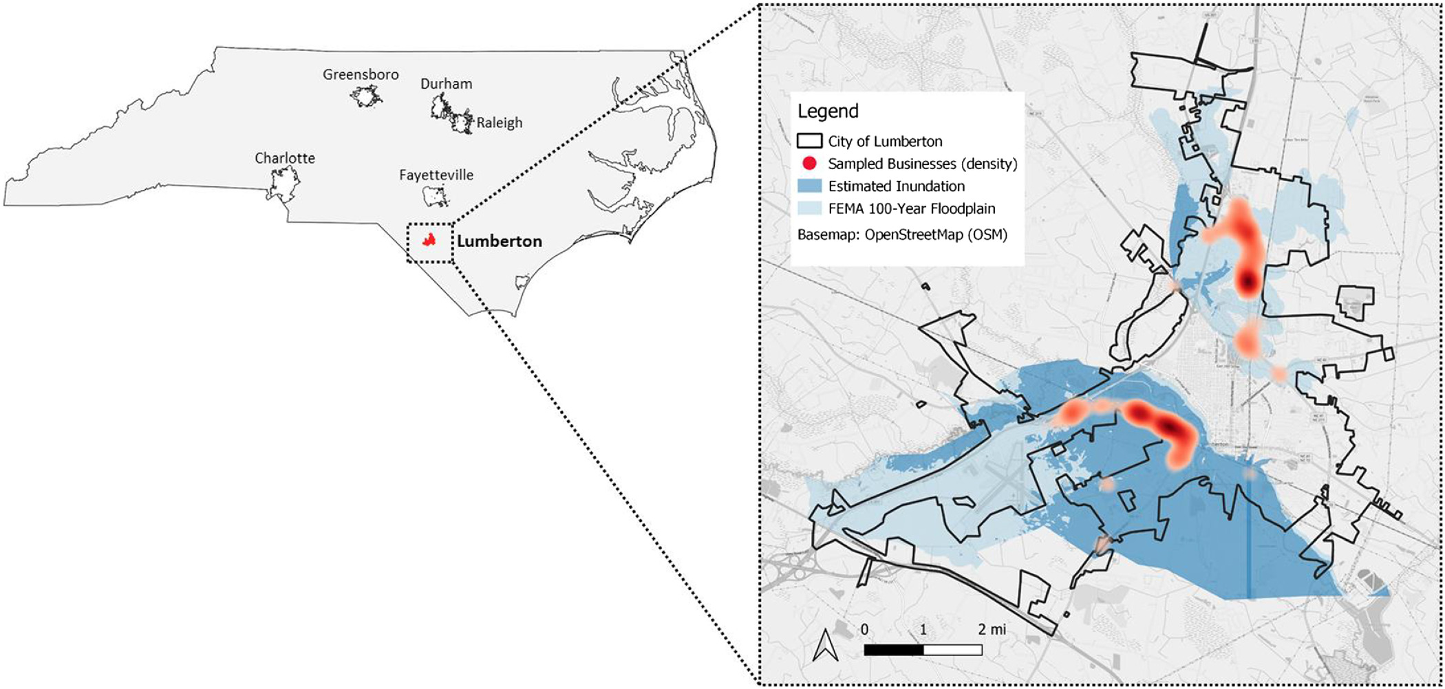
In particular, Lumberton (population. approximately 21,000) was severely impacted by Hurricane Matthew and the resulting heavy rains. The Lumber River that bisects Lumberton experienced a historic flood crest of 6.7 m (22 ft) on October 9—1.2 m (4 ft) higher than the previous maximum flood level, set in 2004 (USGS 2018). Much of the area south of the river was flooded, as were some isolated areas in the northern part of the city (North Carolina Emergency Management 2017). In addition to the inundation of buildings, several utilities were disrupted. Electric power was disrupted due to downed trees and substation flooding, and Lumberton’s sole water treatment plant also was inundated. A boil water advisory was in effect for slightly more than 1 week after service resumed (van de Lindt et al. 2018). Although the flooding was more severe for businesses in the southern commercial corridors, the utility disruption was experienced by businesses across Lumberton. The river receded to below flood stage [4 m (13 ft)] by about October 23 (USGS 2018).
Sample and Data Collection
The business survey effort was part of a larger interdisciplinary effort and longitudinal field study in Lumberton (van de Lindt et al. 2018, 2020; Sutley et al. 2021). The authors used a phone-verified business database downloaded from ReferenceUSA (now Data Axle Reference Solutions) for the sample frame. An inundation shapefile that was created at the University of Alabama through modeling that combined a digital elevation model and the hydrograph from the stream gauge in Lumberton (USGS 02134170) was used in the sample generation: all 218 businesses that were within the inundation area or a 100-m buffer were included, in addition to a random sample of businesses in the 100-year floodplain north of the Lumber River, to obtain to a total of 380 businesses. A map of the sample and study area is presented in Fig. 1. To protect the privacy of individual respondents, the sample is displayed as a heat map of the density of individual businesses.
The survey data were collected through in-person visits to the businesses in January 2018, about 15 months after Hurricane Matthew. The survey instrument was deliberately brief (two pages front and back) and asked businesses questions related to their damage and operations, business characteristics, recovery status, financial assistance, and owner or manager demographics. Survey questions were informed by a systematic review of the business and disaster literature, and were modified from previous business survey efforts if possible (Xiao and Peacock 2014; Xiao et al. 2018). Prior to use in the field, the survey was subjected to a comment period by an interdisciplinary group of researchers at NIST and the NIST-funded Center for Risk-Based Community Resilience Planning.
Questions about the business’s damage corresponded to damage states developed by a team of engineers on the project. These ranged from DS0 to DS4 for building structural damage, content and inventory damage, and machinery and equipment damage. These damage states generally are no damage (DS0), minor damage (DS1), moderate damage (DS2), severe damage (DS3), and complete damage (DS4). The damage states and survey instrument have been published on DesignSafe for reference (Xiao et al. 2020).
Survey teams were multidisciplinary, and had at least one engineer to assist businesses in categorizing their damage in the field; laminated description sheets of each damage state were given to the business to review during the survey. Managers, owners, and employees with enough knowledge to be able to answer questions on the financial decisions of the business were asked to complete the survey. If no one was available at the time of the initial survey team visit, teams scheduled follow-up visits, left a paper survey, or followed-up with phone calls after field deployment. Of the 380 businesses that were sampled, the authors received 164 survey responses, a response rate of 43%, with a sector distribution that matched the Lumberton business population. More detailed information on the sampling strategy and survey methodology were presented by Sutley et al. (2021).
Analytical Methods
This study used closure to measure business interruption. Although businesses can remain partially open and experience interruption losses, many studies have operationalized business interruption as closure, or have used initial closure as a key business resilience metric (Chang and Falit-Baiamonte 2002; Orhan 2014; Ortiz et al. 2021; Sultana et al. 2018). This paper used three approaches to explore how variable choice, variable measurement, and time dynamics affected interruption modeling in the Lumberton case. First, we regressed interruption—i.e., days of closure—on a comprehensive set of damage and utility variables commonly used in descriptive studies, but less common in statistical models. We also did this for sets of control variables, to inform model selection and establish a baseline full model for comparison with the literature. All analyses followed the general formwhere Y = dependent variable, in this case interruption days; is the intercept; is the regression or slope coefficient for the th independent variable, ; and is an error term. Independent variables damage indicators, utility disruption indicators, and other control variables are described in more detail in the next section. For reporting purposes, beta coefficients were translated to percentage change in using
(1)
(2)
Second, we examined how correlation, significance, and model fit was affected by different measures of damage and utility variables, and updated the full model with the controls. Lastly, we recoded the days of interruption dependent variable to represent binary open or closed status at weekly intervals, and ran correlations with the different damage, utility, and control variables to determine how variable relationships change when time is considered for both the dependent and independent variables.
Survey weights were used in the analysis because businesses in the sample had different probabilities of being selected depending on whether they were in the predicted inundation area. Therefore, the study used probability weights (), where is the number of businesses in the population, and is the number of sample businesses, to ensure that the coefficients were not biased. This was done for each regression using the survey design commands in Stata version 17 (StataCorp 2021); although the number of observations may vary, they were all adjusted by a probability weight to represent a consistent population of 508. To facilitate analysis, the damage states were transformed into damage percentages ranging from 0% to 100% (Xiao and Peacock 2014) where Damage states 0–4 were recoded into 0%, 25%, 50%, 75%, and 100%, respectively. There also were outliers in the interruption and utility variables that exerted a large amount of influence on the regression analyses. Therefore, log transformations were used for days of interruption as the dependent variable and days of utility disruptions as independent variables. To preserve zeros in the data, a constant value of 1 was added to all values of the variable before taking the log. Lastly, because damage and utility losses are all related to hazard severity, the variance inflation factor (VIF) of the variables was checked after running each model to identify issues of multicollinearity. The highest VIFs were 3.09 and 2.99, for percentage machinery damage and percentage building damage, in the final full model (Model 22). Although there is no standard threshold, these were below most rule-of-thumb values used to identify cause for concern (James et al. 2013).
Findings
Descriptive Statistics
Descriptive statistics of the sample are presented in Table 2. Almost 40% of businesses in the sample were in the retail or wholesale sector, and 7% were in manufacturing or construction. About 30% were a branch of a larger firm, and about half rented their premises. The size of businesses, measured by number of part- and full-time employees, in the sample ranged from 1 to 250 employees, with an average of 16 at a given facility. Owners, managers, and senior employees who were interviewed had an average of 16 years of business experience, and 40% identified as other than non-Hispanic White.
| Variable | Observationsa | Meanb | Standard deviationb | Min | Max |
|---|---|---|---|---|---|
| Dependent variables | |||||
| Business interruption (days) | 163 | 17.50 | 38.14 | 0 | 300 |
| Business interruption (log days) | 163 | 2.35 | 1.36 | 0 | 5.71 |
| Open at 1 week (1 = yes, 0 = no) | 163 | 0.45 | 0.50 | 0 | 1 |
| Open at 2 weeks (1 = yes, 0 = no) | 163 | 0.71 | 0.46 | 0 | 1 |
| Open at 3 weeks (1 = yes, 0 = no) | 163 | 0.81 | 0.39 | 0 | 1 |
| Open at 4 weeks (1 = yes, 0 = no) | 163 | 0.85 | 0.35 | 0 | 1 |
| Open at 5 weeks (1 = yes, 0 = no) | 163 | 0.90 | 0.30 | 0 | 1 |
| Open at 6 weeks (1 = yes, 0 = no) | 163 | 0.91 | 0.29 | 0 | 1 |
| Damage | |||||
| Building damage: (1 = yes, 0 = no) | 162 | 0.36 | 0.48 | 0 | 1 |
| Content damage: (1 = yes, 0 = no) | 162 | 0.41 | 0.49 | 0 | 1 |
| Machinery or equipment damage: (1 = yes, 0 = no) | 161 | 0.15 | 0.35 | 0 | 1 |
| Building damage (%) | 162 | 16.62 | 34.59 | 0 | 100 |
| Content damage (%) | 162 | 28.25 | 41.09 | 0 | 100 |
| Machinery or equipment damage: (%) | 161 | 10.13 | 26.79 | 0 | 100 |
| Utility disruptions | |||||
| Electricity loss (1 = yes, 0 = no) | 161 | 0.98 | 0.14 | 0 | 1 |
| Water loss (1 = yes, 0 = no) | 161 | 0.91 | 0.28 | 0 | 1 |
| Natural gas loss (1 = yes, 0 = no) | 149 | 0.08 | 0.27 | 0 | 1 |
| Sewer loss (1 = yes, 0 = no) | 153 | 0.36 | 0.48 | 0 | 1 |
| Cell phone service loss (1 = yes, 0 = no) | 158 | 0.30 | 0.46 | 0 | 1 |
| Electricity loss (log days) | 158 | 1.85 | 0.68 | 0 | 5.20 |
| Water loss (log days) | 154 | 2.18 | 0.94 | 0 | 5.20 |
| Natural gas loss (log days) | 148 | 0.20 | 0.79 | 0 | 5.90 |
| Sewer loss (log days) | 146 | 0.83 | 1.37 | 0 | 6.17 |
| Cell phone service loss (log days) | 160 | 0.50 | 0.95 | 0 | 5.48 |
| Transportation disruption | |||||
| Accessibility problem (i.e., street or sidewalk closure): (1 = yes, 0 = no) | 153 | 0.48 | 0.50 | 0 | 1 |
| Customer issues | |||||
| Lost customers (1 = yes, 0 = no) | 161 | 0.61 | 22.92 | 0 | 1 |
| Employee issues | |||||
| Employee home repair problem: (1 = yes, 0 = no) | 154 | 0.51 | 0.50 | 0 | 1 |
| Employee childcare or school problems: (1 = yes, 0 = no) | 157 | 0.25 | 0.43 | 0 | 1 |
| Employee physical or mental health problems: (1 = yes, 0 = no) | 156 | 0.07 | 0.25 | 0 | 1 |
| Business characteristics | |||||
| Branch: (1 = yes, 0 = no) | 164 | 0.41 | 0.49 | 0 | 1 |
| Manufacturing or construction sector: (1 = yes, 0 = no) | 164 | 0.07 | 0.26 | 0 | 1 |
| Retail or wholesale sector: (1 = yes, 0 = no) | 164 | 0.39 | 0.49 | 0 | 1 |
| Number of part- and full-time employees before Hurricane Matthew | 163 | 16.20 | 26.91 | 1 | 250 |
| Rents premises: (1 = yes, 0 = no) | 161 | 0.56 | 0.50 | 0 | 1 |
| Business owner or manager profile | |||||
| Race or ethnicity other than non-Hispanic White: (1 = yes, 0 = no) | 159 | 0.39 | 0.49 | 0 | 1 |
| Years of experience | 158 | 15.85 | 12.43 | 0.02 | 70 |
| Insurance coverage | |||||
| Had building insurance: (1 = yes, 0 = no) | 121 | 0.65 | 0.48 | 0 | 1 |
| Had contents insurance: (1 = yes, 0 = no) | 125 | 0.58 | 0.50 | 0 | 1 |
| Had interruption insurance: (1 = yes, 0 = no) | 113 | 0.34 | 0.47 | 0 | 1 |
a
Descriptive statistics have been weighted to represent the population (). This number represents the number of survey responses associated with the variable.
b
Weighted mean and standard deviation.
In terms of impacts from Hurricane Matthew, businesses in Lumberton were interrupted (i.e., closed for business) for 17 days, on average; the maximum length of interruption was 300 days. By 1 week postflooding, only 45% of businesses in Lumberton had reopened. This percentage rose to 71% after 2 weeks and to 85% after 4 weeks. After 6 weeks, most (91%) of businesses had reopened.
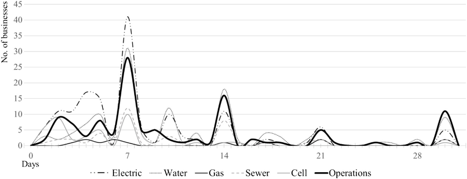
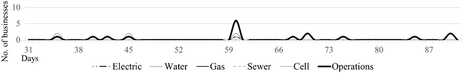
In general, more businesses experienced contents damage (11%) than building (36%) or machinery (15%) damage. Businesses also were more likely to report higher damage levels for their contents than for their building or machinery; businesses reported 17% and 10% damage for their building and machinery, but 25% damage for contents. Content loss can be related to utility loss, and almost all businesses in Lumberton lost electricity and water. Whereas only 12% lost natural gas, 38% lost sewer, and 28% lost cell phone service, 98% lost electricity at some point, and 91% lost water. Figs. 2 and 3 illustrate the restoration of utilities and operations over time during the first 90 days. Most businesses regained their utilities and operations in the first few weeks after the flooding. Businesses waited the longest time to resume service for water; respondents cited an average of close to 12 days without water access. Sewer loss was similar, with an average of almost 12 days with no service. Electricity, natural gas, and telecommunications were disrupted for an average of approximately 7, 3, and 4 days, respectively. However, there were outliers of businesses experiencing very long down times for these services, and some businesses had not had the utility restored at the time of the survey.
Beyond the more physical impacts of Hurricane Matthew, businesses also experienced a variety of impacts related to customers, employees, and their ability to work at and access the business. Approximately 48% of businesses experienced accessibility issues related to street and sidewalk closure, and 61% experienced a loss of customers. Employees were likely to be unable to come to work due personal home damage (50% of businesses). Issues related to childcare and schooling caused employees to be unable to come to work in approximately 25% of businesses, and health problems caused staffing disruption in approximately 7% of the business sample.
Businesses in Lumberton had a variety of insurance coverage types to deal with the flooding impacts. Building insurance was the most commonly held insurance, with 65% of businesses reported having coverage. Content insurance was the second most common, with 58% of businesses in the sample maintaining coverage. Only 34% of businesses had insurance for business interruption. Insurance variables had the highest number of missing values out of the various variables categories. This was due both to managers being unaware of the types of coverage the company had, and to a higher unwillingness to share financial information with the survey team compared with other types of questions. Therefore, we anticipate that these numbers likely were higher because businesses were more likely in the field to respond that they did not know (coded as missing) unless they were sure they had coverage.
Variable Inclusion Considerations
The first set of analyses tested how empirical models of business interruption may be improved through the inclusion of more-comprehensive damage and utility variables used in more-descriptive studies. Table 3 presents a series of models regressing days of interruption on variable groupings of damage and utilities, in addition to transportation, customer, employee, business characteristic, owner or manager profile, and insurance variables that frequently have been used in past studies (Table 1).
| Variable | Model 1 | Model 2 | Model 3 | Model 4 | Model 5 | Model 6 | Model 7 | Model 8 | Model 9 |
|---|---|---|---|---|---|---|---|---|---|
| Coefficient | Coefficient | Coefficient | Coefficient | Coefficient | Coefficient | Coefficient | Coefficient | Coefficient | |
| Constant | 1.522 | 1.692 | 1.552*** | 1.487*** | 2.243*** | 2.229*** | 1.715*** | 2.141*** | 1.283 |
| Damage indicator | |||||||||
| Building (1/0) | 0.151*** | — | — | — | — | — | — | — | 0.153 |
| Contents (1/0) | 0.705*** | — | — | — | — | — | — | — | 0.507** |
| Machinery (1/0) | 1.283*** | — | — | — | — | — | — | — | 0.980*** |
| Utility loss indicator | |||||||||
| Electricity (1/0) | — | — | — | — | — | — | — | ||
| Water (1/0) | — | 0.187 | — | — | — | — | — | — | |
| Gas (1/0) | — | 1.781*** | — | — | — | — | — | — | 1.092*** |
| Sewer (1/0) | — | 0.158 | — | — | — | — | — | — | |
| Cell phone (1/0) | — | — | — | — | — | — | — | ||
| Transportation disruption | |||||||||
| Access | — | — | 1.134*** | — | — | — | — | — | 0.498** |
| Customer issues | |||||||||
| Customers | — | — | — | 0.748*** | — | — | — | — | 0.591*** |
| Employee issues | |||||||||
| Home damage | — | — | — | — | — | — | — | — | |
| Childcare or school | — | — | — | — | 0.078 | — | — | — | — |
| Health | — | — | — | — | 0.882 | — | — | — | — |
| Business characteristics | |||||||||
| Branch | — | — | — | — | — | — | — | — | |
| Manufacturing or construction | — | — | — | — | — | — | — | — | |
| Retail | — | — | — | — | — | — | — | — | |
| No. of employees | — | — | — | — | — | 0.001 | — | — | — |
| Renter | — | — | — | — | — | — | — | — | |
| Owner or manager profile | |||||||||
| Race | — | — | — | — | — | — | 0.235 | — | — |
| Experience | — | — | — | — | — | — | 0.014 | — | — |
| Insurance coverage | |||||||||
| Building | — | — | — | — | — | — | — | 0.256 | — |
| Contents | — | — | — | — | — | — | — | — | |
| Interruption | — | — | — | — | — | — | — | — | |
| 20.79 | 3.63 | 32.58 | 11.94 | 0.86 | 0.79 | 1.82 | 0.80 | 7.70 | |
| -value | 0.000 | 0.004 | 0.000 | 0.001 | 0.464 | 0.557 | 0.165 | 0.498 | 0.000 |
| 0.345 | 0.146 | 0.192 | 0.083 | 0.033 | 0.028 | 0.025 | 0.019 | 0.460 | |
| Sample (before weighting) | 159 | 131 | 153 | 161 | 152 | 150 | 157 | 107 | 118 |
Note: Coefficient = beta coefficient; *; **; and ***.
Models using damage and utility variables were able to explain more of the variation in the (log) number of days a business was closed than were models using other variable categories. Model 1, which included indicators of building, content, and machinery damage, had an value of 0.345. All three types of damage were significantly and positively related to length of business interruption in the Lumberton case. Businesses that experienced building damage, contents damage, and machinery damage were closed for 18%, 3%, and 261% more days, respectively, than businesses that did not report that type of damage. Model 2, which included indicators of electricity, water, natural gas, sewer, and cell phone service outages, had an value of 0.146. Natural gas loss was the only individually significant variable. Businesses experiencing gas loss were interrupted for 493% more days than those without gas loss.
Models 3 and 4, which included transportation disruption and customer loss indicators, also had significant variables. Businesses that experienced accessibility issues with respect to road and sidewalk closure were closed for 211% more days than businesses that did not experience accessibility issues. Similarly, businesses that lost customers were closed for 111% more days than businesses without customer loss. Models 3 and 4, which included access loss and customer loss alone, had values of 0.146 and 0.083, respectively. However, models using business characteristic variables, owner or manager profile variables, and insurance coverage variables did not have any individually significant variables, and the models were insignificant, taken as a whole.
Model 9 was the full model, and included variables in all models with significant -tests (Models 1–4). All utility variables were included from Model 2, despite only natural gas being significant, because many utilities, such as water and sewer, are interdependent. The significance and model fit of each individual utility variable is explored further in the following section. The significance of the individual variables did not change in the full model, with the exception of building damage, which changed from significant in Model 1 to insignificant in Model 9. Contents damage, machinery damage, natural gas loss, access loss, and customer loss all significantly increased interruption duration for Lumberton businesses. The significance of contents and machinery damage compared with building damage highlights the importance of including multiple dimensions of damage in business disruption models, and natural gas loss is rarely if ever included in empirical models. However, including these variables led to the final model having an value of 0.460.
Variable Measurement Considerations
The previous set of analyses showed the importance of including multiple dimensions of damage and utility disruptions, even if only by using binary indicators. However, these variables can be measured and quantified in many ways. For example, surveys can collect detailed information such as days of downtime and level of damage based on damage states. Secondly, given the interdependence of some of the utility provisions and the likelihood that damage severity is related across different physical assets of the business, it is possible that knowing the maximum damage state and days of utility loss across these variables would be sufficient. Therefore the following sets of models explore variable measurements of damage and utilities on interruption, comparing dichotomous measures for damaged–undamaged and lost service–had service with damage state and service disruption duration. Table 4 presents the correlation and the beta coefficient, -value, and model for models regressing days of interruption on each variable individually.
| Variable | Correlation, | Simple linear regression coefficient | |
|---|---|---|---|
| Building damage () | |||
| Percentage (based on damage state) | 0.518*** | 0.022*** | 0.268 |
| Indicator (1 = damaged, 0 = not damaged) | 0.339*** | 0.896*** | 0.115 |
| Contents damage () | |||
| Percentage (based on damage state) | 0.429*** | 0.017*** | 0.280 |
| Indicator (1 = damaged, 0 = not damaged) | 0.472*** | 1.205*** | 0.223 |
| Machinery damage () | |||
| Percentage (based on damage state) | 0.584*** | 0.026*** | 0.300 |
| Indicator (1 = damaged, 0 = not damaged) | 0.522*** | 1.850*** | 0.273 |
| Electricity loss () | |||
| Duration of outage (log days) | 0.513*** | 0.969*** | 0.263 |
| Indicator (1 = lost, 0 = not lost) | 0.021 | 0.198 | 0.000 |
| Water loss () | |||
| Duration of outage (log days) | 0.276*** | 0.375*** | 0.076 |
| Indicator (1 = lost, 0 = not lost) | 0.059 | 0.260 | 0.003 |
| Gas loss () | |||
| Duration of outage (log days) | 0.343*** | 0.586*** | 0.118 |
| Indicator (1 = lost, 0 = not lost) | 0.357*** | 1.765*** | 0.127 |
| Sewer loss () | |||
| Duration of outage (log days) | 0.238** | 0.224*** | 0.056 |
| Indicator (1 = lost, 0 = not lost) | 0.096 | 0.264 | 0.009 |
| Cell loss () | |||
| Duration of outage (log days) | 0.158 | 0.214 | 0.025 |
| Indicator (1 = lost, 0 = not lost) | 0.001 | 0.001 | 0.000 |
| Maximum disruption (, ) | |||
| Maximum damage state (DS1–DS5) | 0.528*** | 0.016*** | 0.261 |
| Maximum utility loss (log days) | 0.566*** | 0.566*** | 0.179 |
Note: Coefficient = beta coefficient from simple regression model; *; **; and ***.
The results in Table 4 suggest that interruption models are sensitive to more-imprecise measurements in utility disruption, but comparatively less so for damage. For example, the weighted correlations between damage variables and log days of interruption and the beta coefficients when using each damage variable in a simple regression model with log days of interruption were significant regardless of whether the percentage damage based on damage state or binary measure was used. However, for utility disruption, using log days instead of the binary measure led to changes in significance in both the correlations and the beta coefficients in the case of electricity, water, and sewer loss. Whereas the binary measure was insignificant in these cases, the log days of disruption to those utilities was significantly related to log days of interruption. For natural gas and cell phone loss, both the binary and continuous measures were significant and insignificant, respectively.
Across the damage and utility variables, the value generally was higher when percentage damage and log days of utility outages were used in the simple regression models. This was most pronounced for building damage and electricity loss. For building damage, a simple regression model using the binary measure had an value of 0.115, whereas a simple regression model using percentage damage based on the damage state had an value of 0.268. For electricity loss, the difference was greater: a simple regression model using the binary measure had an value of , whereas a simple regression model using the duration of electricity loss had an value of 0.263. However, the values cannot be compared directly.
Tables 5 and 6 present the result of using continuous measures in place of the indicator variables, using partial -tests to determine whether these additions can improve the value significantly. Adding more-precise measures of utility disruption significantly improved the in Table 5, whereas using the indicator measures did not. The value increased by 0.107 in Model 12 (, ) and 0.083 in Model 15 (, ) when adding log days of utility loss and increased by 0.061 in Model 11 (, ) and 0.039 in Model 14 (, ) when adding the indicator measures. Adding the percent damage variables and damage indicator measures both significantly improved the value in Table 6. The value increased by 0.294 in Model 18 (, ) and by 0.162 in Model 21 (, ) when adding percentage damage, and it increased by 0.239 in Model 17 (, ) and by 0.109 (, ) when adding the indicator measures. Overall, the results suggest that adding nonbinary variables can increase the model goodness-of-fit more than adding the binary variables. It also changed the significance of some of the variables: both electricity loss and building damage gained significance when using days of utility loss and percentage damage, respectively.
| Variable | Model 10 (restricted) | Model 11 (unrestricted) | Model 12 (unrestricted) | Model 13 (restricted) | Model 14 (unrestricted) | Model 15 (unrestricted) |
|---|---|---|---|---|---|---|
| Coefficient | Coefficient | Coefficient | Coefficient | Coefficient | Coefficient | |
| Constant | 1.494 | 1.371 | 0.428 | 1.483 | 0.526 | — |
| Damage indicator | ||||||
| Building (1/0) | 0.194 | 0.165 | 0.128 | — | — | — |
| Contents (1/0) | 0.644** | 0.655*** | 0.504** | — | — | — |
| Machinery (1/0) | 1.351*** | 1.135*** | 0.825** | — | — | — |
| Percentage damage (%) | ||||||
| Building | — | — | — | 0.010*** | 0.010*** | 0.009*** |
| Contents | — | — | — | 0.008*** | 0.008*** | 0.006** |
| Machinery) | — | — | — | 0.012*** | 0.010*** | 0.007** |
| Utility loss indicator | ||||||
| Electricity (1/0) | — | 0.032 | — | — | 0.139 | — |
| Water (1/0) | — | 0.115 | — | — | 0.162 | — |
| Gas (1/0) | — | 1.209*** | — | — | 0.970** | — |
| Sewer (1/0) | — | — | — | — | ||
| Cell (1/0) | — | — | — | — | ||
| Log days of utility loss | ||||||
| Electricity (log days) | — | — | 0.453** | — | — | 0.435** |
| Water (log days) | — | — | 0.113 | — | — | 0.126 |
| Gas (log days) | — | — | 0.271** | — | — | 0.189 |
| Sewer (log days) | — | — | 0.023 | — | — | |
| Cell (log days) | — | — | 0.094 | — | — | 0.087 |
| 14.19 | 7.99 | 13.10 | 30.00 | 12.71 | 15.85 | |
| -value | 0.000 | 0.000 | 0.000 | 0.000 | 0.000 | 0.000 |
| 0.320 | 0.381 | 0.427 | 0.397 | 0.436 | 0.480 | |
| Change in | — | 0.061 | 0.107 | — | 0.039 | 0.083 |
| Partial -statistic | — | 1.63 | 3.92 | — | 1.13 | 3.14 |
| Partial -statistic -value | — | 0.157 | 0.003 | — | 0.349 | 0.011 |
| sample (before weighting) | 127 | 127 | 127 | 127 | 127 | 127 |
Note: coefficient = beta coefficient; *; **; and ***.
| Variable | Model 16 (restricted) | Model 17 (unrestricted) | Model 18 (unrestricted) | Model 19 (restricted) | Model 20 (unrestricted) | Model 21 (unrestricted) |
|---|---|---|---|---|---|---|
| Coefficient | Coefficient | Coefficient | Coefficient | Coefficient | Coefficient | |
| Constant | 1.655 | 1.371 | 0.526 | 0.157 | 0.428 | — |
| Utility loss indicator | ||||||
| Electricity (1/0) | 0.020 | 0.032 | 0.139 | — | — | — |
| Water (1/0) | 0.187 | 0.115 | 0.162 | — | — | — |
| Gas (1/0) | 1.746*** | 1.209*** | 0.970** | — | — | — |
| Sewer (1/0) | 0.090 | — | — | — | ||
| Cell (1/0) | — | — | — | |||
| Log days of utility loss | ||||||
| Electricity (log days) | — | — | — | 0.691*** | 0.453** | 0.435 |
| Water (log days) | — | — | — | 0.159 | 0.113 | 0.126 |
| Gas (log days) | — | — | — | 0.367*** | 0.271** | 0.189 |
| Sewer (log days) | — | — | — | 0.087 | 0.023 | |
| Cell (log days) | — | — | — | 0.118 | 0.094 | 0.087 |
| Damage indicator | ||||||
| Building (1/0) | — | 0.165 | — | — | 0.128 | — |
| Contents (1/0) | — | 0.655*** | — | — | 0.504** | — |
| Machinery (1/0) | — | 1.135*** | — | — | 0.825** | — |
| Percentage damage (%) | ||||||
| Building | — | — | 0.010*** | — | — | 0.009*** |
| Contents | — | — | 0.008*** | — | — | 0.006** |
| Machinery | — | — | 0.010*** | — | — | 0.007** |
| 3.15 | 7.99 | 12.71 | 12.77 | 13.10 | 15.85 | |
| -value | 0.010 | 0.000 | 0.000 | 0.000 | 0.000 | 0.000 |
| 0.142 | 0.381 | 0.436 | 0.318 | 0.427 | 0.480 | |
| Change in | — | 0.239 | 0.294 | — | 0.109 | 0.162 |
| Partial -statistic | — | 15.05 | 26.29 | — | 5.20 | 12.56 |
| Partial -statistic -value | — | 0.000 | 0.000 | — | 0.002 | 0.000 |
| Sample (before weighting) | 127 | 127 | 127 | 127 | 127 | 127 |
Note: Coefficient = beta coefficient; *; **; and ***.
Lastly, the bottom two rows in the Table 4 present the interruption correlations and simple regression results with the maximum percentage damage across the building, machinery, and contents, and the longest (logged) days of utility outage across electricity, water, gas, sewer, and cell phone service for each business. The values were 0.18 and 0.27 for maximum damage and maximum utility outage duration, respectively. These measures may be an efficient alternative for smaller samples, because they use only one degree of freedom.
Time Considerations
The analysis in the section titled “Variable Measurement Considerations” displayed the particular importance of examining utility outage durations rather than basic indicators when modeling business interruption, and indicate that there is some relationship between utilities, closure, and time. Additionally, the significance of individual utilities is different depending on whether the duration or indicator measure was used. Therefore the final analysis explored this more deeply by examining how variable measures behave over time (Table 7). Business interruption was measured using binary indicators in previous studies (see Table 1); therefore, this analysis explores the importance of capturing time in both dependent and independent variables.
| Variable | Open at 1 week (45% of sampled businesses open) | Open at 2 weeks (71% of sampled businesses open) | Open at 3 weeks (81% of sampled businesses open) | Open at 4 weeks (85% of sampled businesses open) | Open at 5 weeks (90% of sampled businesses open) | Open at 6 weeks (91% of sampled businesses open) |
|---|---|---|---|---|---|---|
| Building (1/0) | *** | *** | *** | *** | *** | *** |
| Contents (1/0) | *** | *** | *** | *** | *** | *** |
| Machinery (1/0) | *** | *** | *** | *** | *** | *** |
| Building (%) | *** | *** | *** | *** | *** | *** |
| Contents (%) | *** | *** | *** | *** | *** | *** |
| Machinery (%) | *** | *** | *** | *** | *** | *** |
| Electric (initial) | 0.005 | 0.042 | 0.065 | 0.098 | 0.104 | |
| Water (initial) | 0.020 | 0.072 | 0.080 | |||
| Gas (initial) | ** | *** | ** | ** | *** | *** |
| Sewer (initial) | 0.009 | 0.014 | ||||
| Cell (initial) | 0.066 | 0.045 | 0.029 | 0.003 | ||
| Electric (in period) | *** | *** | *** | ** | ||
| Water (in period) | ** | ** | *** | * | ||
| Gas (in period) | *** | *** | ** | ** | ** | ** |
| Sewer (in period) | ** | ** | ** | ** | * | |
| Cell (in period) | ||||||
| Customer loss (%) | * | * | * | * | * | |
| Access | *** | *** | *** | *** | *** | *** |
Note: *; **; and ***.
The days of interruption variable was used to create a series of binary indicators for whether the business had reopened each week, starting from Week 1 and ending at Week 6, at which time most (91%) of the sample had resumed their operations. Days of utility outage information was recoded to create a series of binary indicators for whether the business had that particular utility restored in the same periods (denoted “in period” in Table 7). These variables were included along with the initial binary loss measure for the utilities, the binary measure for damage, the damage state measures, customer loss, and access loss used in previous analyses.
The results in Table 7 further support the conclusions presented in the “Variable Measurement Considerations” section and clarify some of the variable significance discrepancies. The percentage damage measures had greater correlations with business reopening at all time periods than did the damage indicator measures. However, the biggest differences involved the utility loss measures. Natural gas was the only variable that was significantly correlated with reopening across the different periods when considering only the initial utility loss, which corroborates its significance in the first full model (Model 9). However, examining utility restorations in the different periods indicates that all the utility services except cell phone service were significantly correlated with business reopening in one or more periods. The correlations also indicate how the effects of the utilities differed depending on the time since the initial flooding, and likely capture different rates of restoration. Electricity had a very high correlation with reopening in the first few weeks, but became insignificant at 5 weeks. Conversely, sewer and gas had stronger correlations in later weeks than in earlier weeks. Some businesses experienced very long disruptions to these utilities in particular, as indicated by the high maximum values and standard deviations in Table 2. It is possible that certain utilities became the limiting factor to reopening as time went on, even as other utilities were restored. This is supported by the value of 0.179 for the model that used the maximum utility loss variable alone (Table 3) and the chart of reopenings and utility restorations after Day 30 (Fig. 2).
The final interruption model is presented in Table 8. This model included all variables significantly related to interruption (Table 3) and the measurement improvements in the dependent and independent variables explored in Tables 4–7. In the final model, building damage, machinery damage, electricity loss, access loss, and customer loss were significantly associated with length of interruption. For each additional percentage of building damage and machinery damage, businesses were interrupted for 1% and 0.7% more days, respectively, controlling for all other variables. For each additional 1% increase in days of electricity loss, businesses were interrupted for 42% more days, controlling for other variables. Finally, businesses experiencing customer loss and access loss were interrupted for 62% and 55% more days, respectively, controlling for damage and utility losses. Although contents damage was significant in previous models, the -value for this variable was 0.120 in the final model using a two-tailed test. Although this approached significance at the 0.1 level, it ultimately was insignificant. Altogether, variables in the final model were able to explain approximately 54% of the variation in (log) interruption days.
| Variable | Model 22 |
|---|---|
| Coefficient | |
| Constant | 0.182 |
| Percentage damage (%) | |
| Building | 0.010*** |
| Contents | 0.004 |
| Machinery | 0.007** |
| Log days of utility loss | |
| Electricity (log days) | 0.351* |
| Water (log days) | 0.105 |
| Gas (log days) | 0.135 |
| Sewer (log days) | |
| Cell (log days) | 0.145 |
| Transportation disruption | |
| Access | 0.435** |
| Customer issues | |
| Customers | 0.483*** |
| 12.00 | |
| -value | 0.000 |
| 0.542 | |
| Sample (before weighting) | 118 |
Note: Coefficient = beta coefficient; *; **; and ***.
Discussion and Conclusions
In this paper we explored how to use survey data efficiently and effectively in business interruption models after disasters through analysis of variable choice, variable measurement, and measurement timing. We found that including more comprehensive damage and utility variables, even simple binary loss measures, could improve empirical models. However, the way in which damage and utilities were measured also made a difference in model fit: across the damage and utility variables, the value generally was higher when damage states and log days of disruption were used in regression models, compared with using the indicator or binary measures. Utility variables were particularly sensitive to measurement changes. Examining whether a business lost utility services using only a binary measure, only natural gas was significant. However, when accounting for time, either through days of outage or whether the service was restored at different points in recovery, only cell phone service was not significantly related to closure. Therefore, using different measures can lead to a different conclusion about which utility service is most important.
In particular, we found that the correlations with reopening were stronger for different utilities depending on the number of weeks after the event, and the maximum number of days lost for any utility was a fairly efficient measure by itself. These findings are not entirely surprising considering that recovery is a dynamic process—and flow measures have been said to be superior to stock measures when modeling business interruption losses after disasters—but they have very practical implications for survey design. Businesses were reopening and different utilities were being restored on a daily basis, especially early on (Figs. 1 and 2). It follows that the better a survey can capture recovery dynamics through time, the better it will be able to capture the process of business interruption and reopening. Damage varied less across types of measurement because it is measuring an initial state condition; having more information in terms of the engineering damage states was beneficial in terms of model fit, but comparatively less so. Utility restoration is very dynamic, and more-substantial improvements can be gained when considering duration of outages rather than whether the outage occurred. Asking businesses about days of utility loss rather than whether they lost service is an easy survey modification. Although it is unlikely to add to the response burden of the survey, it can make a great difference in the resulting analysis.
Survey development is important for facilitating interdisciplinary collaboration, building better models, and supporting more-ethical research practices. We believe that the types of analyses presented in this paper can lead to evidence-based survey design for businesses, which will benefit both the researcher and the respondent. Researchers can improve the types of analyses that result from surveys, and the survey burden on disaster-affected respondents may be reduced as questions and measures become more efficient. We support efforts to begin better standardization of survey instruments through open data sharing platforms such as DesignSafe, on which the survey for this study has been published (Xiao et al. 2020). Because Lumberton is a fairly small community and the analysis was limited to flood hazard, publishing, pooling, and contrasting data that have been collected through comparable tools across different hazard types also will advance empirical modeling efforts. These data also can be built upon to calculate interruption losses or can be used as a validation exercise (Rose and Lim 2002). Similarly, survey data can be validated with and compared against engineering models of utility loss. Utility restorations peaked at 7 and 14 days (Fig. 2), which could be reflective of the true restoration times but could also be due to businesses responding “one week” or “two weeks” due to rounding or recall bias. Because the more detailed utility models routinely outperformed the others, this could be an opportunity for further refinement.
Interdisciplinary collaboration and data sharing has a secondary benefit of also allowing refinements to survey design beyond what this paper proposes. This paper quantified the benefit of measuring utility disruptions as flow measures; however, this is likely to extend to other variables. Future surveys could improve upon this research by comparing initial damage states with the restoration process measured in days until full or partial repair. Similarly, other variables such as transportation access or customer loss could be phrased to incorporate the days until they were restored to pre-event levels. The further evaluation of customer and employee loss variables is particularly important given their potential for measurement error. For example, this study assumed that businesses waited to reopen until they knew that their market and employees had returned; however, when responding to the survey, businesses might have referred only to loss of customers after the business had reopened. Further refinements to this survey question likely would yield more-accurate information.
Lastly, in the case of Lumberton, initial business interruption after Hurricane Matthew was highly related to lack of utility service, the physical building, and its contents, rather than business characteristics. This research primarily focused on the first few weeks after an event—because over 90% of businesses in the sample had reopened by Week 6—and previous research has suggested that factors affecting business recovery can change as time progresses (Sydnor et al. 2017; Watson et al. 2020). These variables still should be considered for use in modeling efforts, especially when used in risk-based or community resilience models in which outcomes across different types of businesses can be informative for planning purposes. Still, planners and policymakers interested in business continuity might concentrate on mitigation and preparedness measures aimed at reducing those disruptions in particular for future hurricanes. This could include structural mitigation of the building against flooding, securing offsite storage for inventory, purchasing backup generators, installing backflow valves on drainage systems, and generally exploring ways to become less dependent on the business’s physical location (Xiao and Peacock 2014; Ready Business 2017; Lindell and Perry 1998).
Data Availability Statement
Some or all data, models, or code generated or used during the study are proprietary or confidential in nature and may be provided only with restrictions (e.g., anonymized data). This includes all damage data at a level of detail in which individual businesses can be identified and all business survey data at a level of detail in which individuals and their responses to any survey questions can be identified.
Acknowledgments
The Center for Risk-Based Community Resilience Planning is a NIST-funded Center of Excellence; the Center is funded through a cooperative agreement between the US National Institute of Standards and Technology and Colorado State University (NIST Financial Assistance Award numbers 70NANB15H044 and 70NANB20H008). The views expressed are those of the authors and may not represent the official position of the National Institute of Standards and Technology or the US Department of Commerce.
References
Aghababaei, M., M. Koliou, M. Watson, and Y. Xiao. 2021. “Quantifying post-disaster business recovery through Bayesian methods.” Struct. Infrastruct. Eng. 17 (6): 838–856. https://doi.org/10.1080/15732479.2020.1777569.
Alesch, D. J., J. N. Holly, E. Mittler, and R. Nagy. 2001. Organizations at risk: What happens when small businesses and not-for-profits encounter natural disasters. Fairfax, VA: Public Entity Risk Institute.
Armstrong, T. 2017. “Hurricane Matthew in the Carolinas: October 8, 2016.” National Weather Service. Accessed August 22, 2022. https://www.weather.gov/ilm/Matthew.
Asgary, A., M. I. Anjum, and N. Azimi. 2012. “Disaster recovery and business continuity after the 2010 flood in Pakistan: Case of small businesses.” Int. J. Disaster Risk Reduct. 2 (Dec): 46–56. https://doi.org/10.1016/j.ijdrr.2012.08.001.
Brookshire, D. S., S. E. Chang, H. Cochrane, R. A. Olson, A. Rose, and J. Steenson. 1997. “Direct and indirect economic losses from earthquake damage.” Earthquake Spectra 13 (4): 683–701. https://doi.org/10.1193/1.1585975.
Brown, C., J. Stevenson, S. Giovinazzi, E. Seville, and J. Vargo. 2015. “Factors influencing impacts on and recovery trends of organisations: Evidence from the 2010/2011 Canterbury earthquakes.” Int. J. Disaster Risk Reduct. 14 (Dec): 56–72. https://doi.org/10.1016/j.ijdrr.2014.11.009.
Burrus, R. T., Jr., C. F. Dumas, C. H. Farrell, and W. W. Hall Jr. 2002. “Impact of low-intensity hurricanes on regional economic activity.” Nat. Hazards Rev. 3 (3): 118–125. https://doi.org/10.1061/(ASCE)1527-6988(2002)3:3(118).
Chang, S. E. 2000. “Disasters and transport systems: Loss, recovery and competition at the Port of Kobe after the 1995 earthquake.” J. Transp. Geogr. 8 (1): 53–65. https://doi.org/10.1016/S0966-6923(99)00023-X.
Chang, S. E. 2010. “Urban disaster recovery: A measurement framework and its application to the 1995 Kobe earthquake.” Disasters 34 (2): 303–327. https://doi.org/10.1111/j.1467-7717.2009.01130.x.
Chang, S. E., and A. Falit-Baiamonte. 2002. “Disaster vulnerability of businesses in the 2001 Nisqually earthquake.” Global Environ. Change Part B: Environ. Hazards 4 (2): 59–71. https://doi.org/10.1016/S1464-2867(03)00007-X.
Chang, S. E., W. D. Svekla, and M. Shinozuka. 2002. “Linking infrastructure and urban economy: Simulation of water-disruption impacts in earthquakes.” Environ. Plann. B: Urban Anal. City Sci. 29 (2): 281–301. https://doi.org/10.1068/b2789.
Dahlhamer, J. M., and K. J. Tierney. 1996. Winners and losers: Predicting business disaster recovery outcomes following the Northridge earthquake. Newark, DE: Disaster Research Center, Univ. of Delaware.
Dormady, N., A. Rose, H. Rosoff, and A. Roa-Henriquez. 2019. “Estimating the cost-effectiveness of resilience to disasters: Survey instrument design and refinement of primary data.” In Handbook on resilience of socio-technical systems. Cheltenham, UK: Edward Elgar.
Flott, P. 1997. “An analysis of the determinants of recovery of businesses after a natural disaster using a multi-paradigm approach.” Ph.D. thesis, Dept. of Management, Univ. of North Texas.
James, G., D. Witten, T. Hastie, and R. Tibshirani. 2013. Vol. 112 of An introduction to statistical learning, 18. New York: Springer.
Jiang, X., N. Mori, H. Tatano, L. Yang, and Y. Shibutani. 2016. “Estimation of property loss and business interruption loss caused by storm surge inundation due to climate change: A case of Typhoon Vera revisit.” Supplement, Nat. Hazards 84 (S1): 35–49. https://doi.org/10.1007/s11069-015-2085-z.
Kajitani, Y., and H. Tatano. 2009. “Estimation of lifeline resilience factors based on surveys of Japanese industries.” Earthquake Spectra 25 (4): 755–776. https://doi.org/10.1193/1.3240354.
Khan, M. A. U., and M. A. Sayem. 2013. “Understanding recovery of small enterprises from natural disaster.” Environ. Hazards-Human Policy Dimens. 12 (3–4): 218–239. https://doi.org/10.1080/17477891.2012.761593.
Koliou, M., J. W. van de Lindt, T. P. McAllister, B. R. Ellingwood, M. Dillard, and H. Cutler. 2020. “State of the research in community resilience: Progress and challenges.” Sustainable Resilient Infrastruct. 5 (3): 131–151. https://doi.org/10.1080/23789689.2017.1418547.
Lam, N. S., H. Arenas, K. Pace, J. LeSage, and R. Campanella. 2012. “Predictors of business return in New Orleans after Hurricane Katrina.” PLoS One 7 (10): e47935. https://doi.org/10.1371/journal.pone.0047935.
Lam, N. S., K. Pace, R. Campanella, J. LeSage, and H. Arenas. 2009. “Business return in New Orleans: Decision making amid post-Katrina uncertainty.” PLoS One 4 (8): e6765. https://doi.org/10.1371/journal.pone.0006765.
Lee, J. 2019. “Business recovery from Hurricane Harvey.” Int. J. Disaster Risk Reduct. 34 (Mar): 305–315. https://doi.org/10.1016/j.ijdrr.2018.12.004.
Lindell, M. K., and R. W. Perry. 1998. “Earthquake impacts and hazard adjustment by acutely hazardous materials facilities following the Northridge earthquake.” Earthquake Spectra 14 (2): 285–299. https://doi.org/10.1193/1.1586000.
Marshall, M. I., and H. L. Schrank. 2014. “Small business disaster recovery: A research framework.” Nat. Hazards 72 (2): 597–616. https://doi.org/10.1007/s11069-013-1025-z.
North Carolina Emergency Management. 2017. “Hurricane Matthew resilient redevelopment plan: Robeson County.” Accessed August 22, 2022. https://files.nc.gov/rebuildnc/documents/matthew/rebuildnc_robeson_plan_combined.pdf.
Orhan, E. 2014. “The role of lifeline losses in business continuity in the case of Adapazari, Turkey.” Environ. Hazards-Human Policy Dimens. 13 (4): 298–312. https://doi.org/10.1080/17477891.2014.922914.
Ortiz, D., E. Reinoso, and J. A. Villalobos. 2021. “Assessment of business interruption time due to direct and indirect effects of the Chiapas earthquake on September 7th 2017.” Nat. Hazards 108 (3): 2813–2833. https://doi.org/10.1007/s11069-021-04801-x.
Ready Business. 2017. “Inland flooding toolkit.” Accessed September 6, 2023. https://www.ready.gov/sites/default/files/2020-04/ready_business_inland-flooding-toolkit.pdf.
Rose, A., and C. K. Huyck. 2016. “Improving catastrophe modeling for business interruption insurance needs.” Risk Anal. 36 (10): 1896–1915. https://doi.org/10.1111/risa.12550.
Rose, A., and D. Lim. 2002. “Business interruption losses from natural hazards: Conceptual and methodological issues in the case of the Northridge earthquake.” Global Environ. Change Part B: Environ. Hazards 4 (1): 1–14. https://doi.org/10.1016/S1464-2867(02)00012-8.
Shi, Y., S. Jin, and K. Seeland. 2015. “Modeling business interruption impacts due to disrupted highway network of Shifang by the Wenchuan earthquake.” Nat. Hazards 75 (2): 1731–1745. https://doi.org/10.1007/s11069-014-1391-1.
StataCorp. 2021. Stata survey data reference manual release 17. College Station, TX: StataCorp.
Stewart, S. R. 2017. National Hurricane center tropical cyclone report: Hurricane Matthew. AL142016. Miami: National Oceanic and Atmospheric Administration, National Weather Service, National Hurricane Center.
Sultana, Z., T. Sieg, P. Kellermann, M. Müller, and H. Kreibich. 2018. “Assessment of business interruption of flood-affected companies using random forests.” Water 10 (8): 1049. https://doi.org/10.3390/w10081049.
Sutley, E., M. Dillard, and J. van de Lindt. 2021. Community resilience-focused technical investigation of the 2016 Lumberton, North Carolina Flood: Community recovery one year later. Special Publication (NIST SP). Gaithersburg, MD: NIST.
Sydnor, S., L. Niehm, Y. Lee, M. Marshall, and H. Schrank. 2017. “Analysis of post-disaster damage and disruptive impacts on the operating status of small businesses after Hurricane Katrina.” Nat. Hazards 85 (3): 1637–1663. https://doi.org/10.1007/s11069-016-2652-y.
Tierney, K. J. 1995. Impacts of recent US disasters on businesses: The 1993 Midwest floods and the 1994 Northridge Earthquake. Newark, DE: Disaster Research Center, Univ. of Delaware.
Tierney, K. J. 1997. “Business impacts of the Northridge earthquake.” J. Contingencies Crisis Manage. 5 (2): 87–97. https://doi.org/10.1111/1468-5973.00040.
Tierney, K. J., and J. M. Nigg. 1995. Business vulnerability to disaster-related lifeline disruption. Newark, DE: Disaster Research Center, Univ. of Delaware.
USGS. 2018. “Lumber River at Lumberton, NC-02134170.” Accessed September 6, 2023. https://waterdata.usgs.gov/monitoring-location/02134170/#parameterCode=00065&startDT=2016-10-06&endDT=2016-10-23showMedian=true&startDT=2016-09-28endDT=2016-10-27.
van de Lindt, J. W., et al. 2018. The Lumberton, North Carolina Flood of 2016: A Community resilience focused technical investigation. Special Publication (NIST SP) 1230. Gaithersburg, MD: NIST.
van de Lindt, J. W., et al. 2020. “Community resilience-focused technical investigation of the 2016 Lumberton, North Carolina, flood: An interdisciplinary approach.” Nat. Hazards Rev. 21 (3): 04020029. https://doi.org/10.1061/(ASCE)NH.1527-6996.0000387.
Wang, W. L., M. Watson, J. W. van de Lindt, and Y. Xiao. 2023. “Commercial building recovery methodology for use in community resilience modeling.” Nat. Hazards Rev. 24 (4): 04023031. https://doi.org/10.1061/NHREFO.NHENG-1728.
Wasileski, G., H. Rodríguez, and W. Diaz. 2011. “Business closure and relocation: A comparative analysis of the Loma Prieta earthquake and Hurricane Andrew.” Disasters 35 (1): 102. https://doi.org/10.1111/j.1467-7717.2010.01195.x.
Watson, M., Y. Xiao, J. Helgeson, and M. Dillard. 2020. “Importance of households in business disaster recovery.” Nat. Hazards Rev. 21 (4): 05020008. https://doi.org/10.1061/(ASCE)NH.1527-6996.0000393.
Xiao, Y. et al. 2020 “Business survey instrument, January 19, 2018: Wave 2.” In A longitudinal community resilience focused technical investigation of the Lumberton, North Carolina flood of 2016. Seattle: DesignSafe-CI. https://doi.org/10.17603/ds2-f9kt-fm93 v1.
Xiao, Y., and W. G. Peacock. 2014. “Do hazard mitigation and preparedness reduce physical damage to businesses in disasters? Critical role of business disaster planning.” Nat. Hazards Rev. 15 (3): 04014007. https://doi.org/10.1061/(ASCE)NH.1527-6996.0000137.
Xiao, Y., K. Wu, D. Finn, and D. Chandrasekhar. 2018. “Community businesses as social units in post-disaster recovery.” J. Plann. Educ. Res. 42 (1): 76–89. https://doi.org/10.1177/0739456X18804328.
Yang, L., Y. Kajitani, H. Tatano, and X. Jiang. 2016. “A methodology for estimating business interruption loss caused by flood disasters: Insights from business surveys after Tokai Heavy Rain in Japan.” Nat. Hazards 84 (Nov): 411–430. https://doi.org/10.1007/s11069-016-2534-3.
Information & Authors
Information
Published In

Natural Hazards Review
Volume 25 • Issue 1 • February 2024
Copyright
This work is made available under the terms of the Creative Commons Attribution 4.0 International license, https://creativecommons.org/licenses/by/4.0/.
History
Received: Dec 12, 2022
Accepted: Jul 10, 2023
Published online: Sep 26, 2023
Published in print: Feb 1, 2024
Discussion open until: Feb 26, 2024
ASCE Technical Topics:
- Business management
- Data analysis
- Disaster risk management
- Disasters and hazards
- Economic factors
- Engineering fundamentals
- Field tests
- Hurricanes, typhoons, and cyclones
- Infrastructure
- Lifeline systems
- Measurement (by type)
- Methodology (by type)
- Metric systems
- Natural disasters
- Practice and Profession
- Research methods (by type)
- Social factors
- Tests (by type)
- Utilities
Authors
Metrics & Citations
Metrics
Citations
Download citation
If you have the appropriate software installed, you can download article citation data to the citation manager of your choice. Simply select your manager software from the list below and click Download.