Multispectral Imaging for Identification of High-Water Marks in Postdisaster Flood Reconnaissance

Gardner, Michael; Nichols, Elliot; Stark, Nina; Lemnitzer, Anne; Frost, David

doi:10.1061/NHREFO.NHENG-1735

Open access

Technical Notes

Feb 25, 2023

Multispectral Imaging for Identification of High-Water Marks in Postdisaster Flood Reconnaissance

Authors: Michael Gardner, M.ASCE https://orcid.org/0000-0002-5238-630X [email protected], Elliot Nichols, S.M.ASCE https://orcid.org/0000-0001-7815-0429 [email protected], Nina Stark, A.M.ASCE https://orcid.org/0000-0001-9484-069X [email protected], Anne Lemnitzer, A.M.ASCE https://orcid.org/0000-0001-9866-4726 [email protected], and David Frost, F.ASCE [email protected]Author Affiliations

Publication: Natural Hazards Review

Volume 24, Issue 2

https://doi.org/10.1061/NHREFO.NHENG-1735

PDF

Abstract

Flooding annually causes thousands of fatalities and billions of dollars in damage globally. Predicting future floods has become increasingly challenging due to changing urban environments and land surface conditions. Simultaneously, severe floods are likely to increase due to climate change and associated shifts in rain patterns, resulting into potentially stronger and more consequential flood events. High-water marks represent key information to be collected after flooding for advancing the understanding of flood impacts and the development of mitigation strategies. However, high-water marks often become increasingly difficult to detect with time passing after a flood event due to drying. In addition, access into flooded areas can be complicated by destroyed infrastructure, leading to significant loss of data or risk to personnel entering these recently flooded areas. Here, initial data are presented demonstrating the application of multispectral imagery in rapidly collecting and mapping high-water marks after flooding. The multispectral images were collected 3–4 weeks after the July 14, 2021, western European flood events in the town of Mayschoss, Germany, along the Ahr River. At that time, affected buildings, walls, and soil were exposed to high summer temperatures and solar radiation, as well as dust from surrounding emergency response and repair works. High-water marks were barely visible by eye. Preliminary results showed the high-water mark is significantly enhanced in the blue band (wavelength 443 to 507 nm) and can be modally isolated through linear combination of the blue band and red-edge band (wavelength 705 to 729 nm). The results illustrate the potential to apply this technique in postdisaster reconnaissance to quickly and safely map high-water levels to identify the magnitude and extent of flooding in urban areas.

Introduction

Flooding accounts for 80%–90% of documented natural disasters globally (CRED 2021), causing extensive damage, death, and disruption. The recent 2021 flooding in western Europe serves as a potent example of risks posed by extreme flooding. With over 230 fatalities, the July 14–15, 2021, event was the most destructive flooding Europe has experienced in the 21st century (Statista 2022). Early estimates of flood-related damage suggested approximately 350 million Euros of damage in Belgium (Kreienkamp et al. 2021), 300–600 million Euros in the Netherlands (Jonkman et al. 2021), and 17 billion Euros in Germany (AON 2021). More recent analyses by the German reinsurance company Munich Re approximated total damages closer to 54 billion Euros, of which 33 billion Euros were in Germany alone, and only 17 billion Euros in total insured losses. This makes the western European flood the world’s second costliest recorded natural disaster in terms of monetary cost in 2021, after Hurricane Ida (Munich Re 2022). Rainfall volume of

240 L / m^{2}

in some areas was estimated to have reached, an amount typical for up to an entire year, and localized high-water levels were measured to be as high as 11.75 m above the river water level at the time of measurement.

Preliminary estimates of the return period for the flooding in the Ahr and Erft catchments in Germany—some of the most severely impacted regions—were so large that precise values are difficult to obtain and estimates range from a 700- to 15,000-year event (Kreienkamp et al. 2021). Based on statistical flood data between 1980 and 2010, studies conducted by the European Environment Agency (Vanneuville et al. 2016) suggest an increase of flooding instances by 17-fold by 2080. With more rain expected due to current trends in climate shifts, flood losses in Europe could be expected to increase fivefold by 2050 and up to 17-fold by 2080 (Vanneuville et al. 2016).

Preflood risk assessment and postflood management require proper assessment of hazard and resulting damage. Postevent assessment is often categorized into immediate response information required for organizing and managing rescue and emergency response units, and data collected for long-term hazard assessment and mitigation (e.g., risk analyses, insurance losses, policymaking, repair and retrofit work, and academic research). Reconnaissance efforts, such as those deployed through the Geotechnical Extreme Event Reconnaissance Association (GEER Association 2023) are critical pillars in collecting and preserving perishable information following natural hazard events. These data provide historical observations and measurements to calibrate and correlate damage levels with flood parameters (e.g., rainfall volume and local river geology, geometry, and flow properties). Remote sensing and on-ground imaging have played a key role in supporting these efforts across the world, particularly for rapid-onset natural hazards [i.e., floods, cyclones and other windstorms, earthquakes, landslides and other mass movements, wildfires, and volcanic eruptions (Kucharczyk and Hugenholtz 2021; Twigg 2004)].

Although remote sensing significantly improves the ability to quickly collect data to broadly map the extent of flooding and associated damage, mapping high-water levels on structures or natural features still requires direct measurement by personnel on the ground. This is both time-consuming and limited by access to visually identify and physically measure high-water levels. One major challenge regarding the detection and measurement of high-water marks is the lack of timely, safe access for surveyors. This may lead to loss of high-water marks due to drying, coverage from dust and other environmental impacts, or repair work.

Multispectral imagery is proposed to automatically identify features, such as high-water marks on structures, trees, and other natural and human-made features. Although this technology has not yet been applied specifically for this purpose, it has previously been used for related applications, such as mapping flood regimes (Davranche et al. 2013), flood mapping (Genc et al. 2005; Smith et al. 2004; Gläßer and Reinartz 2005; Muñoz et al. 2021; Wang et al. 2019; Chen et al. 2020), and shoreline detection (Mitra et al. 2017). These applications have primarily focused on the use of satellite-based multispectral imagery applied across relatively large regions with coarser resolution than what might be necessary to identify localized damage to individual neighborhoods and structures. Unmanned aerial vehicle (UAV)-borne multispectral imagery has found broad application in vegetation monitoring (Jenal et al. 2019), and ground-based multispectral image collection has been applied for material identification in building facades (Lerma 2005; Zahiri et al. 2021, 2022).

In this article, an approach is presented for using multispectral imagery to extract the high-water mark from flooding approximately 3–4 weeks postflood. Ground-based five-band multispectral and thermal images of a building that was impacted by the 2021 western Europe flood are used to illustrate how images can be processed to isolate pixels associated with the building facade that were at or below the maximum flood level. This approach potentially could be broadly applied in postflooding reconnaissance to generate rapid estimates of water elevations, and thus, flooding severity and extent. The remainder of this paper is organized as follows. The means by which the images were collected is briefly presented, followed by a description of how the images were processed to isolate the signal associated with the high-water mark. This is followed by a discussion of the results and the conclusions, including potential applications and limitations of the preliminary results presented in this paper.

Data Collection and Processing

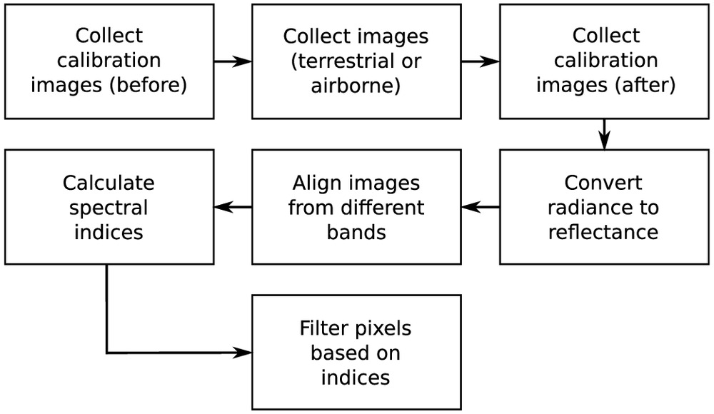
The methodology for image collection and processing is illustrated in Fig. 1. The image collection process, as shown on the first row, is discussed in the “Data Collection” section. The steps for transforming raw radiometric images into calibrated reflectance images, as shown on the second and third rows, is discussed in the “Data Processing” section.

Data Collection

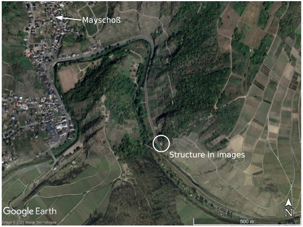
A team from GEER was deployed to western Europe to gather perishable data and document the impacts of the flood in August 2021 (Stark et al. 2021). The team explored the use of ground-based multispectral imagery with the objective to apply this technology in postdisaster data collection and reconnaissance efforts. In total, 112 images were collected, of which seven images contained the flooded building used to extract the high-water mark. The multispectral imagery collection was limited to a section of the Ahr River south of Mayschoss (Fig. 2).

Multispectral images were collected using a MicaSense Altum camera (Seattle), which simultaneously takes images in the blue (443 to 507 nm), green (533 to 587 nm), red (654 to 682 nm), red-edge (705 to 729 nm), near-infrared (785 to 899 nm), and thermal or long-wave infrared (5 to 17 μm) bands. Normally, this type of camera is deployed using UAVs and is mounted such that primarily nadir images are captured. However, in the case of postdisaster reconnaissance, certain features of interest, such as building walls or trees, for example, may not be adequately captured through purely nadir imagery. Thus, as part of this exploratory application, multispectral images were collected by carrying the camera by hand. The hand-held utilization was enabled by powering the camera externally using battery packs and manually triggering image collection through a cellphone connected to the camera’s Wi-Fi network.

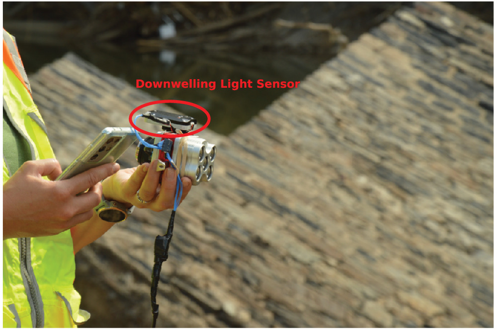
Additionally, as shown in Fig. 3, the downwelling light sensor (DLS) was connected to the camera to ensure it moved with the camera when images were taken. Although the setup shown in Fig. 3 ensured that the global positioning system (GPS) location for the images was correct, the orientation of the DLS for measuring incident light was off by 90°, and thus did not provide accurate measurements of sun-to-sensor angle and the direct and diffuse irradiance components. As such, the DLS measurements were not used for time-varying calibration, which instead relied on calibrated reflectance panel images taken at the beginning and end of date collection to convert radiance images to reflectance.

Fig. 3. MicaSense Altum with downwelling light sensor (DLS) connected directly to camera. The DLS is the flat plastic piece connected to the wire above the camera, as indicated on the image. A cellphone used to manually trigger camera through Altum Wi-Fi. (Image by Michael Gardner.)

Data Processing

Radiometric Calibration

The digital number pixel values from the multispectral imagery must be converted to reflectance values in order to calculate spectral indices. As mentioned in the “Data Collection” section, this conversion is determined based on images of a calibrated reflectance panel taken at the beginning and end of data collection. The processing discussed below was performed manually using functionality provided by MicaSense (2023) in their image processing GitHub repository.

The first step in this process was converting the raw pixel values to absolute spectral radiance,

L

, which for the MicaSense sensors was done as follows (MicaSense 2022):

L = V (x, y) \cdot \frac{a_{1}}{g} \cdot \frac{p - p_{BL}}{t_{e} - a_{2} y - a_{3} t_{e} y}

(1)

where

p

= normalized digital number pixel value;

p_{BL}

= normalized black level value;

a_{1}

,

a_{2}

, and

a_{3}

= radiometric calibration coefficients;

V (x, y)

= vignette polynomial function for a pixel located at

(x, y)

;

t_{e}

= image exposure time; and

g

= sensor gain setting. The parameters and settings in Eq. (1) were read from the image metadata. MicaSense sensors use a radial vignette model, defined as follows:

V (x, y) = \frac{1}{k}

(2)

where

k = 1 + k_{0} r + k_{1} r^{2} + k_{2} r^{3} + k_{3} r^{4} + k_{4} r^{5} + k_{5} r^{6}

(3)

r = \sqrt{{(x - c_{x})}^{2} + {(y - c_{y})}^{2}}

(4)

where

c_{x}

,

c_{y}

, and the polynomial coefficients

k_{1}

through

k_{6}

were read from the image metadata. Once the digital number pixel values have been converted to radiance, a transfer function for each of the sampled bands is calculated based on the average radiance of pixels on the calibrated panel area (MicaSense 2022)

F_{i} = \frac{ρ_{i}}{{\bar{L}}_{i}}

(5)

where

F_{i}

= radiance-to-reflectance factor for band

i

;

ρ_{i}

= reflectance value for the calibrated panel for band

i

; and

{\bar{L}}_{i}

= mean radiance of pixels on the calibrated panel area. The panel image was taken to match the orientation of the camera during image collection—normally the panel is placed flat on the ground because nadir images are collected from UAVs, but in this case images were collected with the camera orientation approximately parallel to the ground.

Spectral Index Calculation

Once the images have been radiometrically corrected, the images from different bandwidths must be aligned in order to generate pixel-accurate spectral indices or composite images. During the alignment process, an affine transformation is found to align each of the band images to a common band (the green band in our analyses). Once a transformation is found, the images are aligned and pixels that do not overlap are removed. Fig. 4 shows a true-color composite image created by combining the red, blue, and green band images, and Fig. 5 shows the set of reflectance images from which this true-color image was created.

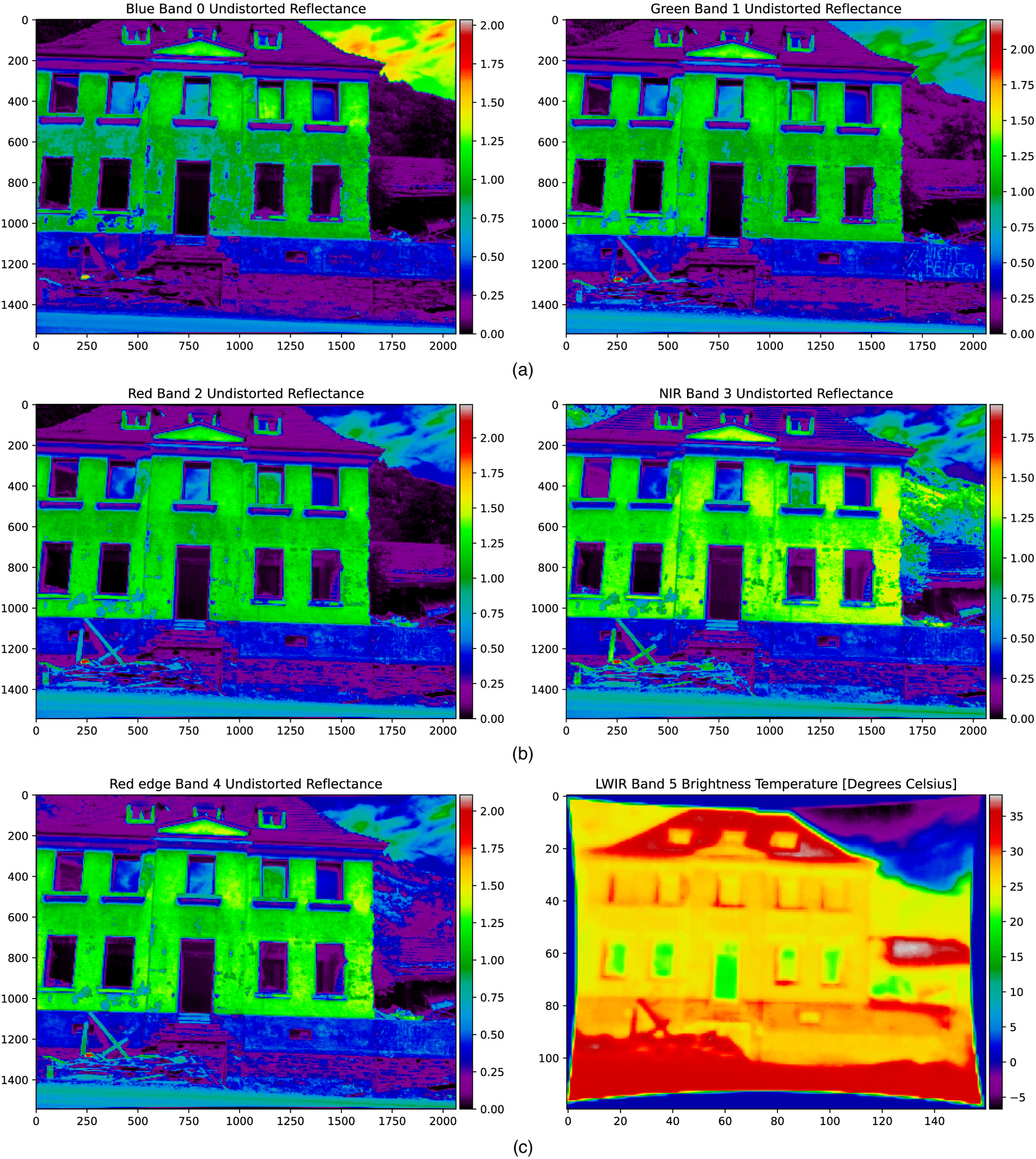
Fig. 4. True-color composite image created by combining the red, blue, and green band images. Here, the high-water mark was measured in the field, as indicated by the horizontal line. (Images by authors.)

Fig. 5. (a–c) Calibrated reflectance images of western face of the building where $x$ - and $y$ -scales indicate pixel locations. A clear manifestation of the high-water level in the blue band is shown in plot (a). (Images by authors.)

The high-water mark from flooding is still visible to the trained eye in the red-green-blue (RGB) composite image (Fig. 4), but it manifests clearly in the blue band, where there is a visible difference in the reflectance for plaster portions of the structure that were above and below the physically mapped high-water mark. This signal also appears in the green and red bands, but not as strongly as in the blue band. Comparatively, the near-infrared and red edge bands show evidence of the high-water mark, but the signal is not as clear or consistent throughout the region of the building facade that was below the flood level. The high-water mark in the different bands is likely associated with increased adsorption with increased moisture content. This concept was illustrated by Conde et al. (2016), where the relative change in adsorption of concrete as a function of moisture content was shown to differ across wavelengths and shown to be more prominent in the blue and green bands compared with red and red-edge bands. This matches our observation where the blue band was displaying regions of the building facade below the high-water mark (which can be assumed to have a higher residual moisture despite the time passed since the event) most clearly. The exact composition of the building facade is unknown, but appears to be a painted plaster-material.

Based on the initial manifestation of the high-water mark in the blue band, we explored combining different spectral bands to help isolate the signal associated with the water level on the building facade. Given that the high-water mark can be seen with varying levels of confidence across all bands, there likely are material-specific reflectance characteristics that modify reflectance in different bands. Additionally, as can be seen in Fig. 4, the coloration of the building was modified due to soil particles that adhered to the facade after flood levels subsided, which may also be contributing to the varying reflectance in different bands. Based on these observations, we calculated the difference between the red-edge and blue bands on a pixel-by-pixel basis. This combination of the blue and red-edge bands is designed to amplify the sections of the building facade that have increased adsorption in the blue band due to material-specific changes as a function of moisture content, as well as the increased adsorption in the red-edge band due to higher moisture content.

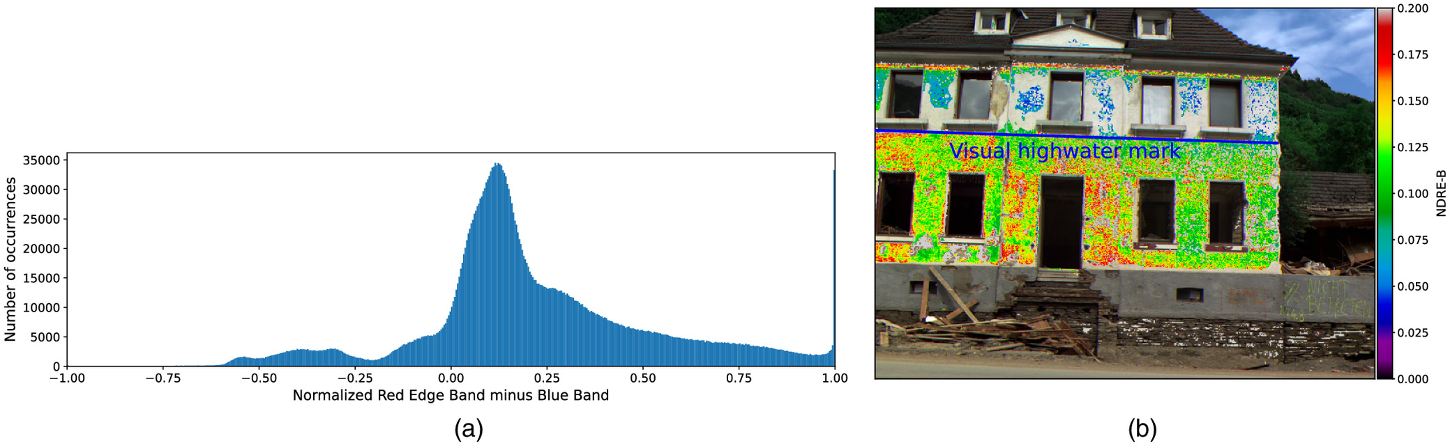
By subtracting the blue band from the red-edge band, which have similar reflectance values above the high-water mark, the resulting index value will be smaller. For regions below the high-water level, the difference in reflectance values is increased which yields a larger index value. Thus, higher values for the difference between red-edge and blue bands potentially indicate material that is below the high-water mark. Fig. 6 shows the histogram of pixel values for the difference between the red-edge and blue bands, in which three modes can be distinctly separated. Mode 1 is associated with pixels that contain portions of the sky [Fig. 7(a)], whereas Mode 2 is associated primarily with concrete on the structure and reflections in windows [Fig. 7(b)]. When visualizing the pixels associated with Mode 3 [Fig. 7(c)], the portions of the building facade that are below the high-water mark can be distinguished based on the difference between the red-edge and blue bands.

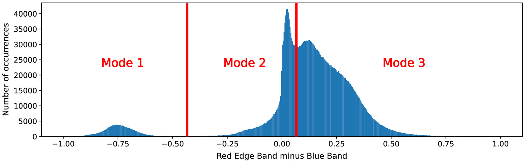
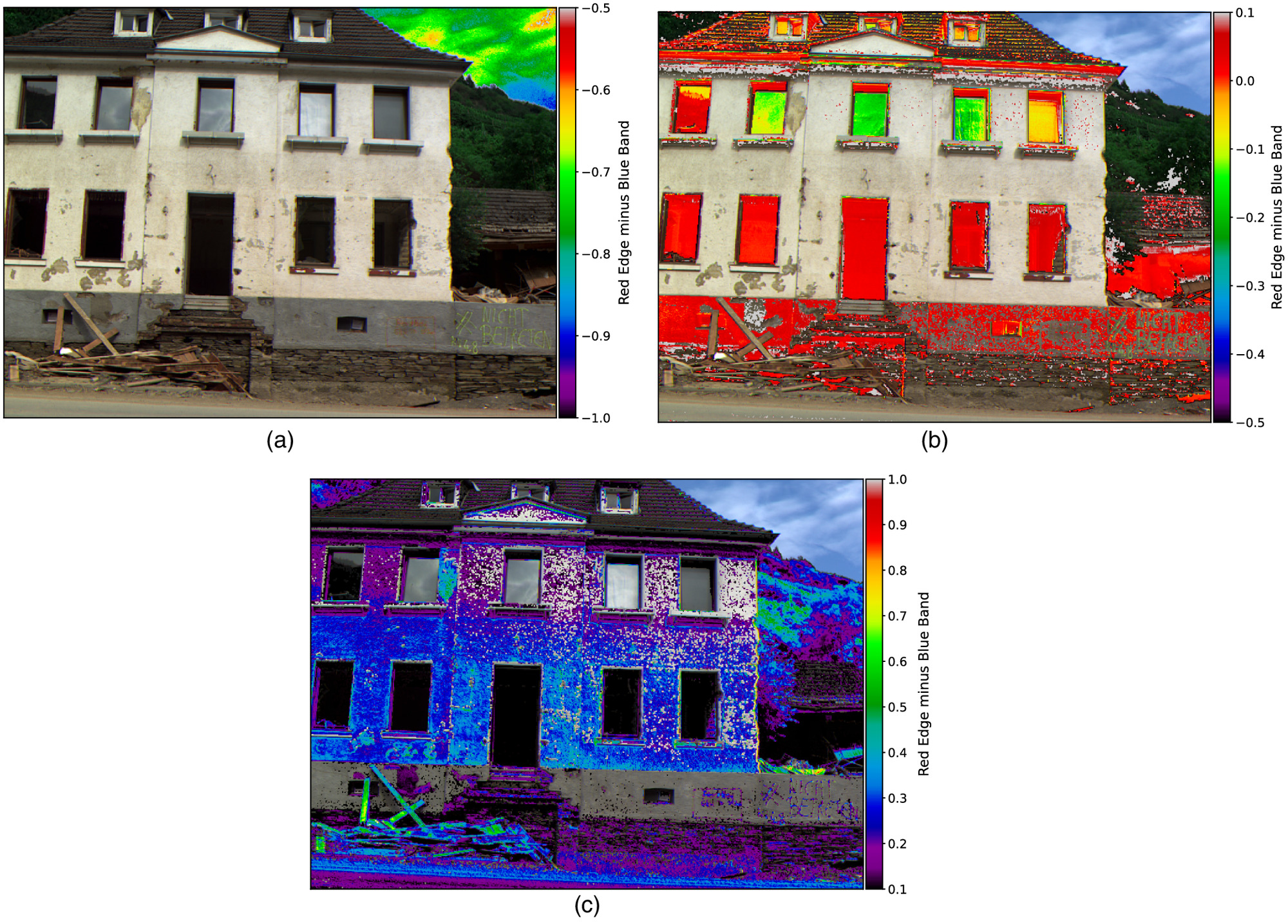
Fig. 6. Histogram on pixel-by-pixel basis of red-edge band minus blue band. Mode 1 is associated with pixels that contain portions of the sky, Mode 2 is associated primarily with concrete on the structure and reflections in the windows, and Mode 3 is excited by portions of the building facade.

Fig. 7. Pixels associated with modes in Fig. 6: (a) Mode 1; (b) Mode 2; and (c) Mode 3. The contrast in index values can be seen for pixels above and below the high-water mark for Mode 3. (Images by authors.)

Fig. 7(c) shows a strong signal that appears to be associated with the flood level. Noise was removed from this image due to pixels that were either not part of the building or a distinctly different material that may have different reflectance characteristics than the building facade. To remove any plants from the index calculation, we masked pixels for which the Normalized Difference Vegetation Index (NDVI) (Tucker 1979) was greater than 0.2. This is based on observations that the NDVI for plants ranges from 0.2 to 1.0. Fig. 8(a) shows all pixels that have an NDVI of 0.2 or greater; these are the pixels that were masked to remove noise associated with pixels that contain plants.

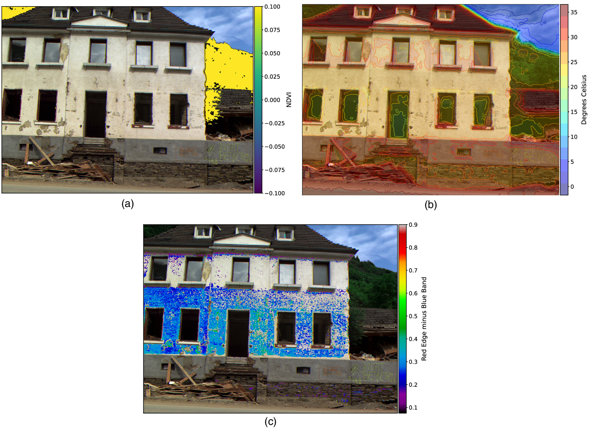
Fig. 8. Filtering to remove pixels associated with plants and building materials different from those in the building facade: (a) pixels with NDVI greater or equal to 0.2; (b) thermal contours (°C); and (c) Mode 3 pixels with masking applied for pixels with NDVI greater or equal to 0.2 and temperature greater than 27°C. (Images by authors.)

To further remove noise due to soil pixels and building materials different from the plaster in the facade, we used patterns from the thermal images that were collected simultaneously with the other multispectral bands. Contours of the temperature are overlain on the true-color composite to illustrate the heat signature across the entire image [Fig. 8(b)]. Because the thermal images are a lower resolution compared with the other spectral bands, a Lanczos interpolation over a

8 \times 8 pixel

neighborhood was applied when overlaying the thermal imagery on the multispectral images. The temperature across a building facade is generally lower in areas below the flood level, but significantly warmer areas on the same material can be identified above the flood level. Other building materials, such as concrete and roofing, also have substantially higher temperatures than the plaster on the building exterior. We suspect this difference in temperature is also at least partially due to moisture content within the building facade, as has been noted by others (Avdelidis et al. 2003; Moropoulou et al. 2018). Based on these observations, we further masked pixels where the temperature was higher than 27°C, as shown in Fig. 8(c), which almost entirely isolates the pixels that were below the high-water level and effectively depicts the high-water mark. The selected temperature threshold will be influenced by the time of day the pictures are taken because temperature differences potentially would be higher due to varied material heating rates during warmer parts of the day.

In order to isolate the high-water mark into a single mode that can be identified automatically, we further explored normalizing the difference between the red-edge and blue bands, denoted as NDRE-B for brevity:

NDRE - B = \frac{Red - Edge - Blue}{Red - Edge + Blue}

(6)

where Red-Edge = calibrated reflectance in the red-edge band; and Blue = calibrated reflectance in the blue band. Fig. 9(a) shows the histogram of calculated pixel values for this normalized index, where a single mode can be seen ranging from approximately 0.0 to 0.2. Applying the same NDVI and temperature filters as were applied to the Mode 3 plots [Fig. 8(c)], NDRE-B is shown in Fig. 9(b). The high-water mark can also be clearly seen in this image, although it is important to note the high values of the index in the shaded regions just below the roof of the structure.

Fig. 9. Normalized difference between red-edge and blue bands (NDRE-B): (a) histogram of NDRE-B pixel values showing single mode ranging from approximately 0.0 to 0.2; and (b) pixels with NDRE-B ranging from 0.0 to 0.2. Shady areas immediately beneath roof also yielded a high value for this index. (Images by authors.)

Discussion

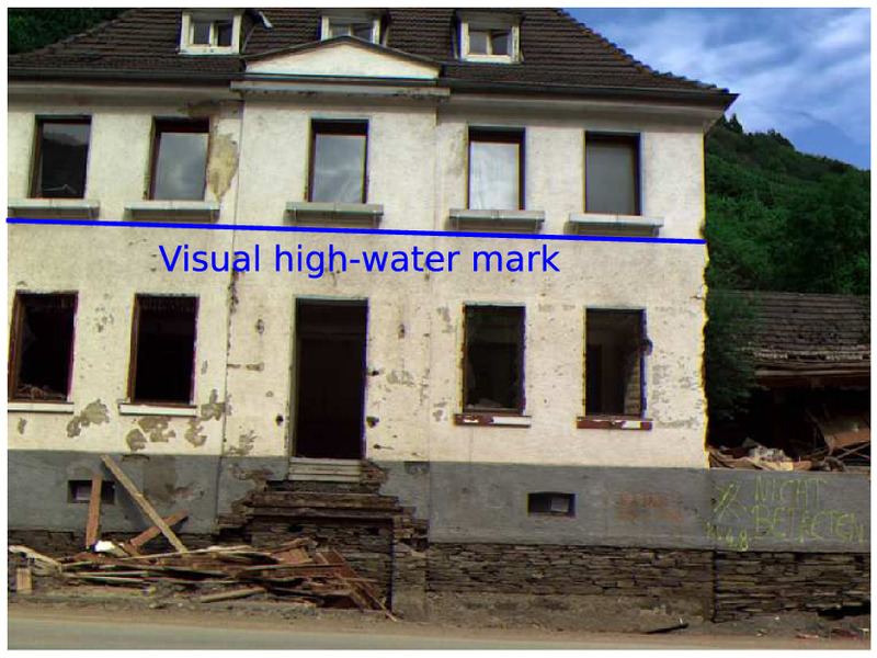
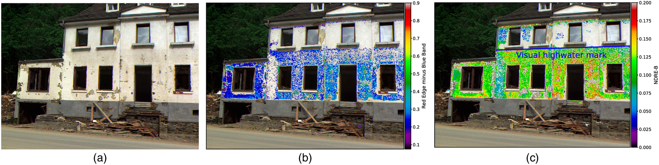
The initial results presented here promise potential for using multispectral imagery for postflood high-water mark display and mapping. This is illustrated in Figs. 9 and 10, which show the high-water mark estimated from the mulstispectral imagery using the proposed index calculation. Specifically, Figs. 9(b) and 10(c) show very good matching between the high-water mark estimated from the multispectral imagery and the physically observed value. The estimated values were within centimeters of those observed by the GEER team during the reconnaissance mission and are consistent across the entire facade of the flooded building. High-water marks represent key information to document the extent and severity of flooding. In this case, multispectral images were taken by a surveyor carrying the camera when safe access to the disaster area was possible. Future deployments could also utilize UAVs to collect images of structures and infrastructure in areas that may not be accessible on foot in order to broadly map high-water levels spatially.

Fig. 10. Potential influence of sediment adhering to building facade: (a) true-color composite showing less discoloration and sediment adhesion to building at the single- and two-story interface; (b) weaker high-water signal in region near single- and two-story interface based on difference between red-edge and blue bands; and (c) NDRE-B showing similar weaker signal near single- and two-story interface. (Images by authors.)

To apply the technique presented in this paper more broadly, additional research is underway to establish the suitability of this approach for different building materials. As visible in Fig. 7, the concrete material located at the bottom of the building did not bin to the Mode 3 region (Fig. 6) like the plaster material, even though both materials were clearly below the high-water mark. This can also be seen in portions of these images where the plaster has been damaged and removed, yielding different reflectance values compared with immediately adjacent material. Thus, reflectance characteristics for commonly used building facade materials need to be established, particularly to develop an automated high-water mark detection procedure.

Images with a broader range of spectral bands may also improve confidence in the high-water mark identification because the five bands sampled in this case study may not be sufficient for all types of material used in building facades. Furthermore, high-water marks apply naturally over large areas under a certain elevation; thus, the application of an averaging or stochastic data analysis procedure, as well as edge-detection algorithms, should be explored because it is unlikely that the current approach is prepared for any materials encountered in postflood reconnaissance. This will help eliminate false high-water marks [as seen immediately beneath the roof in Fig. 10(c)] where the index values of several pixels would indicate that the high-water extended to this elevation; however, neighboring index values indicate that pixels at lower elevations do not support labeling this elevation as the high-water mark. This work is ongoing and outside the scope of this article.

The manifestation of the high-water mark in the multispectral imagery is typically linked to the moisture content or soil and other material particles stuck to the original structure or object. Moisture content can be subject to change with time from environmental conditions such as solar radiation or new rainfall. Similarly, particle traces can be washed away by new rainfall or by active cleaning efforts. In this study, it was assumed that the high-water mark is mostly representing a change in moisture content, despite an extended period of high air temperatures and solar radiation after the flood and before the data collection. This assumption was based on the decreasing signal strength across the portion of the building facade, as seen in Figs. 7(c) and 8(c), when approaching southern directed faces of the structure. These portions of the building receive sunlight more directly and for longer hours, so likely were drier than other portions of the building at the time of image collection. Flooding occurred from July 14 to 15, 2021, and the image collection only occurred on August 11, 2021 (i.e., almost 1 month after flooding). We suspect the image signal to be more uniform closer to the time of flooding; however, that the flooding level can still be clearly seen in the multispectral images several weeks after flooding occurred represents a key finding because it promises higher reliability in high-water mark detection in situations where immediate access for postdisaster surveyors is difficult and measurements cannot be taken until days or weeks after the event.

Lastly, the reflectance characteristics of the building materials will be influenced by the amount and type of sediment transported during flooding and how it adheres to building surfaces after flooding has subsided. Based on the authors’ preliminary analyses, it was not immediately evident how much sediment adherence may contribute to the signal in the multispectral imagery; however, it is likely an effect that cannot be ignored. This is illustrated in Fig. 10, where the true color composite and the difference between the red-edge and blue bands are shown side by side. The lighter-colored region near the interface between the single- and two-story portions of the structure does not show the below-flood level as clearly as other regions of the building facade [Fig. 10(b)]. However, this is not the case for the lower signal strength in the lower right portions of the building facade shown in Fig. 8(c), where the discoloration is uniform, indicating the decrease in signal is associated with a different characteristic—potentially moisture content, as discussed previously.

Conclusion

In order to better meet the challenges posed by the evolving hazard associated with extreme flooding, it is necessary to be able to quickly and effectively map the extent of flooding and the damage caused by it. One of the key pieces of information desired in flood reconnaissance data collection is high-water marks. However, high-water marks can change with time postflood due to environmental conditions and active repair and cleanup efforts, and postflood surveyors can often not safely access the disaster immediately after the event. Thus, there is a need for increasing the detection, and reliability in detection, of high-water marks days to weeks after the flood event.

This case study suggests a great potential for using multispectral images to map high-water marks on buildings affected by flooding, in this case, approximately 4 weeks after the event and after significant exposure to heat, solar radiation, and local cleanup efforts. This application of multispectral imagery for high-water mark detection will allow for rapid and broad mapping of spatially varying high water. This will enable more accurate assessment of the flood extent and depth, as well as a means to determine potential volumes of waste that may be generated during recovery and reconstruction efforts.

The high-water mark clearly manifested in the blue band through increased adsorption in portions of the building that were below the high-water level and likely featured higher moisture content in the building facade material. The high-water mark was modally isolated through a linear combination of the blue and red-edge bands. This linear combination amplified the increased adsorption in both the blue and red-edge bands. By differencing these two bands, regions with higher reflectance (lower adsorption due to lower moisture content) canceled out, whereas regions with lower reflectance (higher adsorption due to higher moisture content) were amplified due to the large differences in adsorption characteristics between the blue and red-edge bands for the building material investigated.

Initial data collection was limited and presented results for only one type of building facade material. Different building materials will likely have varying spectral signatures, and it may be necessary to establish which bands should be sampled or to explore stochastic data analysis procedures and change detection to ensure that flooding characteristics can be broadly mapped using multispectral imagery. Careful consideration of temperature variations due to material heating rates, intensity, and length of time buildings are exposed to solar radiance, time of day images were collected, and potential interaction with sediment adhering to the building facade should be included in future research. Future applications may also consider the combined use of ground-based and UAV-based image collection.

Data Availability Statement

Some or all data, models, or code generated or used during the study are available in a repository or online in accordance with funder data retention policies. All data collected during the GEER reconnaissance can be found at this link (https://doi.org/10.17603/ds2-0ddt-ss87). All the functionality provided by MicaSense can be found in the GitHub repository at this link (https://github.com/micasense/imageprocessing).

Acknowledgments

This research was supported by the National Science Foundation (NSF) through the Geotechnical Extreme Event Reconnaissance (GEER) Association, under Award No. CMMI-1826118, and awards CMMI-2213768, -2213715, -2213714. Data was collected in part using instrumentation provided by the NSF as part of the RAPID Facility, a component of the Natural Hazards Engineering Research Infrastructure, under Award No. CMMI-2130997. Any opinions, findings, conclusions, and recommendations presented in this paper are those of the authors and do not necessarily reflect the views of NSF.

References

AON. 2021. “Global catastrophe recap July 2021.” Accessed July 17, 2022. http://thoughtleadership.aon.com/Documents/20211008_analytics-if-july-global-recap.pdf.

Abstract

Introduction

Data Collection and Processing

Data Collection

Data Processing

Radiometric Calibration

Spectral Index Calculation

Discussion

Conclusion

Data Availability Statement

Acknowledgments

References

Information

Published In

Copyright

History

ASCE Technical Topics:

Authors

Affiliations

Metrics

Citations

Download citation

Cited by

Figures

Other

Share

Copy the content Link

Share with email

Share

Request Username

Create a new account

Change Password

Password Changed Successfully

Verify Phone

Congrats!