Hazus Hurricane Wind Model for the US Caribbean Territories: Hazard Modeling and Development of Residential Damage Functions
Abstract
The Hazus Hurricane Model has been extended to include the US Virgin Islands and Puerto Rico. The hurricane hazard model uses the same model incorporated into the design wind speeds given in US and Caribbean wind loading provisions wind hazard maps for the US mainland and the US Caribbean islands. The validity of the hurricane hazard model for use in the Caribbean is documented herein. New damage functions were developed to model the different construction methods used in the region as compared to the mainland United States. These damage functions include new models for metal roofs developed using finite-element analyses and then parameterized for use with a range of sizes, metal thicknesses, and attachment spacings.
Introduction
The extension of the Hazus Hurricane Model to include the US Caribbean territories required the development of hurricane wind hazard data as well as the development of new damage functions to better model the types of construction found in the US Virgin Islands (USVI) and Puerto Rico (PR). The hurricane hazard data for PR and the USVI were created using the version of the Hurricane Model used to develop the wind hazard data given in ASCE 7-22 (ASCE 2022).
The new damage functions introduce the capability to model buildings with various metal roofs common in both the USVI and PR, plywood roofs with liquid applied waterproof membranes common in the USVI, and informal construction (completed outside of the normal design and permitting process) found in PR. The new damage functions apply only to single-family residential construction and incorporate updates to both the wind load models and the loss given damage models.
Hurricane Model Updates
The hurricane simulation approach used to define the hurricane hazard in PR and the USVI comprises two major components. The first component comprises a hurricane track model that reproduces the temporal and spatial characteristics of hurricane tracks as well as the variation of hurricane size and intensity as hurricanes move along the tracks. The second portion of the model is the hurricane wind field model, which provides estimates of the wind speed and wind direction at an arbitrary location given key hurricane parameters, provided by the track model, at that location. The following sections describe the verification of the track model near PR and the USVI.
Hurricane Track Modeling
The hurricane track and intensity simulation methodology used to define the hurricane hazard in PR and the USVI follows that described in Vickery et al. (2000), Vickery and Wadhera (2008), but the coefficients used in the statistical models were calibrated to model the variation in storm characteristics throughout the Atlantic Basin.
The hurricane position at any point in time is modeled using the approach given in Vickery et al. (2000). Given the initial storm heading, translation speed, and intensity, the model estimates the new position and speed of the storm based on changes in the translation speed and storm heading over the current 6-h period. The changes in the translation speed and the storm heading between time steps and are obtained from Eqs. (1) and (2)where and = constants; , = storm latitude and longitude at time step i, respectively; = storm translation speed at time step ; , = storm heading at time step and , respectively; and = random error term. The coefficients were developed using grids over the Atlantic Basin. A different set of coefficients for easterly and westerly headed storms is used.
(1)
(2)
The relative intensity, , of the hurricane is modeled using a modified version of the approach given in Vickery et al. (2000) as described in Vickery et al. (2009b). The relative intensity is then used to compute the central pressure, as described in Vickery et al. (2000). Then, using this central pressure, the radius to maximum winds (RMW) and the Holland (1980) parameter are computed as described in Vickery and Wadhera (2008). A simple one-dimensional ocean mixing model, described in Emanuel et al. (2006), is used to simulate the effect of ocean feedback on the relative intensity calculations. The ocean mixing model returns an estimate of a mixed layer depth that is used to compute the reduction in sea surface temperature caused by the passage of a hurricane. This reduced sea surface temperature is used to convert historical pressures to relative intensity values. The historical relative intensity values are then used to develop regional statistical models in the form of Eq. (3), where the relative intensity at each new time step is modeled as a function of relative intensity at the preceding three time steps and the scaled vertical wind shear, , at the preceding time step (DeMaria and Kaplan 1999)where = constants that vary with region in the Atlantic Basin; = environmental wind shear; and = random error term. If a storm crosses land, the central pressure is computed using a filling model, where the central pressure hours after landfall is dependent on the storm pressure at the time of landfall and the number of hours the storm has been over land.
(3)
Storm Filling
As in Vickery (2005), weakening of the hurricane after landfall was modeled using an exponential decay (filling) function in the form of Eq. (4)where = central pressure difference hours after landfall; = central pressure difference at the time of landfall; and = empirically derived filling coefficient. If not specified explicitly in HURDAT2, the landfall pressure was computed from the HURDAT2 database by extrapolating the central pressures using the last two central pressures before landfall. Using this approach, the pressure tendency of the hurricane before landfall is maintained, such that weakening storms continue to weaken and strengthening storms continue to strengthen until landfall.
(4)
For PR, is modeled as in Eq. (5), where RMW is the radius to maximum winds
(5)
In the case of the USVI, storms were not filled even if they crossed one of the islands. Any storm weakening that may occur due to interactions of the storm center with one of the USVI is handled only to the extent that such weakening appears in the historical records.
Hurricane Track and Intensity Model Validation
The HURDAT2 data set used in the model validation includes all tropical cyclones during the period 1900 through 2018. However, central pressure data are only available for about 37% of the data points in the Caribbean. As in Georgiou et al. (1983), Georgiou (1985), and Vickery and Twisdale (1995), we assume that the missing central pressure data belong to a population having the same statistical distribution (given the occurrence of a storm) as that computed using the nonmissing data.
In the model validation process, we compared the statistics of storm heading, translation speed, central pressure, and annual occurrence rates for modeled and historical storms passing within 250 km of grid points spaced at 2° intervals from 16° to 20° N and 62° to 68° W. The heading and translation speed are computed at the point of closest approach to the center of each circle. The central pressure values used in the validation procedure are the minimum values measured or modeled at any time while the storm is in the circle. Figs. 1 and 2 present comparisons of the modeled and historical cumulative distribution functions (CDFs) of storm heading and translation speed near PR and the USVI. Fig. 3 presents comparisons of modeled and observed central pressures plotted versus return period near PR and the USVI.
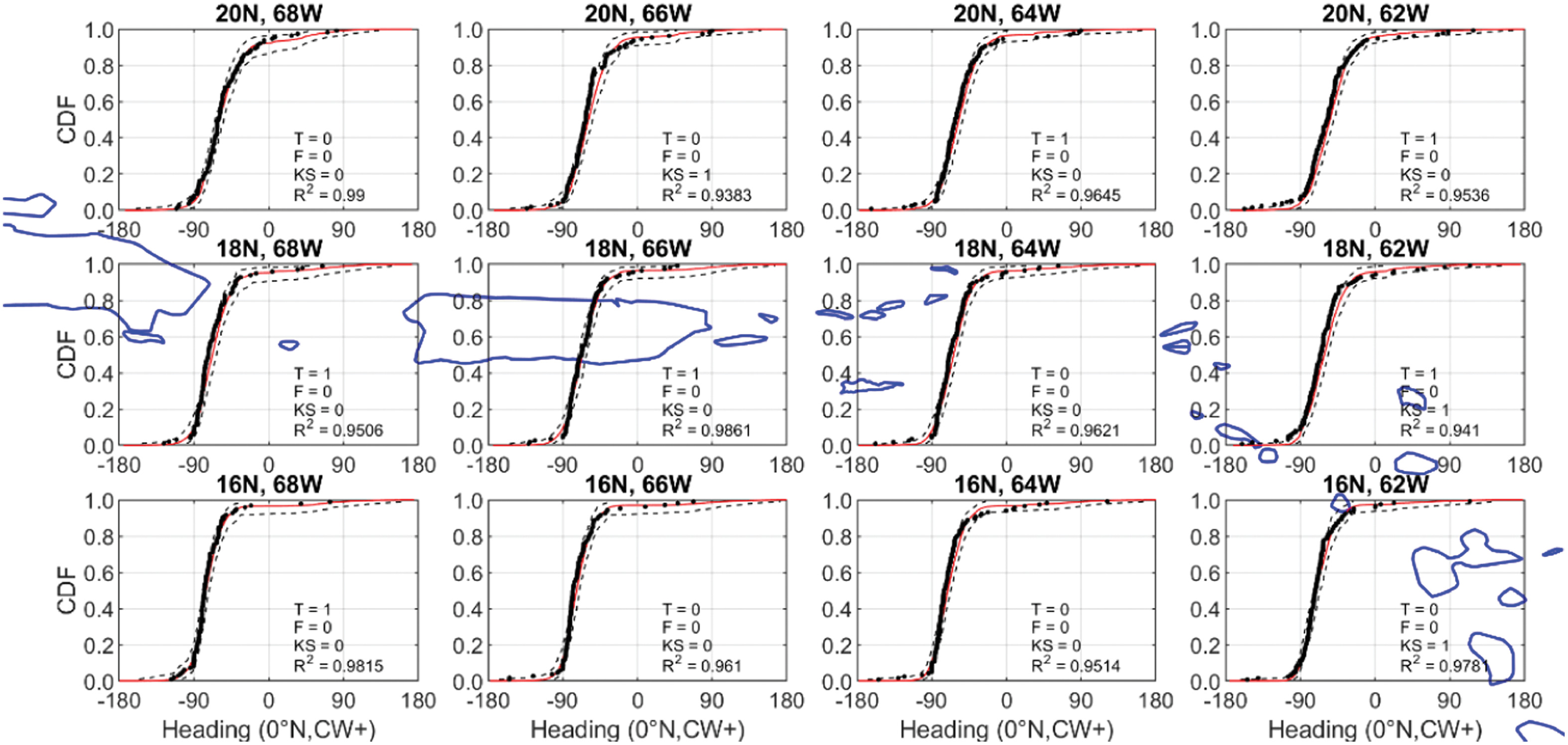
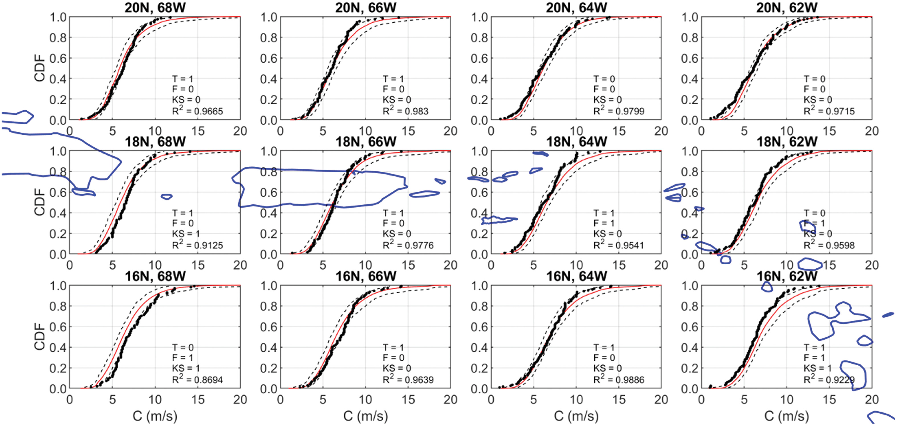
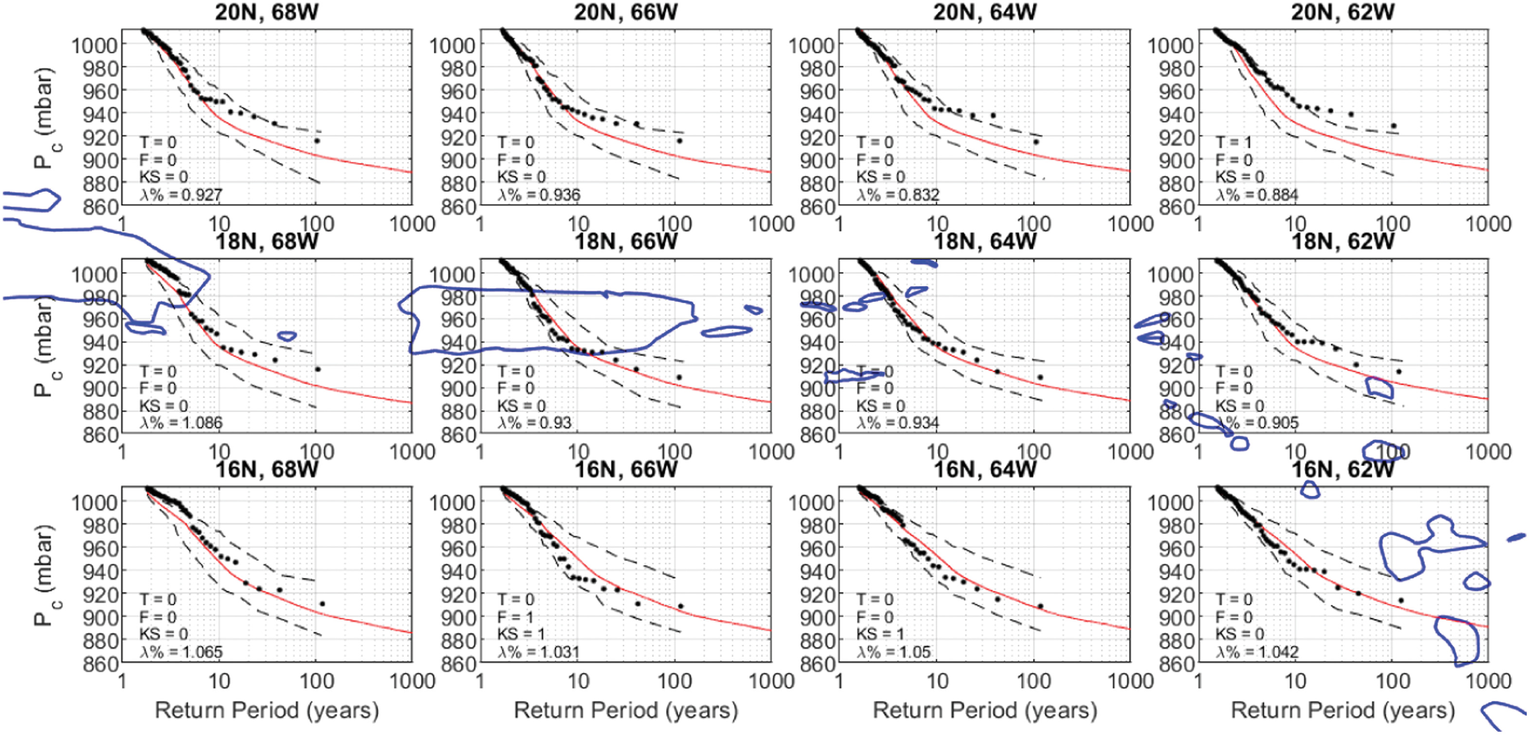
To verify the ability of the model to reproduce the characteristics of historical storms, we also performed statistical tests comparing the characteristics of modeled and observed hurricane parameters. The statistical tests include the -test for equivalence of means, the -test for equivalence of variance, and the Kolmogorov-Smirnov (K-S) test for equivalence of the CDF. The equivalence testing of the pressure-return period curves yields a comparison that includes the combined effects of the modeling of both the central pressures and the frequency of occurrence of the storms. In Figs. 1–3, a value of 1 next to the indicated test implies failure at the 95% confidence level. No consideration is given to the measurement errors inherent in the HURDAT2 data in any of the statistical testing.
Hurricane Wind Field Modeling
The hurricane wind field model used in Hazus is described in detail in Vickery et al. (2009a), and only a brief summary is presented here. The model solves the Navier-Stokes equations for a two-dimensional (2D) slab of a translating hurricane driven by a known pressure field over a surface with surface friction, modeled as either marine or open terrain. The pressure field used is described in Holland (1980) and is characterized using three terms, namely, the RMW, the Holland (1980) shape-intensity parameter, , and the central pressure deficit, . The surface friction produces asymmetries and inflow much different than those associated with wind field models that do not consider surface friction. The equations of motion are solved using a nested grid with the smallest grid size equal to 10% of the radius to maximum winds. The 2D slab model is converted to a simple three-dimensional (3D) model using a boundary layer model describing the variation of the mean wind speed with height. The boundary layer height used in the boundary layer model varies over the domain of the storm, reaching a minimum near the RMW. The mean surface-level wind speeds are converted to gust wind speeds using the ESDU (1982, 1983) models for atmospheric turbulence. The hurricane wind field model has been extensively validated through comparisons between modeled and measured surface level mean and gust wind speeds, and surface pressures.
Wind Hazard Results
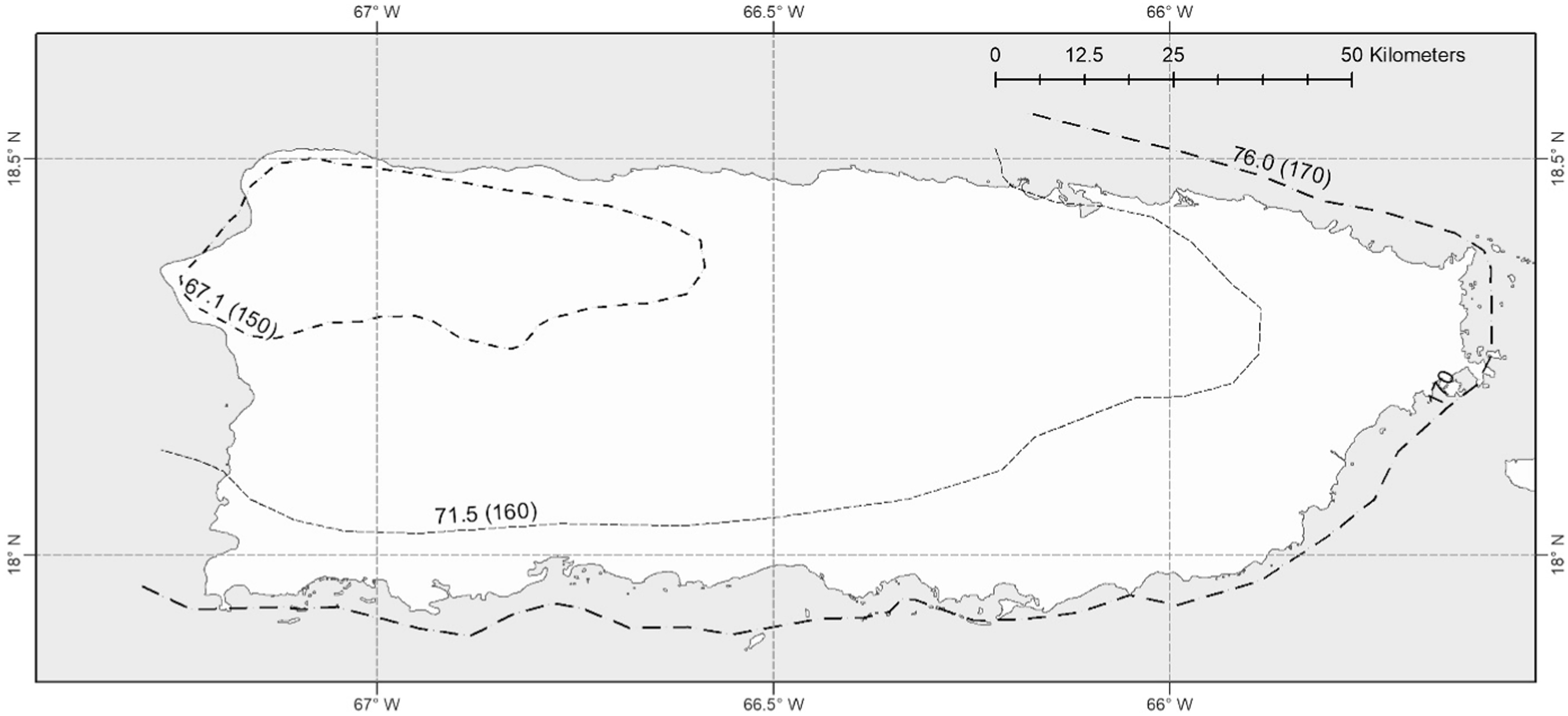
The 700-year return period wind speeds resulting from the 100,000-year hurricane simulation are shown in Fig. 4 for Puerto Rico. In the damage and loss estimation in Hazus, the wind speeds resulting from the hurricane simulation are combined with the topographic speed-up model described in Vickery et al. (forthcoming) to account for the effects of the complex topography in Puerto Rico and the USVI. The topographic speed-up model is the same as that used to develop the wind speeds, including the effects of topography, given in ASCE 7-22.
Development of Damage and Loss Functions
The unique characteristics of the residential building stock in the USVI and PR could not be modeled using the existing Hazus damage functions, which were developed for use in the contiguous United States and Hawaii. Examples of building stock characteristics present in the USVI and PR that differ from the damage functions currently in Hazus include:
•
Informal construction in PR typically comprising a masonry lower story with a wood-frame second story, and a corrugated metal roof nailed to wood rafters with spacing of 1.22 m (4 ft).
•
The prevalence of jalousie windows.
•
Single-family residences with concrete roofs.
•
Single-family residences with standing seam metal roofs mounted on a plywood or oriented strand board (OSB) roof deck.
•
Single-family residences with an elastomeric waterproof coating over a plywood or OSB roof deck.
To model the building types and their characteristics typical in PR and the USVI, new damage curves had to be developed to include corrugated metal roof panels, standing seam metal roof panels, and jalousie windows. The failure pressures were computed using finite-element models. The capacity of the jalousie windows was obtained through a literature search of experimental studies examining the pressure resistance of jalousie windows. Additional building characteristics unique to the regions such as differences in wall construction between the islands and the mainland United States and the use of post-and-beam construction in masonry buildings were not modeled.
Development of Fragilities for Metal Roof Panels
The version of Hazus developed for the contiguous United States does not have the capability to model metal roofs on single-family homes. Because metal roofs are common in both PR and the USVI, it was necessary to add the ability to model them. Three types of metal roofs were considered, namely:
•
Corrugated metal nailed or screwed to wood battens, usually associated with informal construction.
•
Standing seam metal attached to metal purlins using clips.
•
Standing seam metal attached to plywood or OSB decking using screws.
In all cases, the metal roof serves as the water-resistant barrier. Because there is limited public domain information on the uplift capacities of metal roofing systems, finite-element analyses (FEA) were performed to develop the uplift capacities of the metal roof systems examined.
Corrugated Metal Roofs
Corrugated metal roofs are commonly used in informal construction where a second story comprising a wood-frame structure is added above an existing one-story masonry or concrete structure. The corrugated metal panels are usually nailed to battens, which may be spaced up to 1.22 m (4 ft) apart, resulting in a relatively weak roofing system. The analysis of the corrugated metal panel uplift capacity considered a range of metal panel thicknesses, purlin spacings, and two methods of attachment (nails and screws). Sensitivity studies varying the gauge (thickness) of the metal, fastener spacing, and batten spacings were performed.
The uplift capacities of the metal panels were all computed using FEA, specifically using the ANSYS software package. This same approach was used to develop the uplift resistances of the engineered metal deck currently used in Hazus for commercial buildings having metal decks fastened to open web steel joists using mechanical fasteners or welds (Vickery et al. 2006). The metal panels used in commercial structures are much different (thicker panels generally welded to open web steel joists) than the metal panels used for light-frame residential construction.
Detailed finite-element models of the corrugated metal roof were developed to evaluate the wind uplift capacity for metal panels connected to the supporting battens using 8d common nails. The finite-element models were developed using the techniques presented in Mahendran (1990, 1992, 1994). The metal panels were modeled using elastic orthotropic 3D shell elements defined by four nodes having six degrees of freedom at each node. The shell element has shear, bending, and membrane stiffness, and is also well suited for linear, large rotation, and large strain nonlinear applications. The battens and trusses are modeled using isotropic 3D beam elements. The connections between metal panels and the supporting battens are modeled using a nonlinear spring element that connects a pair of nodes with nonlinear generalized force–displacement capability. This spring element is unidirectional; hence each 8d nail connection is modeled with three independent nonlinear spring elements to account for one axial and two lateral stiffnesses representing load–displacement relationships in the -, -, and -directions. This type of element has been successfully used for numerical simulation of timber structures by Kumar et al. (2012) and Pan et al. (2013). The metal panel roof system was analyzed by applying uniform wind uplift pressure with boundary conditions applied only to the fastener locations.
The finite-element model accounts for the anisotropic and nonlinear material properties of the cladding as reported in the study by Lovisa et al. (2013) for a G550 corrugated metal sheet. The material properties of the G550 corrugated metal sheet, including the strain hardening characteristics, were incorporated into the numerical model through a multilinear kinematic hardening model developed by fitting an experimental stress–strain curve (Xu and Teng 1994; Lovisa et al. 2013). The isotropic elastic modulus and Poisson’s ratio for wood battens were obtained from Doudak (2005) and Martin et al. (2011), respectively. The force–displacement responses used in the modeling of nonlinear springs representing 8d nail connections were obtained from test results reported by Thampi (2010), where the connection was tested under withdrawal load, lateral slip, and moment to characterize the nail behavior.
The finite-element models of a corrugated metal roof with nail connections between metal claddings and battens could not be validated due to unavailability of experimental responses on such roof systems. However, the finite-element models were validated against experimental responses of a corrugated metal roof system where the metal claddings were connected to battens using sheet metal screws. These experimental data were taken from the studies of Xu and Reardon (1993) and Lovisa et al. (2013), where a 26-gauge corrugated metal roof having a 900-mm span was tested under static uplift loads. The finite-element models were developed according to the experimental setup and material properties specified in Xu and Reardon (1993) and Lovisa et al. (2013). The simulated uplift pressures versus vertical deflections of the metal panels are compared to the measured responses in Fig. 5, where it is seen that the finite-element models match the experimental uplift responses quite well.

Simulated von Mises stress contours of the corrugated metal roof system indicate that the stresses around the connections were close to the ultimate strength of sheet metal, suggesting a pull-through failure of the connection. This is consistent with the failure modes observed in the experiments by Xu and Reardon (1993), Lovisa et al. (2013), and more recently by Roy et al. (2018). Given that the numerical technique developed herein can accurately calculate the uplift resistance of a corrugated metal roof attached to battens using screws, the same model was used to investigate the uplift resistance of a corrugated metal roof with nail connections to battens.
The finite-element models were used to investigate the effect of batten spacing, panel width, nail spacing, and sheet metal gauge on the uplift resistance of a corrugated metal roof with nail connections to battens. In the analysis, the depth and the pitch distance of corrugations were taken as 16 and 76.2 mm, respectively. The nail spacing in the direction of the corrugation (-direction) was taken as 300 mm, while the nail spacing in the direction perpendicular to corrugation (-direction) was varied between 600 and 1,250 mm. The gauge of the metal was varied between 24 and 35 and the panel width and batten spacings were varied between 600 and 1,250 mm. The sensitivity to nail spacing was also examined. The governing failure mode of the corrugated metal roof where the metal claddings are connected to wood battens with nails was a pull-through failure of the sheet metal.
Uplift Resistance of Standing Seam Metal Roofs Connected to Roof Deck Using through Fasteners
Estimates of the uplift capacities of standing seam metal roofs connected to a plywood roof deck with sheet metal screws were also developed using FEA. The FEA was utilized to study the effect of seam height, metal thickness, fastener spacing, and panel width on the uplift capacity of the panels. Using the FEA results, parametric equations were developed to calculate wind uplift resistances of these standing seam metal roofs connected to plywood roof decks subjected to uniform uplift pressure.
The finite-element models were developed following the techniques presented in El Damatty et al. (2003). The material properties of the metal panels were taken from studies by Ali and Senseny (2003) and El Damatty et al. (2003). The force–displacement responses of the nonlinear springs representing the panel seams were obtained from test results reported by El Damatty et al. (2003) and El Damatty and Rahman (2004). The force–displacement responses for the nonlinear springs representing the fasteners between the metal panel and roof deck were obtained from the test results reported in Sivapathasundaram and Mahendran (2018). The finite-element models of the standing seam metal roof connected to the roof deck using through fasteners could not be validated due to unavailability of experimental responses of such roof system; however, the finite-element models of a standing seam metal roof connected to purlins using metal clips were validated against experimental responses, which are presented subsequently.
The uplift capacities of the standing seam metal roof were evaluated using a range of seam heights, metal panel thicknesses, fastener spacings, and panel widths so that the effect of each of these parameters could be investigated and a relationship developed to calculate static uplift resistances for arbitrary values of seam heights, panel widths, and so on.
Fig. 6 shows the uplift resistance for the base case example having a 610-mm-wide standing seam metal roof with 25.4-mm seam height plotted against the fastener spacing normalized by panel thickness (). It was found that the uplift resistance decreases nonlinearly with an increase in the ratio . Hence, the uplift resistance is expressed as a nonlinear function of the dimensionless quantity given aswhere = uplift resistance (kPa); = panel thickness (mm); and = fastener spacing (mm).
(6)

To calculate uplift resistances for different panel widths and seam heights, uplift resistances normalized to the base case (610-mm-wide standing seam metal roof with 25-mm seam height) were plotted against panel width and seam heights. The normalized uplift resistance was found to decrease nonlinearly with an increase in panel width and increase nonlinearly with an increase in seam height. By varying panel width and seam height in the FEA, factors were developed for an empirical model to be used for a range of panel widths and seam heights without the need of a new FEA. The factors and take into account the effect of panel width (mm) and seam height (mm), respectively, and are given aswhere = panel width (mm); and = seam height (mm). The uplift capacity of a standing seam metal roof panel for different panel thicknesses, seam heights, panel widths, and fastener spacing can be computed usingwhere = fastener spacing (mm); and = panel thickness (mm).
(7)
(8)
(9)
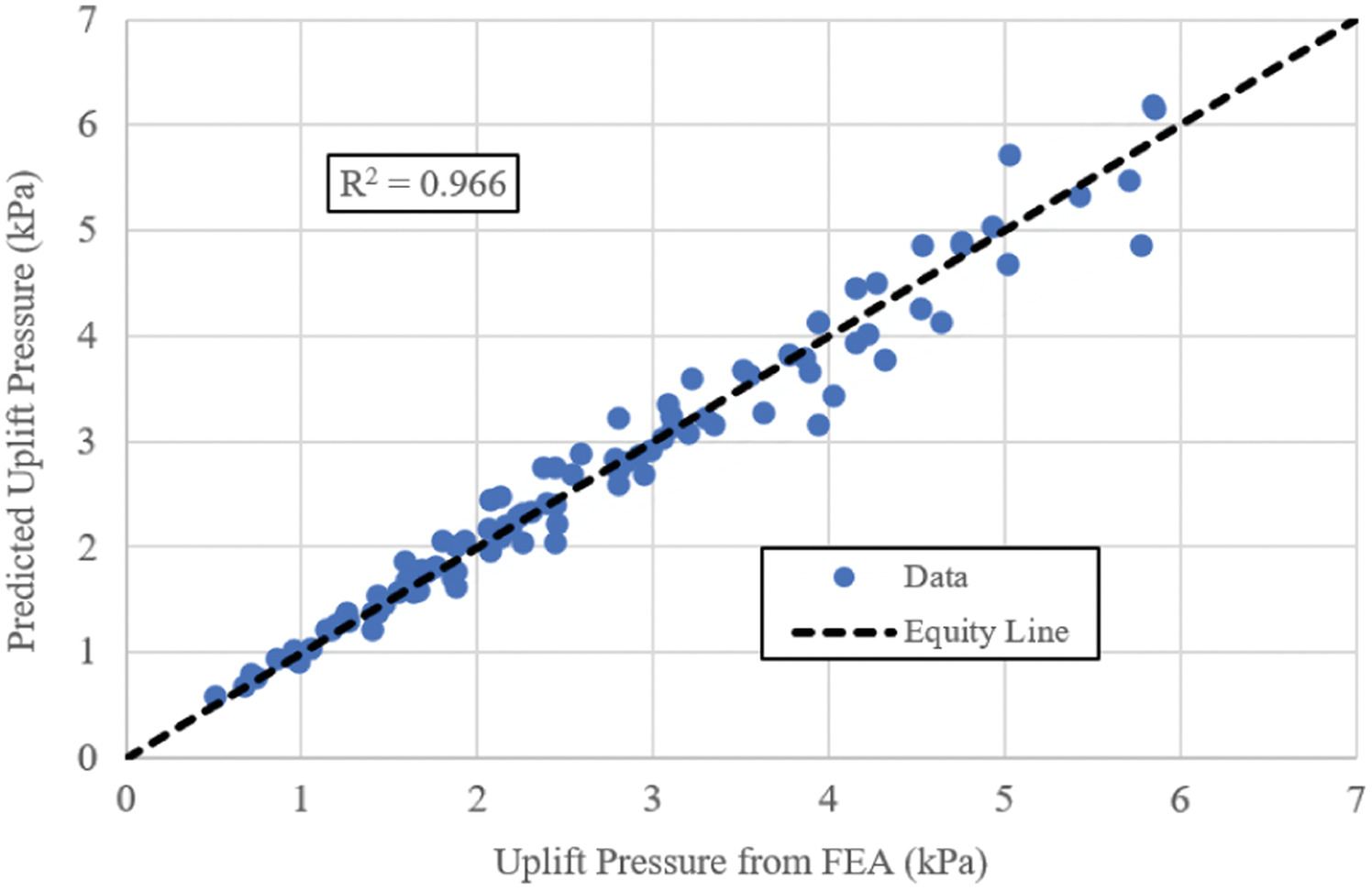
Fig. 7 shows a scatterplot demonstrating that the simplified parametric model is in good agreement with the detailed FEA results, as indicated by the value of 0.967.

For use in the damage modeling, the standing seam metal roof panels attached to plywood roof decks were modeled using 29-gauge metal, with a rib height of 16 mm and a fastener spacing of 610 mm, yielding a mean uplift resistance of 3.8 kPa.
Uplift Resistance of Standing Seam Metal Roofs Connected to Purlins Using Clips
Detailed finite-element models of standing seam metals roofs connected to purlins with clips were developed to evaluate their wind uplift resistances. The finite-element model was utilized to study the influence of several design variables on the uplift resistances such as seam height, metal thickness, fastener spacing, and width of the panel. Based on finite-element analysis responses, parametric equations were developed to model wind uplift resistances of these standing seam metal roofs connected to purlins when subjected to a uniform uplift pressure.
The finite-element models of metal roofs were developed following the techniques presented in El Damatty et al. (2003) and Lovisa et al. (2013). The material properties of metal panels were taken from studies by Ali and Senseny (2003) and El Damatty et al. (2003). The force–displacement responses of the nonlinear springs representing seam and supporting clips were obtained from test results reported by El Damatty et al. (2003) and El Damatty and Rahman (2004). The boundary conditions applied in the simulation of the metal roof were the same as those used by El Damatty et al. (2003) in their studies on standing seam metal roofs.
To validate the finite-element model, a test conducted at Mississippi State University (Sinno et al. 2003) on the static uplift resistance of a standing seam metal roof was used. The test involved attaching a full-scale standing seam roof to a pressure chamber and applying a static uplift pressure. The test was conducted using a 6.43-m-long standing seam metal panel system. Five full-width panels were seamed together to constitute the full-scale test specimen. The roof was supported by a row of clips aligned along the seam line and spaced at 1,550 mm. The clips were in turn supported by purlins aligned in the direction perpendicular to the seams. The purlins were made of rectangular aluminum tubes having a rectangular cross section () and a length of 4 m. The purlins, spaced at 1,550 mm, were supported at their ends to the sides of the test chamber. The load was applied to the roof in the form of a uniform uplift pressure.
In the finite-element model, the standing seam metal panel dimensions and experimental setup were modeled and uniform uplift pressure was applied to evaluate the metal panel’s uplift resistance and the clip reactions. The simulated clip reactions were verified through comparisons with experimental data.
The FEA predicts the experimental uplift resistance and clip reactions reasonably well. The failure in the FEA was due to seam disengagement, which is the same failure mechanism observed in the full-scale experiment by Sinno et al. (2003) and more recently by Wu et al. (2020). This was taken as validation of the finite-element model of the standing seam metal roof, and the model was further utilized to study the influence of different variables on the static uplift resistances of standing seam metal roofs. Several studies demonstrated that the uplift resistances under uniform static pressures are not representative of realistic wind uplift responses of standing seam metal roofs (Farquhar et al. 2005; Habte et al. 2015); however, it has been observed that uplift resistances under static uniform pressure yield more conservative estimates than those obtained using more realistic wind loadings (Habte et al. 2015; Morrison and Reinhold 2015). In addition, use of dynamic wind loads on the standing seam metal roof comes along with several other parameters that must be accounted for such as wind pressures along roof edges and corners (Farquhar et al. 2005), edge restraints (Dixon et al. 2011), and other modes of local failure at the metal clips, which are not considered in the developed models. Therefore, considering the simplicity and conservativeness, the uplift resistances of the standing seam metal roof presented in this paper were developed based on the static uniform uplift pressure instead of more realistic dynamic wind loads.
Uplift resistance of a standing seam metal roof panel was evaluated by changing the seam height, metal panel thickness, purlin spacing, and panel width so the influence of each of these parameters could be investigated and a simple parametric model could be developed to calculate the static uplift resistances for a range of panel widths, purlin spacings, and so on. The width of the panel was varied between 300 and 762 mm with two major corrugations 50–75 mm high along each edge. The thickness of the metal was varied between 0.46 and 0.76 mm, and the purlin spacing was varied between 0.76 and 1.55 m.
The uplift resistance was expressed as a nonlinear function of panel thickness and seam height given aswhere = uplift the resistance (kPa); = panel thickness (mm); and = seam height (mm).
(10)
To calculate uplift resistances for different panel widths and purlin spacing, uplift resistances normalized to the base case (e.g., 610-mm-wide standing seam metal roof with 1,550-mm purlin spacing) were plotted against panel width and purlin spacing. The normalized uplift resistance decreases nonlinearly with increasing panel width and purlin spacing, and hence two adjustment factors were proposed to take into account the effect of panel width and purlin spacing. The expressions for these two adjustment factors are given in Eqs. (11) and (12), respectivelywhere = adjustment factor for panel width; = adjustment factor for purlin spacing; = panel width (mm); and = purlin spacing (mm).
(11)
(12)
By combining Eqs. (10)–(12), uplift resistance of a standing seam metal roof can be calculated using Eq. (13) for different panel thicknesses, seam heights, panel widths, and purlin spacings
(13)
Fig. 8 shows a scatterplot where the FEA simulated responses are plotted against the parametric model.
For use in the damage modeling, the default clipped standing seam metal roofs were modeled using 26-gauge metal, with a rib height of 38 mm and a clip spacing of 610 mm, yielding a mean uplift resistance of 3.1 kPa.
Elastomeric Roof Covers
The elastomeric roof covering model developed for use for residential construction in the USVI comprises a water-resistant coating applied directly onto the wood sheathing. The elastomeric top coat is treated as being 100% waterproof until a roof sheathing panel fails. Because there are no data on the possible progressive failure of elastomeric roof covers due to the failure of a roof panel, it is assumed that the elastomeric roof covering on panels adjacent to a failed roof panel are unaffected by failures of adjacent roof deck elements.
Concrete Roofs
Concrete roofs on residential buildings are modeled as being impervious to water, and do not consider the costs or consequences associated with the failure of a roof membrane (if one exists) covering the concrete roof deck; consequently, the loss model would be expected to underestimate the losses for buildings with concrete roofs because damage to the interior of the building associated with water intrusion is not modeled. Because no detailed analyses were performed to assess the damageability of concrete roofs to wind loads, the concrete roof deck or structure is assumed to not fail at any wind speed considered here, and consequently the effect of roof shape on wind loads is not relevant. These concrete roofed buildings were introduced into Hazus to handle the significant number of houses in Puerto Rico that have flat concrete roofs. The walls of all buildings with concrete roofs are modeled as masonry and can fail. The capacity of the masonry walls was developed using yield line theory as described in FEMA (2021).
Model Buildings Used to Develop Damage Functions
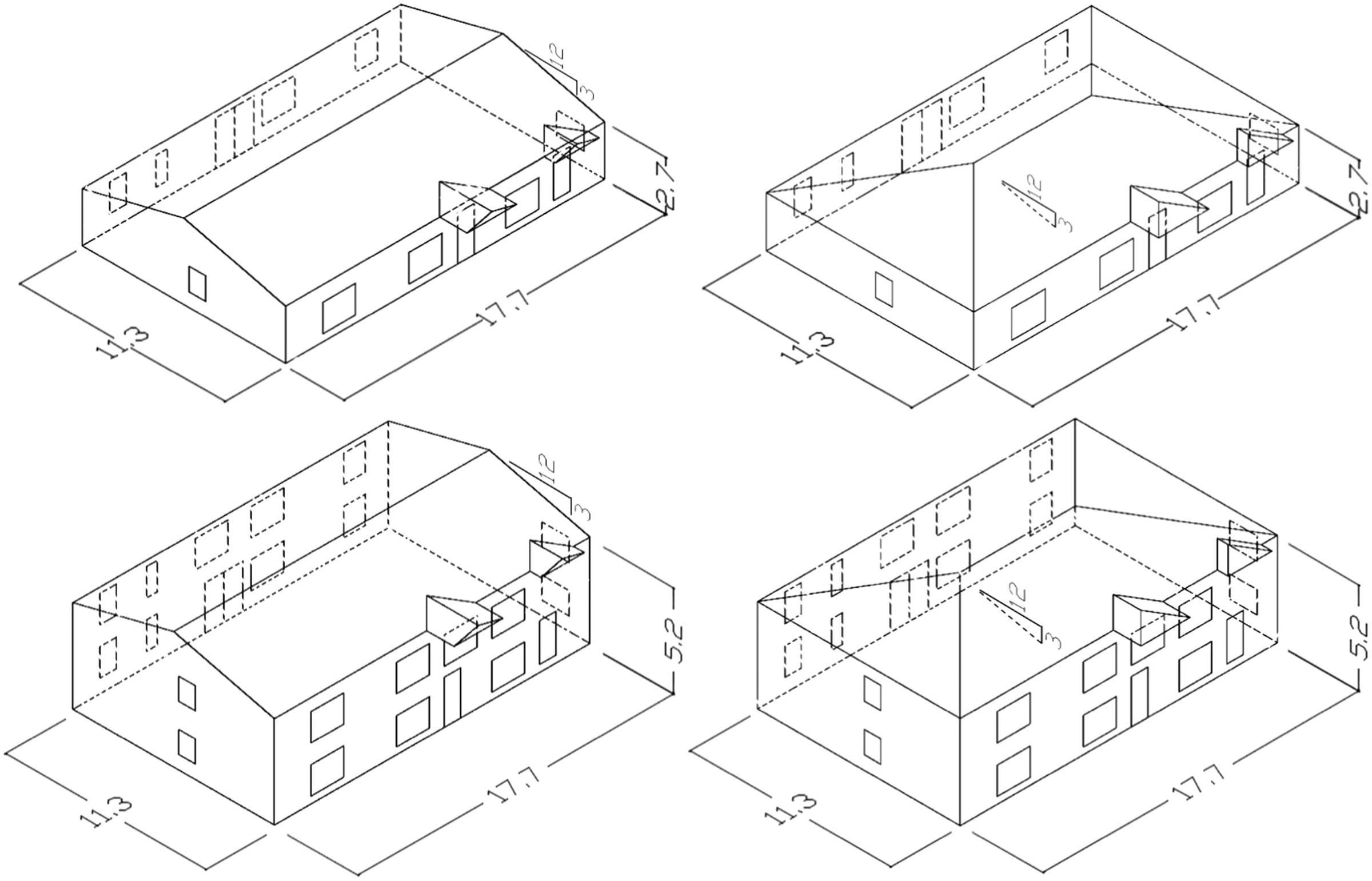
The geometries of the new model buildings used to develop the damage functions for the USVI are presented in Fig. 9. The geometries of the new buildings used to develop the damage functions for PR are given in Fig. 10. The buildings depicted in Figs. 9 and 10 can be used in any location where building characteristics consistent with those modeled here are relevant.

Damage and Loss Modeling
The methodology used herein to develop the building and content loss estimates, building damage estimates, and estimates of building debris is essentially the same as that described in the Hazus Hurricane Model technical manual (FEMA 2021), with differences described in the following.
Damage Modeling
One of the major differences between the methodology used in the development of the original damage, debris, and loss functions is an update to the modeling of the roof pressure coefficients. The roof pressure coefficients used in the development of the original damage/loss functions (FEMA 2021) match those given in ASCE 7-02 (ASCE 2003). The roof pressure coefficients used to develop the damage/loss functions described herein use roof pressure coefficients that are closer to those given in ASCE 7-16 (ASCE 2017) and ASCE 7-22 (ASCE 2022), which are notably higher than those given in ASCE 7-02 (ASCE 2003). Consequently, with all else held constant, it is expected that the damage functions developed herein will yield higher damage and loss for the same wind speed compared to those developed in 2002.
To develop the damage and loss functions, a 100,000-year simulation of hurricane wind speeds and directions was used to generate building damage and loss data on a storm-by-storm basis. The development of the Hazus loss functions given in the original version of Hazus (FEMA 2021) used a 20,000-year simulation developed for Miami. Both sets of loss functions developed here also used simulations performed for a location in Miami because Miami has a higher wind hazard than either the USVI or Puerto Rico, and consequently produces more high-wind-speed storms than would be experienced in the USVI and Puerto Rico, resulting in improved damage and loss estimates for high-wind-speed events. Any small differences in the loss functions associated with differences in hurricane climatology such as storm size, translation speed, and directionality would be excluded. To reduce computational time, a reduced set of events was selected by assigning each event to a wind speed bin based on its maximum overland wind speed. Only 500 storms in each 2.25-m/s bin were saved and used for the prediction of damage. This approach ensures computational effort is not wasted on events that produce very low losses. In total, a maximum of 20,500 storms were retained for use in the damage calculations.
For each storm, 30 replications of building damage were produced. At the start of each replication, resistance values were sampled for each component on the building (e.g., roof deck, roof cover, window resistance, and roof–wall connection). Once all the resistances were assigned, uncertainties in the estimated pressure coefficients and the local wind load sheltering factor were sampled. The error term is an estimate of the differences between full-scale and wind tunnel–derived exterior pressure coefficients. The error term is discussed in more detail in FEMA (2021). A wind load shelter factor (discussed in FEMA 2021) considers the reduction in wind loads due to the effects of sheltering brought about by nearby buildings. The factor was developed using the results of wind tunnel tests where low-rise buildings were tested in open and suburban terrain conditions with and without surrounding buildings in place. These factors were treated as fully correlated over the exterior of the building. After the wind load error terms were sampled, the wind speeds and directions associated with each simulated hurricane were computed every 15 min. Using the wind speed and direction data coupled with the wind loading coefficients, wind loads were computed on each component, and the loads compared to the computed resistances. In addition to the wind loads, windborne debris impacts were computed, and the sampled impact energy was checked against the sampled impact resistance to determine whether a component had failed. The windborne debris model is discussed in detail in FEMA (2021) and Applied Research Associates (ARA) (2008). Upon completion of the failure check for every component, if any components had failed, the internal pressure was recomputed, and each component was checked again to determine whether any additional failures had occurred. This process was repeated until there were no more additional failures. This approach ensures that cascading failures due to windborne debris impacts to fenestrations are properly modeled. A total of 231,000 simulations were performed for each building examined. The resistances used for each component are presented in Table 1. The model buildings used for the development USVI and Puerto Rico building damage functions are shown in Figs. 9 and 10.
| Component | Resistance | Source |
|---|---|---|
| Regular windows | , | FEMA (2021) |
| Jalousie windows (old) | , | Judgment |
| Jalousie windows (new) | , | Acosta and Carandang (2018) |
| Corrugated metal (nailed) | , | FEA |
| Corrugated metal (screwed) | , | FEM analysis |
| Standing seam metal (through fastened) | , | FEM analysis |
| Standing seam metal (clips) | , | FEM analysis |
| Plywood deck (6d with 6/12 spacing) | , | FEMA (2021) |
| Plywood deck (8d with 6/12 spacing) | , | FEMA (2021) |
| Plywood deck (8d with 6/6 spacing) | , | FEMA (2021) |
| Concrete roof deck | N/A—failure not modeled | Judgment |
| Roof–wall (toe-nail) | , | FEMA (2021) |
| Roof–wall (strap/one side wrap) | , | FEMA (2021) |
| Roof–wall (concrete) | , | Judgment |
Damage results from each individual simulation were stored and subsequently used in the calculations for content loss, number of days for reconstruction, and debris. The results, in terms of wind speed dependent averages, are stored in wind speed bins.
Damage results, including the total volume of rainwater entering the building (FEMA 2021), from each individual simulation were stored and subsequently used in the calculations for building loss, content loss, reconstruction time, and debris. The volume of rainwater entering the building is computed by relating the volume of air entering the building with information on the combined wind speed–rainfall rates resulting from the hurricane simulations. Because the Hazus damage function model computes pressures on all fenestrations, once fenestrations(s) fail, the net flow into the building is computed using the continuity equation at each time step. Background leakage was modeled allowing air to enter the building when only a single fenestration fails. The methodology is described in detail in Twisdale et al. (2022).
The results, in terms of wind speed–dependent averages, were stored in wind speed bins.
Loss Modeling
The loss model, which translates physical damage to a financial loss, is similar to that described in FEMA (2021), but it has been updated to include the impact on nonmodeled losses (such as damage to exterior lighting, damaged gutters, and exterior painting) at low wind speeds as discussed in ARA (2008). No changes to the loss model in terms of the relative values of the interior versus exterior of the building were made, nor were there any updates to the assumed vulnerability of the interior of the building due to water intrusion. Wind- and rain-induced losses experienced by a structure were modeled as explicit and implicit losses. Explicit losses include the replacements of those components that are explicitly damaged by the damage model including windows and doors, roof cover, roof sheathing, roof frame, and walls. Implicit damage includes the costs to replace building interiors such as interior walls, flooring, cabinetry, plumbing, electric, and HVAC. The implicit damage model was developed empirically, relating implicit damage to exterior roof deck and roof cover damage and quantitative estimates of water entering the building through broken fenestrations. The relative values of the various components were obtained using RSMeans. The model includes thresholds, after which full replacement will occur. Examples of the thresholds include a maximum percentage of roof shingle loss, after which a full replacement will occur. Other examples include specifying a 100% loss if the roof sheathing damage exceeds 25% or the whole roof fails. The implicit loss functions, as well as some damage thresholds, were developed using insurance company loss data from the mainland United States.
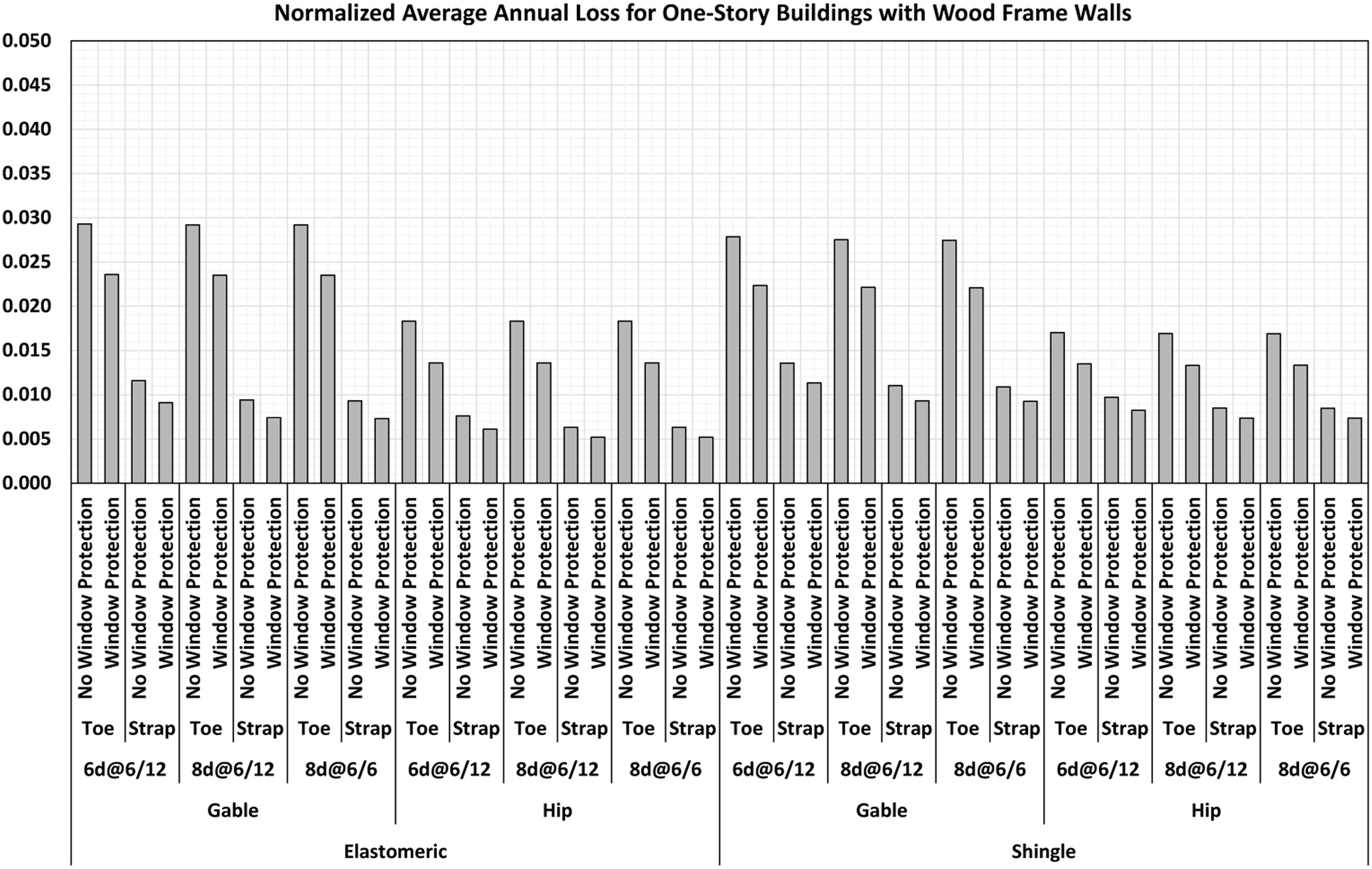
Figs. 11–15 present comparisons of the modeled building loss versus wind speed for various roof types on a one-story, wood-frame, single-family building (WSF1). In all cases, the modeled building loss is compared to the same building with Hazus-standard roof type for reference: a shingled roof where roof sheathing (if applicable) is secured using 8d nails at 150-mm (edge) and 300-mm (field) spacing. The wind speeds are peak (3-s) gust wind speeds at a height of 10 m in open terrain. The buildings are situated in suburban terrain and are modeled with a surface roughness of 0.35 m.

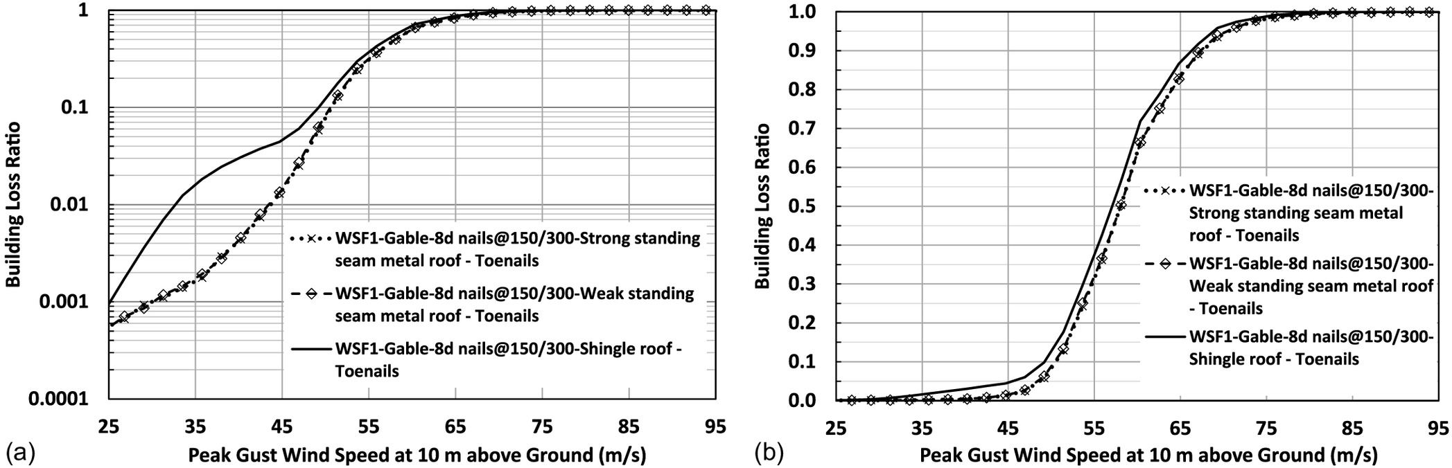
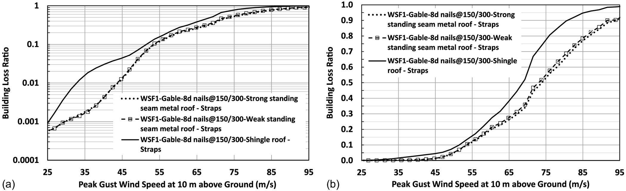
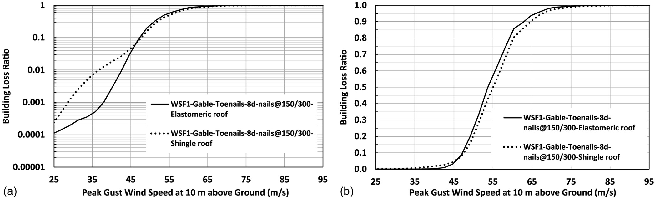
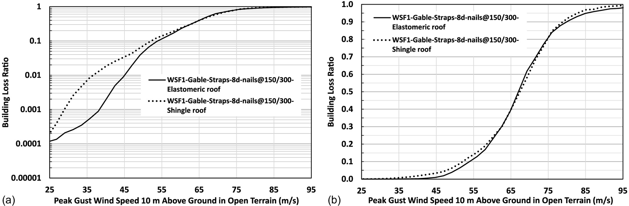
The loss curves in Figs. 11–15 are presented in two different formats, with the data in Figs. 11(a), 12(a), 13(a), 14(a), and 15(a) providing the mean losses on a logarithmic scale and Figs. 11(b), 12(b), 13(b), 14(b), and 15(b) providing the same losses on an arithmetic scale. The logarithmic plots highlight the differences in the loss functions at low wind speeds (less than ).
Fig. 11 presents the losses associated with one-story, wood-frame houses roofed with corrugated metal. The roof framing is attached to the exterior walls using toe-nailed connections. The model buildings having corrugated roofs are designed to be representative of informal construction. The corrugated metal acts as both the roof membrane and the roof sheathing; thus, if one corrugated metal panel fails, significant water damage will occur. The results show the buildings having corrugated metal roofs are significantly more vulnerable than those with the shingles attached to a plywood roof deck, except for very low wind speeds, where failed shingles at low wind speeds produce damage and loss that does not occur with the metal roof cases. The plywood roof deck for the shingle case is modeled as having been attached to the roof trusses using 8d nails.
Figs. 12 and 13 present the loss functions for the standing seam metal roof cases for toe-nailed and strapped roof–wall connection cases, respectively. In the toe-nail case, no difference is seen in the performance of the weak (clipped) or strong (through fastened) standing seam metal roof connections because the entire roof fails before the roof cover itself fails. The shingled roof house produces higher losses than the standing seam metal roof cases for all wind speeds and both roof–wall connection cases because the standing seam metal roofs perform better than shingles. This is particularly evident at low wind speeds where shingles fail but the standing seam metal roofs do not. The higher losses at low wind speeds are attributed to the cost required to replace the scattered shingles that fail. In the strapped roof–wall connection case, the same behavior is observed at low wind speeds () as the toe-nail roof case.
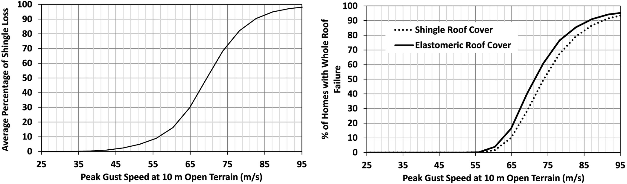
Figs. 14 and 15 present comparisons of the modeled performance of the shingle roof buildings and those with an elastomeric roof cover for toe-nailed and strapped roof–wall connection cases, respectively. The roof deck for both buildings is plywood connected to trusses using 8d nails using a pattern. In both cases, for wind speeds less than approximately , the shingled roof building yields higher losses owing to the cost of repairing or replacing scattered shingle damage. For higher wind speeds, the performance of the entire roof system appears to be the dominant cause of the difference in the performance of the buildings with the different roof covers. Fig. 16 presents comparisons of the roof cover damage (shingles only) and whole roof failures for the elastomeric and shingled roof cases. If the whole roof fails then the shingle loss is set to 100% and is reflected in the average percentage of shingle loss shown in Fig. 16(a). A comparison of the whole roof failures indicates the additional self-weight associated with the shingles reduces whole roof failures, but the additional costs associated with replacing shingles in cases where the whole roofs fails offsets the savings brought about by the reduced whole roof failures.
To provide a quick comparison of the relative performance (or strength) of the buildings having various attributes, the average annual losses of all buildings with all combinations of building characteristics (e.g., roof covers, window protection, roof–wall connections) examined were developed. The average annual losses were computed by applying the Miami climatology to the Caribbean building stock.
Examples presenting the normalized average (normalized by the structure value) annual losses (AAL) for a subset of the combinations for which loss estimates were produced. Fig. 17 presents the AALs for one of the standing seam metal roof cases. Results are given for the wood-frame construction case and show the relative effect of roof shape, roof–wall connection, roof sheathing attachment, window type, and metal roof-to-sheathing connection. The data presented in Fig. 16 indicate that the largest reduction in AAL is due to the use of straps for the roof–wall connection rather than toe-nails. The introduction of window protection produces the second largest reduction in AAL. The effect on AAL due to window type is relatively small, with the jalousie window (J) yielding slightly lower losses than the “regular” (R) window. Similarly, the use of exposed screws to attach the standing seam metal roof cover yields only a small reduction in AAL compared to the clip case. The AALs for the unreinforced masonry (URM) construction case are, on average, 4.5% lower than those using wood-frame construction.
Fig. 18 presents the normalized AALs for all the corrugated roof cases (the only roof–wall connection modeled was toe-nail). The results indicate that the biggest reduction in AAL is due to the use of screws instead of nails to attach the corrugated metal roofing to the battens. The use of window protection to reduce AALs is not as effective as in the case of standing metal roofs owing to whole roof and roof decking failures occurring at wind speeds lower than those associated with significant debris impact. The effect of window type is small, with the jalousie windows associated with slightly lower AALs. As is the case with all building types, the two-story buildings have higher AALs than one-story buildings, and hip roofed buildings yield lower AALs than the gabled roof cases. Comparing the AALs for the corrugated roof case to those presented for the standing seam metal roof case, it is seen that the corrugated metal roof AALs are more than double those for the standing seam metal roof cases.

Fig. 19 presents the normalized AALs for all the concrete roof cases, where it is evident that the AALs for the concrete roofed buildings are lower than those of any of the other cases. Here the AALs are higher in the two-story cases owing to the two-story houses having more windows than the one story. Because the window pressures are referenced to the dynamic wind pressure at mean roof height, which is higher for two-story buildings, the window pressures are higher. Here, the jalousie windows yield higher AALs than the regular window cases.
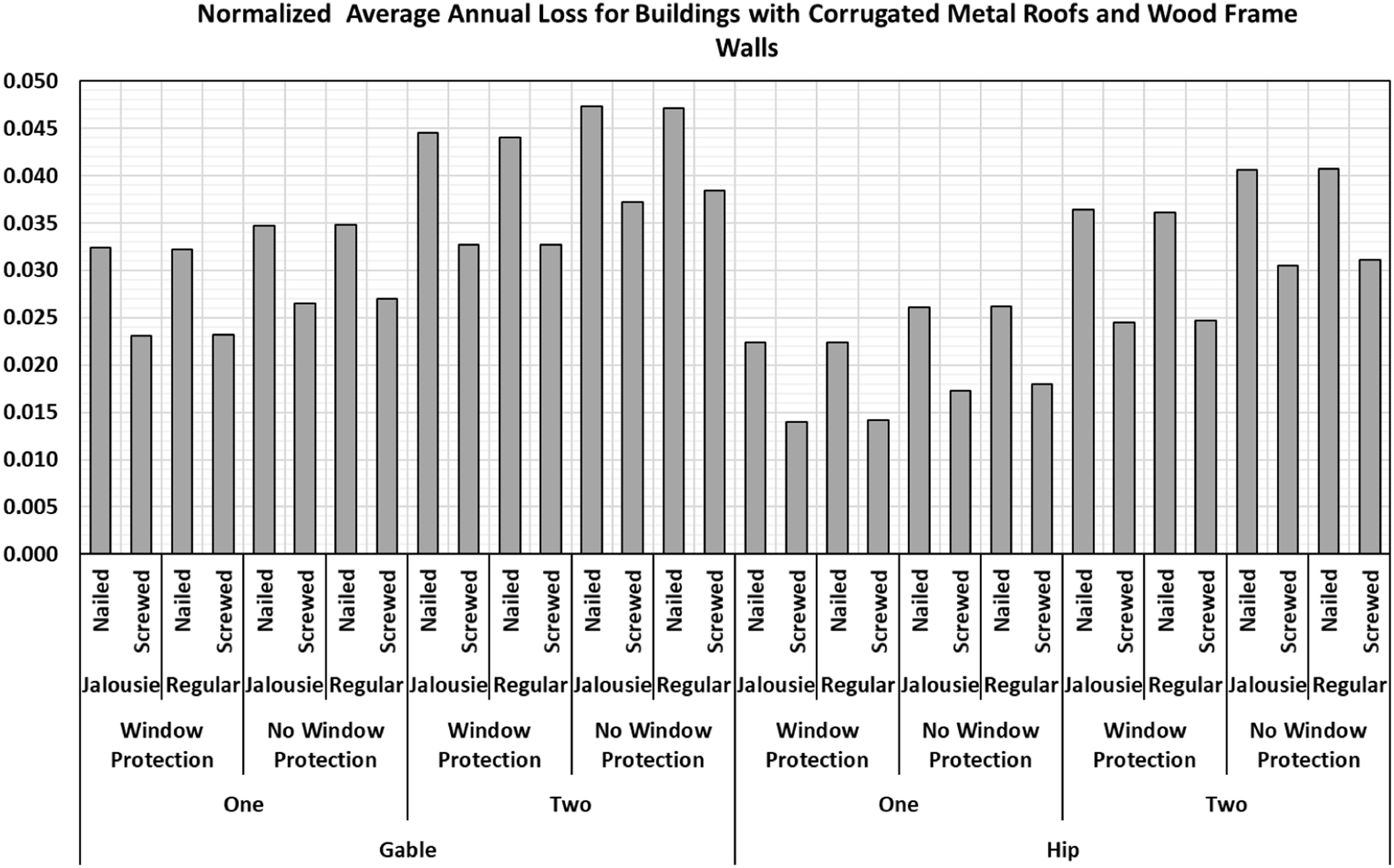
Fig. 20 presents the normalized AALs comparing the AALs for elastomeric roof cover cases to the shingle roof cases (one-story wood-frame construction). Recall the shingled building AALs were computed using the wind load, damage, and loss models used to develop the loss functions for the 2002 version of Hazus, which are still in use. Consequently, differences between the AALs for the shingle and elastomeric roof cases arise from both changes in the modeling as well as changes due to building performance. The decrease in AAL associated with upgrading from toe-nailed roof–wall connections to strapped connections is greater for the elastomeric roof cases because the elastomeric roof cover provides less dead weight, resulting in whole roofs failing at lower wind speeds than in the case of a shingled roof. Consequently, the use of straps increases the failure wind speed; hence, roof failures occur less frequently. As seen in other examples, AALs are lower for hip roofed buildings. Comparing the standing seam metal roof cover AALs to those with elastomeric roof covers, it is seen that the standing seam metal roof covers perform better.

Conclusions
The Hazus Hurricane Model has been extended to include the US Virgin Islands and Puerto Rico. The Hurricane Hazard Model uses the same model incorporated into the ASCE 7-22 wind hazard maps for the US mainland and the US Caribbean islands; however, the validity of the Hurricane Model for use in the Caribbean is documented here for the first time. New damage functions were developed to model construction material and characteristics used in the islands that are different from those used in the mainland United States. Using finite-element analyses, capacity models were developed for corrugated metal roofs and standing seam metal roofs. In both cases parametric models were developed that can be used by others to compute the uplift capacity of the metal panels for various combinations of fastener types, fastener spacings, gauges of metal, and sizes of the panels; however, because data on the actual values used in the region were not available, only one value of thickness, spacing, and so on (Table 1) was used for each metal roof cover type modeled herein. The new version of Hazus (version 5.0) containing the US Caribbean model was released in May 2021.
Data Availability Statement
Some or all data, models, or code generated or used during the study are available from the authors upon reasonable request. The Hazus software is able at the following link: https://www.fema.gov/flood-maps/tools-resources/flood-map-products/hazus/software.
Acknowledgments
This work was supported by the Federal Emergency Management Agency (FEMA) under Contracts HSFE60-15-D-0003 and HSFE60-15-D-0005. Any opinions, findings, and conclusions or recommendations expressed in this paper are those of the authors and do not necessarily reflect the views of FEMA.
References
Acosta, T. J., and A. J. Carandang. 2018. “Experimental investigation of jalousie type wind frames subjected to static wind pressure.” Philipp. Eng. J. 39 (2): 75–88.
Ali, H. M., and P. E. Senseny. 2003. “Models for standing seam roofs.” J. Wind Eng. Ind. Aerodyn. 91 (12–15): 1689–1702. https://doi.org/10.1016/j.jweia.2003.09.014.
ARA (Applied Research Associates). 2008. 2008 Florida residential wind loss mitigation study, Florida Office of insurance regulation contract number IR018 October 2008. Raleigh, NC: ARA.
ASCE. 2003. Minimum design loads and associated criteria for buildings and other structures. ASCE/SEI 7-02. Reston, VA: ASCE.
ASCE. 2017. Minimum design loads and associated criteria for buildings and other structures. ASCE/SEI 7-16. Reston, VA: ASCE.
ASCE. 2022. Minimum design loads and associated criteria for buildings and other structures. ASCE/SEI 7-22. Reston, VA: ASCE.
DeMaria, M., and J. Kaplan. 1999. “An updated statistical hurricane intensity prediction scheme (SHIPS) for the Atlantic and Eastern North Pacific Basins.” Weather Forecasting 14 (3): 326–337. https://doi.org/10.1175/1520-0434(1999)014%3C0326:AUSHIP%3E2.0.CO;2.
Dixon, C., D. Prevatt, and P. Datin. 2011. “Influence of edge restraint on clip fastener loads of standing seam metal roof panels.” J. ASTM Int. 8 (8): 103704. https://doi.org/10.1520/JAI103704.
Doudak, G. 2005. “Field determination and modeling of load paths in wood light-frame structures.” Doctoral dissertation, Dept. of Civil Engineering, McGill Univ.
El Damatty, A. A., and M. Rahman. 2004. “Testing and analysis for non-linear behavior of standing seam roof.” In Proc., 4th Int. Conf. on Thin-Walled Structures. Bristol, UK: IOP Publishing.
El Damatty, A. A., M. Rahman, and O. Ragheb. 2003. “Component testing and finite element modeling of standing seam roofs.” Thin-Walled Struct. 41 (11): 1053–1072. https://doi.org/10.1016/S0263-8231(03)00048-X.
Emanuel, K. A., S. Ravela, E. Vivant, and C. Risi. 2006. “A statistical–deterministic approach to hurricane risk assessment.” Bull. Am. Meteorol. Soc. 87 (3): 299–314. https://doi.org/10.1175/BAMS-87-3-299.
ESDU (Engineering Sciences Data Unit). 1982. Strong winds in the atmospheric boundary layer, Part 1: Mean hourly wind speed. London: ESDU.
ESDU (Engineering Sciences Data Unit). 1983. Strong winds in the atmospheric boundary layer, Part 2: Discrete gust speeds. London: ESDU.
Farquhar, S., G. A. Kopp, and D. Surry. 2005. “Wind tunnel and uniform pressure tests of a standing seam metal roof model.” J. Struct. Eng. 131 (4): 650–659. https://doi.org/10.1061/(ASCE)0733-9445(2005)131:4(650).
FEMA. 2021. Multi-hazard loss estimation methodology hurricane model Hazus—MH 2.1 technical manual. Washington, DC: FEMA.
Georgiou, P. N. 1985. “Design windspeeds in tropical cyclone-prone regions.” Ph.D. thesis, Faculty of Engineering Science, Univ. of Western Ontario.
Georgiou, P. N., A. G. Davenport, and B. J. Vickery. 1983. “Design wind speeds in regions dominated by tropical cyclones.” J. Wind Eng. Ind. Aerodyn. 13 (1–3): 139–152.
Gringorten, I. I. 1963. “A plotting rule for extreme probability paper.” J. Geophys. Res. 68 (3): 813–814. https://doi.org/10.1029/JZ068i003p00813.
Habte, F., M. A. Mooneghi, A. G. Chowdhury, and P. Irwin. 2015. “Full-scale testing to evaluate the performance of standing seam metal roofs under simulated wind loading.” Eng. Struct. 105 (Dec): 231–248. https://doi.org/10.1016/j.engstruct.2015.10.006.
Holland, G. 1980. “An analytic model of the wind and pressure profiles in hurricanes.” Mon. Weather Rev. 108: 1212–1218.
Kumar, N., V. Dayal, and P. P. Sarkar. 2012. “Failure of wood-framed low-rise buildings under tornado wind loads.” Eng. Struct. 39 (Jun): 79–88. https://doi.org/10.1016/j.engstruct.2012.02.011.
Lovisa, A. C., V. Z. Wang, D. J. Henderson, and J. D. Ginger. 2013. “Development and validation of a numerical model for steel roof cladding subject to static uplift loads.” Wind Struct. Int. J. 17 (5): 495–513. https://doi.org/10.12989/was.2013.17.5.495.
Mahendran, M. 1990. “Static behaviour of corrugated roofing under simulated wind loading.” Trans. Inst. Eng. Aust. Civ. Eng. 32 (4): 212–218.
Mahendran, M. 1992. “Contrasting behaviour of thin steel roof claddings under simulated cyclonic wind loading.” In Proc., 11th Int. Specialty Conf. on Cold-Formed Steel Structures, 245–256. Rolla, MO: Univ. of Missouri-Rolla.
Mahendran, M. 1994. “Behaviour and design of crest-fixed profiled steel roof claddings under wind uplift.” Eng. Struct. 16 (5): 368–376. https://doi.org/10.1016/0141-0296(94)90030-2.
Martin, K. G., R. Gupta, D. O. Prevatt, P. L. Datin, and J. W. van de Lindt. 2011. “Modeling system effects and structural load paths in a wood-framed structure.” J. Archit. Eng. 17 (4): 134–143. https://doi.org/10.1061/(ASCE)AE.1943-5568.0000045.
Morrison, M. J., and T. A. Reinhold. 2015. “Performance of metal roofing to realistic wind loads and evaluation of current test standards.” In Proc., 14th Int. Conf. on Wind Engineering, 21–26. Kanagawa, Japan: International Association for Wind Engineering.
Pan, F., C. S. Cai, and W. Zhang. 2013. “Refined finite element modeling of a typical low-rise building for damage predictions under hurricane loads.” In Proc., 12th Americas Conf. on Wind Engineering (12ACWE), Ames, IA: International Association for Wind Engineering.
Roy, K., J. B. P. Lim, A. M. Yousefi, G. C. Clifton, and M. Mahendran. 2018. “Low fatigue response of crest-fixed cold-formed steel drape curved roof claddings.” In Proc., Int. Specialty Conf. on Cold-Formed Steel Structures, 4. Rolla, MO: Univ. of Missouri-Rolla.
Sinno, R. R., D. Surry, S. Fowler, and T. C. E. Ho. 2003. “Testing of metal roofing systems under simulated realistic wind loads.” In Proc., 11th Int. Conf. on Wind Engineering, 1065–1072. Kanagawa, Japan: International Association for Wind Engineering.
Sivapathasundaram, M., and M. Mahendran. 2018. “New pull-out capacity equations for the design of screw fastener connections in steel cladding systems.” Thin-Walled Struct. 122 (Mar): 439–451. https://doi.org/10.1016/j.tws.2017.08.019.
Thampi, H. 2010. “Interaction of a translating tornado with low-rise building.” M.S. thesis, Dept. of Civil, Construction and Environmental Engineering, Iowa State Univ.
Twisdale, L. A., S. Banik, L. Mudd, S. Quayyum, F. Liu, M. Faletra, P. J. Vickery, M. L. Levitan, and L. Phan. 2022. Tornado wind speed risk maps for building design. Technical Note. Gaithersburg, MD: National Institute of Standards and Technology.
Vickery, P. J. 2005. “Simple empirical models for estimating the increase in the central pressure of tropical cyclones after landfall along the coastline of the United States.” J. Appl. Meteorol. 44 (12): 1807–1826. https://doi.org/10.1175/JAM2310.1.
Vickery, P. J., F. A. Liu, and J. X. Lin. Forthcoming. “Development of topographic wind speed-ups and hurricane hazard maps for Puerto Rico.” J. Struct. Eng.
Vickery, P. J., P. F. Skerlj, J. Lin, L. A. Twisdale Jr., M. A. Young, and F. M. Lavelle. 2006. “HAZUS-MH hurricane model methodology. II: Damage and loss estimation.” Nat. Hazards Rev. 7 (2): 94–103. https://doi.org/10.1061/(ASCE)1527-6988(2006)7:2(94).
Vickery, P. J., P. F. Skerlj, and L. A. Twisdale Jr. 2000. “Simulation of hurricane risk in the US using empirical track model.” J. Struct. Eng. 126 (10): 1222–1237. https://doi.org/10.1061/(ASCE)0733-9445(2000)126:10(1222).
Vickery, P. J., and L. A. Twisdale. 1995. “Prediction of hurricane wind speeds in the United States.” J. Struct. Eng. 121 (10): 1691–1699. https://doi.org/10.1061/(ASCE)0733-9445(1995)121:11(1691).
Vickery, P. J., and D. Wadhera. 2008. “Statistical models of Holland pressure profile parameter and radius to maximum winds of hurricanes from flight level pressure and H*wind data.” J. Appl. Meteorol. 47 (10): 2497–2517. https://doi.org/10.1175/2008JAMC1837.1.
Vickery, P. J., D. Wadhera, M. D. Powell, and Y. Chen. 2009a. “A hurricane boundary layer and wind field model for use in engineering applications.” J. Appl. Meteorol. 48 (2): 381–405. https://doi.org/10.1175/2008JAMC1841.1.
Vickery, P. J., D. Wadhera, L. A. Twisdale Jr., and F. M. Lavelle. 2009b. “U.S. hurricane wind speed risk and uncertainty.” J. Struct. Eng. 135 (3): 301–320. https://doi.org/10.1061/(ASCE)0733-9445(2009)135:3(301).
Wu, T., S. Ying, Z. Cao, Z. Yu, and W. Yue. 2020. “Study on the wind uplift failure mechanism of standing seam roof system for performance-based design.” Eng. Struct. 225 (Dec): 111264. https://doi.org/10.1016/j.engstruct.2020.111264.
Xu, Y. L., and G. F. Reardon. 1993. “Test of screw fastened profiled roofing sheets subject to simulated wind uplift.” Eng. Struct. 15 (6): 423–430. https://doi.org/10.1016/0141-0296(93)90060-H.
Xu, Y. L., and J. G. Teng. 1994. “Local plastic failure of light gauge steel roofing sheets: Finite element analysis versus experiment.” J. Constr. Steel Res. 30 (2): 125–150. https://doi.org/10.1016/0143-974X(94)90047-7.
Information & Authors
Information
Published In

Natural Hazards Review
Volume 24 • Issue 4 • November 2023
Copyright
This work is made available under the terms of the Creative Commons Attribution 4.0 International license, https://creativecommons.org/licenses/by/4.0/.
History
Received: Mar 7, 2022
Accepted: Mar 24, 2023
Published online: Jul 14, 2023
Published in print: Nov 1, 2023
Discussion open until: Dec 14, 2023
ASCE Technical Topics:
- Construction engineering
- Construction methods
- Continuum mechanics
- Disaster risk management
- Disasters and hazards
- Dynamic loads
- Dynamics (solid mechanics)
- Engineering fundamentals
- Engineering mechanics
- Finite element method
- Geographic information systems
- Geology
- Geomatics
- Geotechnical engineering
- Hurricanes, typhoons, and cyclones
- Islands
- Methodology (by type)
- Natural disasters
- Numerical methods
- Solid mechanics
- Structural dynamics
- Structural engineering
- Surveying methods
- Wind engineering
- Wind loads
- Wind speed
Authors
Metrics & Citations
Metrics
Citations
Download citation
If you have the appropriate software installed, you can download article citation data to the citation manager of your choice. Simply select your manager software from the list below and click Download.
Cited by
- Francis M. Lavelle, David R. Mizzen, Andrea M. Jackman, Douglas Bausch, Peter J. Vickery, Jesse Rozelle, Maureen E. Kelly, Casey Zuzak, Hurricane Wind Loss Estimation for Puerto Rico and the US Virgin Islands: Model Implementation and Validation, Natural Hazards Review, 10.1061/NHREFO.NHENG-1638, 24, 4, (2023).