Estimating Pluvial Depth–Damage Functions for Areas within the United States Using Historical Claims Data
Abstract
Flooding has been the most costly natural disaster over the last 2 decades within the US. Therefore, recent research has focused on more accurately predicting economic losses from flooding to aid decision makers and mitigate economic exposure. For this, depth–damage functions have commonly been employed to predict the relative or absolute damage to buildings caused by different magnitudes of flooding. Although depth–damage functions, such as those adopted by the US Army Corps of Engineers, are widely available for fluvial and coastal flooding, less work has been done to develop functions for pluvial-induced flooding. Here, we use a database containing 13.5 million claims to develop pluvial depth–damage functions. For this, recently released flood hazard data are utilized to identify claims within the database that are likely related to pluvial flooding. We employed two types of regression models to fit the depth–damage functions. Secondarily, we developed an automated valuation model (AVM) to estimate building values across the state of New Jersey. These building values were then combined with flood hazard layers in order to apply the depth–damage functions and compute an aggregate annualized loss for New Jersey. The results indicated moderate agreement between the observed damage within the state of New Jersey and that computed by applying the study-developed depth–damage curves to buildings within the state using pluvial flood hazard layers. It is anticipated that the depth–damage functions developed by this research will aid future work in more accurately quantifying the economic risks associated with flooding across the US.
Practical Applications
This research included in this paper aimed to develop a practical tool for the estimation of losses from heavy rainfall–driven flood events. Although established models exist to estimate losses from river and surge flooding, rainfall-driven flood damages are not as well understood. In order to estimate these losses, we also developed a property characteristic–driven valuation model. The production of the model gives us a property value baseline to estimate the rainfall losses against our derived damage curves. Our hope is that planners, researchers, and others may use this to estimate losses to properties from extreme rainfall events, which in turn can help to inform the allocation of resources in protecting against those events.
Introduction and Background
Flooding is the most costly natural disaster in the US; floods were responsible for $ 8t billion in economic losses annually from 2000 to 2019 (Smith 2020). The economic costs associated with floods have increased substantially in recent decades within the US and are anticipated to increase further in the future due to the combined effects of urbanization (Cutter et al. 2018) and a changing climate that includes impacts such as sea level rise and an intensification of the hydrologic cycle (Hayhoe et al. 2018). As such, it is anticipated that the importance of flood risk management will increase in the future (Van Ootegem et al. 2015).
An essential component of flood risk management is quantifying future economic flood losses to inform decision makers (e.g., government officials) of the locations that are the most at risk. Currently, depth–damage functions are typically used for these analyses, which are designed to relate building or content damage—relative or absolute—to flood depths (e.g., US Army Corps of Engineers (USACE 2019). Although these functions are widely used to estimate damage associated with coastal and riverine (i.e., fluvial) flooding, depth–damage functions for pluvial, or rainfall-related flooding, are not widely available.
In general, pluvial flooding occurs when high-intensity rainfall results in precipitation accumulation that exceeds the capacity of natural and engineered drainage systems to absorb water or carry it away. Unlike riverine and coastal flooding, pluvial flooding can occur in locations far away from bodies of water. Additionally, pluvial flooding is particularly, and increasingly, challenging to major cities and urban areas characterized by growing populations, impervious surfaces, and aging drainage systems (National Academies of Sciences, Engineering, and Medicine 2019).
Historically, pluvial flood risk has not been well-understood. This is partly due to the complex topographic and drainage dynamics required to accurately model the hazard. Rainfall events that result in pluvial flooding are also difficult to monitor because these events can occur over short time frames and small spatial scales (Rosenzweig et al. 2018). As such, pluvial flood risk has typically been excluded from flood risk analyses (National Academies of Sciences, Engineering, and Medicine 2019). For example, FEMA’s Flood Insurance Rate Maps (FIRMs), which are the most widely used flood risk assessment and communication tools in the US, exclude pluvial flood risk. As a result of this exclusion, Wing et al. (2018) concluded that the inadequate assessment of pluvial flood risk in urban areas has caused FEMA to significantly underestimate the population exposed to flood risk. As a result, many households and communities at risk of pluvial flooding are unaware of it and of the potential economic losses associated with flooding.
Although greater economic damage generally results from a singular riverine or coastal flooding event when compared with a singular pluvial event, the occurrence of riverine and coastal events are relatively rare compared with pluvial events. Over long time frames, research indicated that the cumulative damage associated with pluvial floods is comparable to that of riverine flooding (Zhou et al. 2012). Recent events illustrate the importance of understanding the economic risks associated with pluvial flooding. For example, Hurricane Harvey (2017)—a predominantly pluvial event—dropped more than 150 cm (60 in.) rain on the Houston, Texas, area. The storm killed 68 people and resulted in $125 billion in damages (Blake and Zelinsky 2018). In July 2016, 150 cm (60 in.) of rain fell on Ellicott City, Howard County, Maryland, resulting in flash floods that caused more than $22 million in damages. Less than 2 years later, in May 2018, the city was impacted by a 1-in-1,000-year event in which successive thunderstorms poured 20 cm (8 in.) of rain on the city in just 3 h (Viterbo et al. 2020). The development of depth–damage functions for pluvial flooding could assist stakeholders in providing a more comprehensive view of future flood damage in the US.
Recent research has focused on the development of damage models for pluvial flooding; however, progress has been hindered by the availability of pluvial flood risk data and the lack of damage records for pluvial events (e.g., Van Ootegem et al. 2015; Rözer et al. 2019). Van Ootegem et al. (2015) developed multivariate models using self-reported (i.e., survey) hazard (i.e., flood depths) and nonhazard (e.g., structure type) data to predict building-level economic loss from pluvial flooding in Belgium. Their results indicated that although inundation depth is the most important predictor of damage, nonhazard data are important predictors of economic damage from pluvial flooding (Van Ootegem et al. 2015). In a similar study, Rözer et al. (2019) used survey data to develop probabilistic multivariable models to estimate pluvial flood losses to buildings in Harris County, Texas, impacted by Hurricane Harvey. In agreement with Van Ootegem et al. (2015), the results of Rözer et al. (2019) indicated that the inclusion of nonhazard data reduced the magnitude of uncertainty in flood loss estimates. Although the results of these studies indicate increased utility of depth–damage models by including nonhazard data, both studies noted that this type information is not available for broader scale analyses, and the efficacy of their models is unknown for other regions (Van Ootegem et al. 2015; Rözer et al. 2019).
Given the lack of available data needed for the development of pluvial damage models, several studies have attempted to adapt fluvial depth–damage functions to estimate pluvial flood damage by combining them with the output of urban drainage models (e.g., Freni et al. 2010; Olsen et al. 2015; Zhou et al. 2012). However, the utility of coastal and fluvial functions for understanding economic risk from pluvial flooding remains unclear (e.g., Kellens et al. 2013). Pluvial floods are generally characterized by shorter duration and slower water velocities when compared with fluvial floods (ten Veldhuis 2011). As such, using a curve developed for fluvial flooding to estimate damage for pluvial flooding could lead to systematic biases in loss estimates.
Recently released flood risk data from the First Street Foundation’s flood model (i.e., Bates et al. 2020) provide probabilistic estimates of pluvial flood risk (in addition to fluvial, tidal, and surge risk) for every property parcel in the contiguous US. Given the high spatial resolution of these data, researchers and practitioners can not only communicate pluvial risk at finer spatial scales, but also use these data to estimate expected flood damages at the property level, as Armal et al. (2020) have done for fluvial and coastal flood damages in New Jersey. Additionally, computational advancements have made it possible to examine a large historical claims database, which contains building-level damage assessments and inundation depths, at relatively little computational cost. Therefore, the research presented here aims to contribute to the body of research examining the economic risks associated with pluvial flooding within the US by developing univariate depth–damage functions for pluvial flooding. A secondary goal is to measure external validity through demonstrating the utility of these functions by applying them to areas within the state of New Jersey. For this, an automated valuation model (AVM) was developed to compute building value estimates, which were then used in conjunction with pluvial flood hazard layers and the study-developed depth–damage functions to estimate the annual economic impact from pluvial flooding to buildings within the state. It is anticipated that when combined with recently released flood hazard data, the study-developed pluvial depth–damage functions will afford more holistic economic risk analyses of flood exposure within the contiguous US.
Methods
In developing a pluvial-centered damage function, this research relied on publicly available resources from FEMA, the National Oceanic and Atmospheric Administration (NOAA) (NOAA 2020), and USDA (2020) for data selection and curve refinement. Our estimation of damage followed the methodology used to create the USACE curves in the HAZUS methodology [Armal et al. (2020) has given a review]. Finally, once the damage curves were derived, estimates of economic impacts were computed using a parcel-level building structure AVM. Details of these methods follow here.
Data
Claims Database
The Individual Assistance Housing Registrants—Large Disasters (IA) claims database was downloaded from FEMA (Table 1). This database contains 13.5 million assistance records for the time period between January 2004 and December 2018. Each record represents an individual household’s request for federal aid to assist paying for damage caused by a natural disaster for which a presidential declaration was declared. This data set contains the following relevant fields: ZIP code tabulation area (ZCTA) of the impacted property, total depth of water in the damaged dwelling, the real property damage amount as observed by FEMA, and the year of loss. Additional data set information has been given by Kousky et al. (2018).
Additionally, the National Flood Insurance Program’s (NFIP) claims transaction database was gathered from the Federal Insurance and Mitigation Agency (FIMA) (Table 1). This database contains 2.44 million claims records for the 1970 to 2019 period; however, only claims for the 2004–2018 period were gathered for the research presented here for data completeness and because flooding frequencies accelerated significantly in the mid-2000s (McAlpine and Porter 2018). Each claim record represents an insurance claim on a property that is located within FEMA’s special flood hazard layer and for which there is an active NFIP policy. Of particular interest for this research is that each claim is tagged to the ZCTA in which the impacted building is located, the year during which the loss occurred, and the amount paid by FIMA for the building claim. However, the water depth associated with the claim is not available within this publicly available database. As such, this database will only be used in the case study portion of this analysis.
Flood Risk Data
Because the primary goal of this research is to develop pluvial depth–damage functions, several data sets were downloaded to identify ZCTAs within the contiguous US that have likely only experienced pluvial flooding. These included pluvial and fluvial flood risk data from First Street Foundation (FSF) (Bates et al. 2020) and storm surge data from NOAA (Zachry et al. 2015). Specifically, the 0.2% (i.e., 1-in-500-year flood) fluvial and pluvial flood hazard layers were gathered from FSF (Table 1). These hazard layers are available for the conterminous US at a 3-m spatial resolution; however, for computational tractability, each layer was resampled to a 30-m spatial resolution.
The Category 4 hurricane maximum of maximum (MOM) high-tide hazard layer was gathered from NOAA’s National Hurricane Center (NHC) (Table 1). This inundation layer, which is available at a 30-m spatial resolution, was computed by utilizing the hydrodynamic sea, lake, and overland surges from hurricanes (SLOSH) model to simulate inundation layers for thousands of hypothetical tropical cyclones (Zachry et al. 2015). For each pixel, the MOM hazard layer is generated by simply taking the maximum inundation over all theoretical storms of a given category (e.g., Category 4 hurricane), and is referred to as the “worst case scenario” for that category. It is important to note that the Category 5 MOM hazard layer is spatially incomplete, and as a result, the Category 4 layer was used for the analyses presented here. The MOM was used to exclude coastal ZIP codes that were at risk of being impacted by a coastal storm surge event. In order to ensure that we could account for events beyond the 1-in-100 year special flood hazard area (SFHA) event, we used the MOM and decided to use the Category 4 given its availability across all coastal areas of the country (Category 5 was only available in the Gulf and southeast Atlantic coastal areas). Ultimately, this was not used in any of the analyses, but instead was a way of setting a spatial subset of ZIP codes that should be excluded due to their impact from coastal events.
Ancillary Data
To determine the number of buildings at risk to each type of flooding within a given ZCTA, building footprints for the conterminous US were gathered from Microsoft (Microsoft 2018) (Table 1). This data set, which was developed using deep learning classification methods to classify aerial imagery, contains approximately 125 million building footprints within the contiguous US. Additionally, Rural-Urban Continuum Codes (i.e., Beale codes) were gathered from the USDA (Table 1). This categorical data set contains a classification for every county in the US based on population size, degree of urbanization, and nearness to a metropolitan area (Butler and Beale 1994). Broadly, counties are segregated by metro (values 1–3) and nonmetro (values 4–9) status.
Depth–damage functions are used to estimate the proportion of a building’s value that would be lost from a given flood of a certain water depth. Therefore, in addition to inundation depths, building values are needed to implement the depth–damage functions. For this analysis, building-level descriptors were gathered from a combination of public and nonpublic sources. Specifically, this research utilized publicly available property-level building characteristics from county assessor offices, which were subsequently combined with the Microsoft/Mapbox building footprint database (Table 1). These property data have been standardized and made available through a third-party provider to ensure that attributes are consistent and meaningful across counties. Unfortunately, these data are not available for all areas within the contiguous US. To fill the gaps in property data, initially, we employed the USACE National Structures Inventory (NSI) data available at the block level (Table 1). For areas where the NSI data set is not sufficient, we applied the census block aggregates based on the most frequent values of the property data in the block.
Identifying Pluvial Flood Claims
Each of the 125 million building footprints was tagged to a ZCTA using arcpy’s spatial join function (Python 3). The pluvial, fluvial, and coastal storm surge hazard layers were then sampled at the geographic location of each building footprint (maximum depth), and for each ZCTA, the total number of buildings at risk to each type of flood was computed. Only those ZCTAs with buildings at risk to pluvial flooding and zero centroids at risk to fluvial or storm surge flooding were retained. Next, a subset of the IA claims data set was generated by only selecting records that were tagged to those ZCTAs with only pluvial flood risk and that had a water depth greater than zero. These claims will be referred to hereafter as the pluvial claims data set.
Prior research has indicated that the amount of damage caused by a flood to a building is at least partially dependent upon the built environment (metropolitan or nonmetropolitan) that building’s situated within due to its influence on flow velocities and flood duration (e.g., Kaspersen et al. 2015). Therefore, we decided to develop two depth–damage functions: one function for metropolitan areas and one for nonmetropolitan areas. For this, we used the county-level Beale codes to segregate the pluvial claims data set. Because a portion of the ZCTAs within the US overlap more than one county, arpy’s spatial join tool was used to assign each ZCTA a Beale code using a maximum area criteria. That is, each ZCTA was joined to the county for which the majority of that ZCTA overlapped.
Each claim within the pluvial claims data set was then assigned to a metropolitan or nonmetropolitan status based on the Beale code assigned to the ZCTA tagged to that claim. For this, we designated metropolitan (nonmetropolitan) status to those ZCTAs with Beale codes 1–3 (4–9). Descriptive statistics were then computed for the distributions of metropolitan and nonmetropolitan claims to aid in the development of pluvial depth–damage functions. Additionally, the nonparametric Spearman’s rank correlation coefficient () was computed to examine the relationship between damage percent and inundation depth for both the metropolitan and nonmetropolitan data sets.
Pluvial Depth–Damage Functions
To develop depth–damage functions for both metropolitan and nonmetropolitan areas, two types of regression models were employed. First, we employed a simple linear regression to predict relative damage using inundation depths [Eq. (1)]where = estimated percent damage for the th value; = intercept; = regression coefficient for the th inundation depth (); = regression coefficient for the th second-order polynomial (); and = error of the estimate. The results of similar research indicated that damage does not increase with depth at a constant rate (e.g., Van Ootegem et al. 2015). Therefore, we also employed a second-order polynomial regression model to predict relative damage using inundation depths [Eq. (2)]where = estimated percent damage for the th value, , is the intercept; = regression coefficient for the th inundation depth (); = regression coefficient for the th second-order polynomial (); and = error of the estimate. The coefficient of determination (i.e., ) and partial -tests were computed to select the most suitable regression model for the metropolitan and nonmetropolitan data sets.
(1)
(2)
New Jersey Case Study
Automated Valuation Model
In this study, we employed AVM to assess the economic loss due to flooding in USD because this currency relates to both exposure and the derived pluvial damage functions outlined previously. Our AVM model is a statistical application used to find a current estimated value of a property derived from parcel-level property, building, and neighborhood characteristics. In order to develop our AVM, we relied on parcel-level data referring to the property and building characteristics, which included an estimate of market value for about 60% of our properties in the US. The parcel data were originally sourced from local County Assessors and has been standardized through a third-party provider (Lightbox 2019a). Because the focus of the current study is to quantify structural damage, the improvement percentage of the property was used to account for the structure value (excluding the land and content value). However, as mentioned previously, a property value was not available for all properties. Therefore, a customized estimator class was developed to predict an AVM value for each property and within each state using machine learning techniques via the ScikitLearn package in Python version 1.1.3.
Specifically, our AVM estimator is based on a multioutput categorical regressor model (e.g., Borchani et al. 2015; Mastelini et al. 2019). This type of model relies on a multistep regression model that applies the outcome of the first step as input predictors to the next step. In the AVM estimation process, the first-step regressor predicts a market value using several parcel-level structural/nonstructural predictors (i.e., geographic location, property tax assessment, feet structure age, number of stories/units/rooms, and building square feet) and then subsequently predicts an AVM value based upon that market value. In other words, the model optimizes for both regression processes simultaneously.
County codes and occupancy classes were used as categorical variables in the model to account for the general distinction between different spatial units and various building classifications. This results in a cross-sectional measure of property value and does not include temporal trends. In order to scale this process to other applications, temporal market controls will need to be included with the spatial controls in a more dynamic manner. However, for the scope of this paper, these predicted values give us a baseline from which to apply our pluvial damage functions.
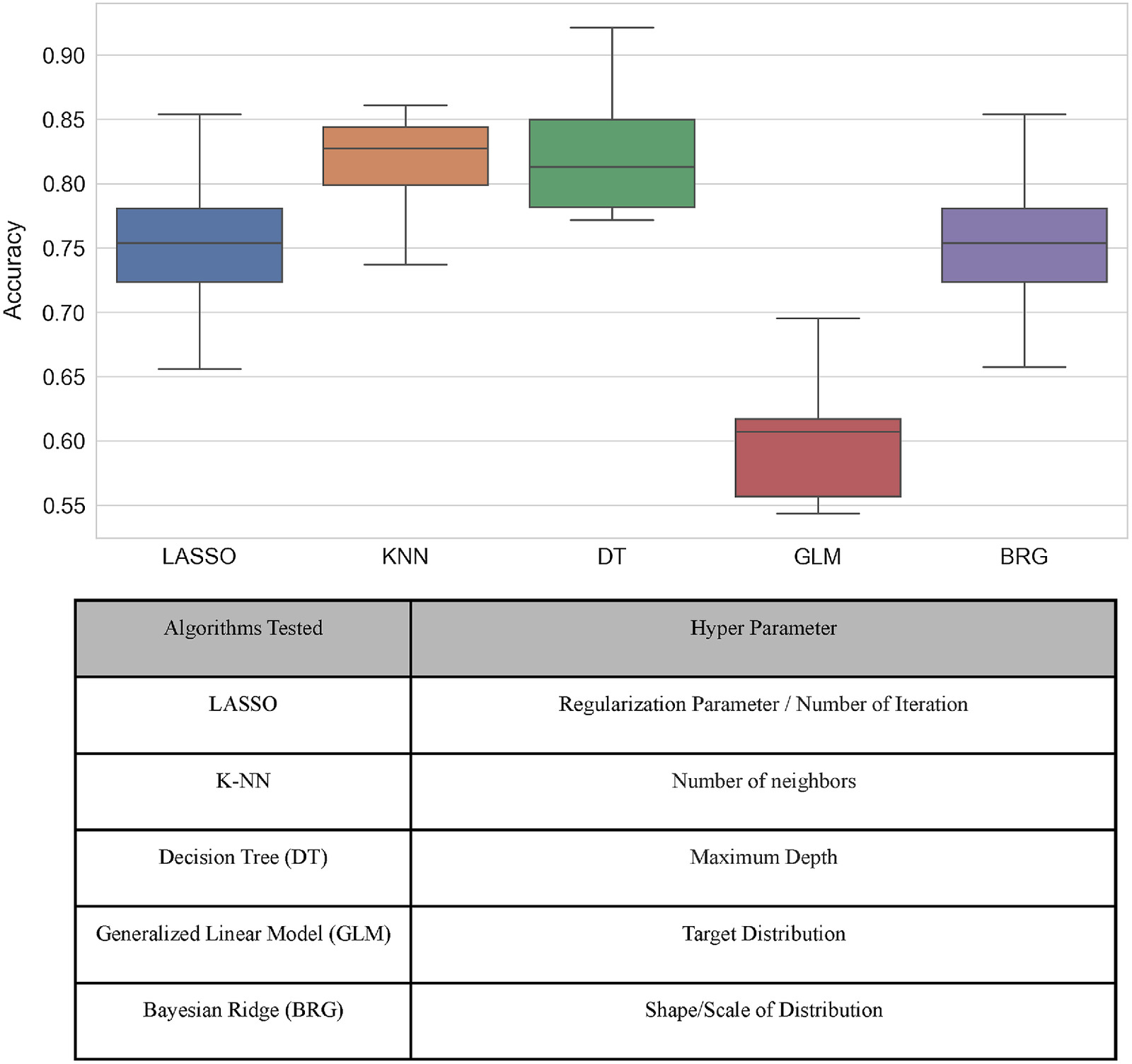
In choosing the best regression model, we examined a set of algorithms in the estimator, which entailed a randomization and splitting of the data set into a training set and validation data set. Ultimately, 70% of the data set was used to train and develop the model, and 15% of the data set was used in the validation and assessment of model fit and reliability. By randomizing the data, we assessed the accuracy of each model with random states of the selection. We also considered different settings of hyperparameters for each algorithm to obtain optimal estimation performance and avoid overfitting. Finally, we assessed the skill of each algorithm against the test data set ( of the data set). The selection process was repeated 1,000 times to obtain a range of accuracy for each algorithm.
Annualized Loss
To validate the study-developed depth–damage functions, aggregate annualized loss was computed and compared with observed historical flood damage within the state of New Jersey. For this, the 2-, 5-, 20-, 100-, 250-, and 500-year pluvial flood hazard layers for 2020 and 2050 were gathered [developed by Bates et al. (2020)]. The maximum inundation depth of each layer was extracted at the geographic location of each Mapbox/Microsoft building footprint within those New Jersey ZCTAs with only pluvial flood risk (no coastal or fluvial risk). The probabilities and associated depths, along with the study-developed depth–damage functions and AVM estimates, were then used to compute the expected annualized loss (AL) for each building in the years 2020 and 2050 [Eq. (3)]. The expected AL in each year is the sum of the probabilities that relate to each flood magnitude multiplied by the damage [Eq. (3)]where and = loss and probability, respectively; and = different return period scenarios. In other words, a loss estimate was computed for a given return period and building by extracting the maximum inundation depth at that building’s footprint and then multiplying the associated damage percent (determined by the depth–damage function) by the building’s AVM. These annualized losses are visually represented by a loss-probability curve, which is represented by the triangular probability distribution formed by the specific probability layers included in this analysis (e.g., Armal et al. 2020) [Fig. 3(b)]. It is important to note an assumption was made that the loss in each probability bin is uniform, which follows guidance from past research (e.g., Armal et al. 2020; Farrow and Scott 2013; Kousky et al. 2013). A statewide pluvial AL value was then computed for both 2020 and 2050 by simply aggregating all building-level AL values that were computed from the hazard layers of each year, respectively. Meanwhile, an observed statewide pluvial flood damage value was computed for each year within the 2004–2018 time period by aggregating the amount paid and observed property damage values from the NFIP and IA claims data sets, respectively. Only NFIP and IA claims tagged to those ZCTAs identified as having only pluvial flood risk were used to compute the observed damage time series. Descriptive statistics were then computed to compare the observed historical statewide pluvial flood damage with the expected AL values for both 2020 and 2050.
(3)
Results
Pluvial Flood Risk
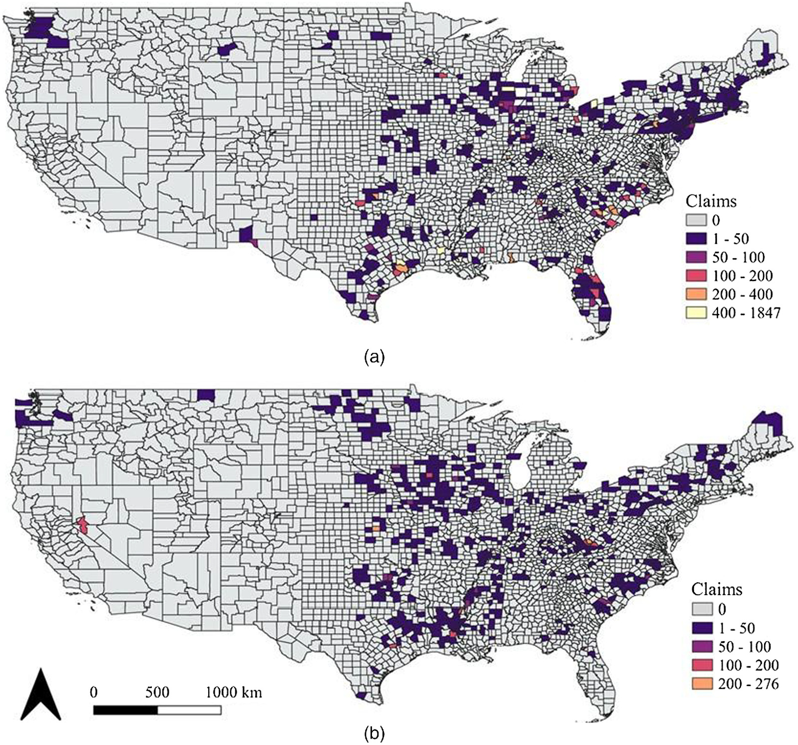
Of the 32,657 ZCTAs located within the contiguous US, we identified 4,766 that have building centroids only exposed to pluvial flood risk (not shown). However, only 3,219 of those ZCTAs have IA claims. Specifically, 2,209 metropolitan and 1,010 nonmetropolitan ZCTAs have claims in the IA database [Figs. 1(a and b), respectively]. Regardless of metropolitan status, most ZCTAs with study-identified pluvial claims are located within the eastern half of the US. In total, we identified 154,809 metropolitan and 13,990 nonmetropolitan pluvial claims within the historical record (2004–2018).
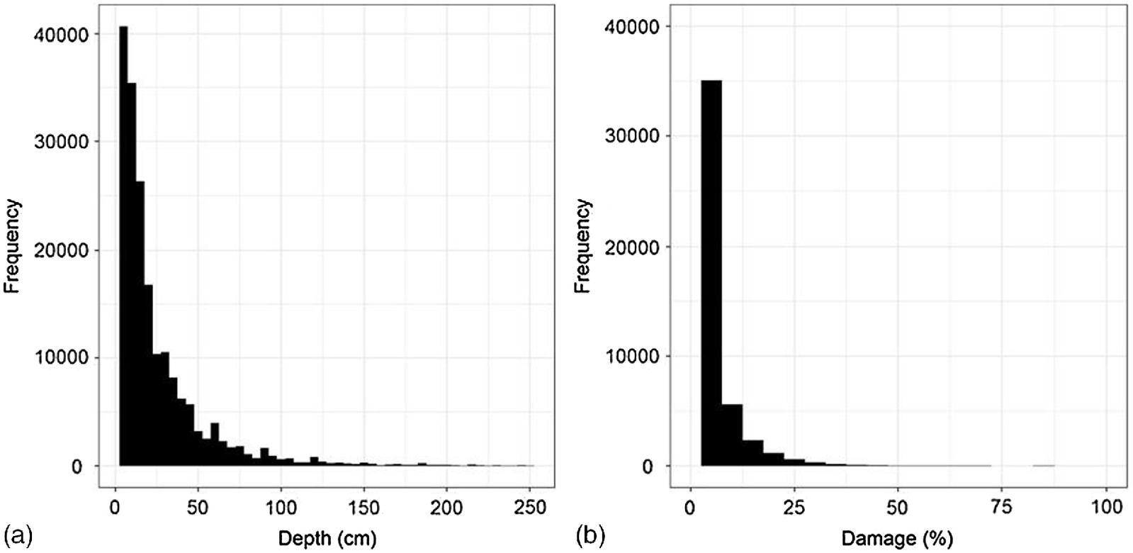
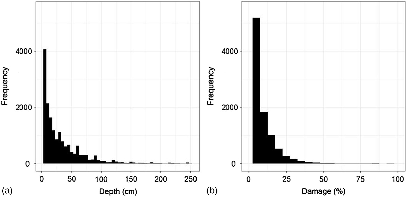
The inundation depths for the metropolitan claims ranged from 2.54 to 251.5 cm, with a median of 15.2 cm, whereas that for the nonmetropolitan claims ranged from 2.54 to 248.9 cm, with a median of 20.3 cm [Table 2 and Figs. 2(a) and 3(a), respectively]. Meanwhile, the distribution of percent damage for the metropolitan claims exhibited a range of 0.5% to 98.8%, with a median percent damage of 1.6% [Table 2 and Fig. 2(b)]. The distribution of percent damage for the nonmetropolitan claims was characterized by a range of 1.0% to 201.2%, with a median percent damage of 3.8% [Table 2 and Fig. 3(b)]. It is important to note that 99% of the depths within the claims data are lower than 195 cm in metropolitan areas and lower than 213 cm in nonmetropolitan areas. The percent damage and inundation depth values exhibited a statistically significant positive relationship for both the metropolitan ( and -value = ) and nonmetropolitan ( and ) claims data sets (not shown).
| Statistical indicator | Metro depths (cm) | Nonmetro depths (cm) | Metro damages (%) | Nonmetro damages (%) |
|---|---|---|---|---|
| Mean | 25.1 | 32.5 | 2.8 | 6.9 |
| Median | 15.2 | 20.3 | 1.6 | 3.8 |
| Q1 | 7.6 | 7.6 | 1.0 | 2.0 |
| Q3 | 30.5 | 45.7 | 2.9 | 8.6 |
| Minimum | 2.54 | 2.54 | 0.5 | 1.0 |
| Maximum | 251.5 | 248.9 | 98.8 | 201.2 |
Note: Included are the mean, median, first quartile (Q1), third quartile (Q3), minimum, and maximum values for each distribution.
Pluvial Depth–Damage Functions
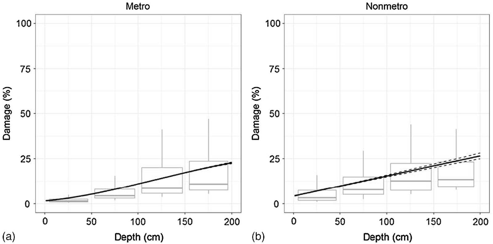
In order to approximate the shape of the damage function curves, a series of regression models were fit to regress the damage percentage on the depth of inundation in both metropolitan and nonmetropolitan contexts. The metropolitan simple linear regression and polynomial regression models were characterized by similar model statistics; however, the coefficient of determination (i.e., ) was slightly greater for the polynomial regression model (Table 2). This indicates that the polynomial model captured a slightly greater amount of the variability in the dependent variable (relative damage) compared with the simple linear regression model (Table 2). Moreover, a partial -test indicated that the polynomial model is a statistical improvement over the simple linear model ( and ).
Similarly, the nonmetropolitan simple linear regression and polynomial regression models were characterized by similar model statistics (Table 3). The coefficient of determination of the polynomial model was slightly greater than that of the simple linear regression model; however, a partial -test indicated that the goodness of fit for the polynomial model was not statistically different from that of the simple linear model ( and ). It is important to note that the residuals plot for both models, and for both the metropolitan and nonmetropolitan data sets, were visually compared and that no meaningful differences were observed (not shown).
| Model type | RMSE | MAE | |
|---|---|---|---|
| SLR-metro | 0.21 | 3.4 | 1.9 |
| POLY-metro | 0.23 | 3.5 | 1.9 |
| SLR-nonmetro | 0.13 | 7.7 | 5.0 |
| POLY-nonmetro | 0.14 | 7.7 | 5.0 |
Note: Statistics include the coefficient of determination (), root-mean squared error (RMSE), and mean absolute error (MAE). All models are characterized by statistical significance ().
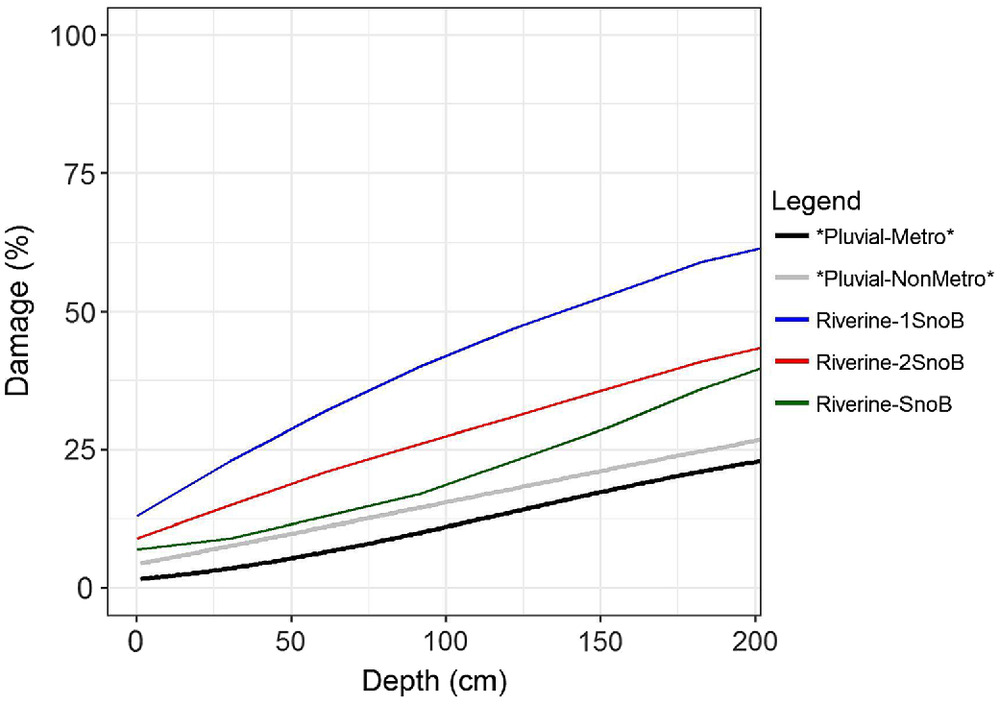
For consistency, we decided to select the polynomial regression model to predict relative damage using depth of inundation for the metropolitan and nonmetropolitan data sets [Figs. 4(a and b), respectively]. As a result, for each context, the damage functions are represented by second-polynomial functions in order to allow for the prediction of damage for depths ranging from 1 to 200 cm. The curves derived from this modeling application are hereafter referred to as the metropolitan and nonmetropolitan depth–damage functions.
New Jersey Case Study
As discussed previously, to develop an expectation of property value, our AVM approach was implemented on a sample data set of 600,000 properties in New Jersey. The results indicated that decision tree (DT) and -nearest neighbors (K-NN) regularly outperformed other algorithms, with median accuracy of around 0.82 (Fig. 5). Ultimately, we selected the DT regressor as the main algorithm in the estimator because that algorithm requires less execution time, convergence time, and memory usage compared with K-NN.
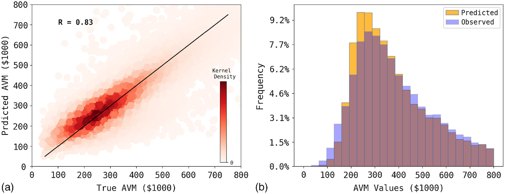
Next, we evaluated the skill of the model by removing known AVM and market values in 30% of properties and running the estimator to fill the gaps. The results showed a high correlation between the simulated AVM values and actual AVM values [Fig. 6(a)]. Furthermore, the model replicated the distribution of observed AVM values in the simulated results. However, the outcome of the model slightly underestimated the observed values, particularly toward the extremes [Fig. 6(b)].
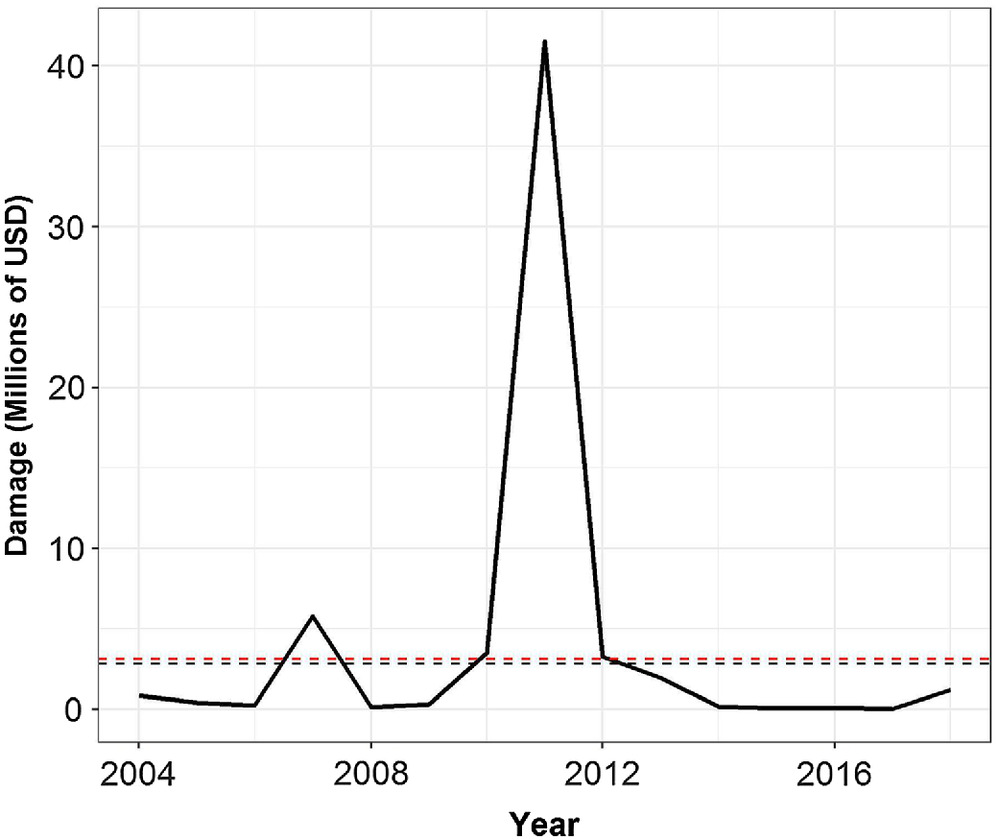
Next, the depth–damage functions were applied to buildings located within pluvial only ZCTAs within the state of New Jersey using the depths associated with the pluvial hazard layers and the AVMs developed here. The aggregate annualized loss across the pluvial-only ZCTAs within the state is 2.7 million USD in 2020, and 3.1 million USD in 2050 (Fig. 7). In comparison, we identified 102 of the 595 ZCTAs within the state of New Jersey exposed to only pluvial flooding. A total of 14,933 IA and 1,664 NFIP claims were tagged to the 102 pluvial ZCTAs within New Jersey during the 2004–2018 time period. The average statewide damage (pluvial only ZCTAs) during that period was 3.96 million USD (Fig. 7). Notably, pluvial flooding caused 41.5 million USD worth of damage in 2011, most of which can be attributed to rainfall associated with Hurricane Irene.
Discussion and Conclusions
The primary objective of this study was to develop pluvial depth–damage functions using existing historical insurance/damage payout data. Within this study, building-level complexity for the damage functions could not be produced due to the lack of adequate property-level differentiation. However, it was found that reliable differentiation does exist between metropolitan and nonmetropolitan contexts. For both the metropolitan and claims data sets, a polynomial regression model was selected over a simple linear model to characterize the depth–damage function. The metropolitan polynomial model explained 23% of the variance. This is in line with the results of the multivariate models developed by Van Ootegem et al. (2015), which explained 18% and 28%. Although Van Ootegem et al. (2015) used multiple predictors within their models, the similar results of the simpler metropolitan model developed here may be explained by the role of flood depth as the most important predictor of damage. In contrast, the nonmetropolitan model developed here explained 14% of the damage variance, which is less than that of the models developed by Van Ootegem et al. (2015). This difference may be because the Van Ootegem et al. (2015) damage models were developed using a survey data set from an urban environment.
A secondary objective of this study was to test the utility of the developed depth–damage functions. Because the functions developed here are relative (in percent form), an AVM was developed to obtain an economic value for each property within the state of New Jersey. The building values of those properties were estimated as the replacement cost of structure on the property. These were then combined with pluvial-only flood hazard layers and the derived depth–damage functions to compute an annualized loss estimate for the portion of economic risk in New Jersey resulting from expected pluvial flooding on an annual basis. It is clear that the pluvial damage functions deviated significantly from the damage function in the HAZUS framework, which reflect coastal and riverine damage based on observations related to water depth in prior USACE studies (Fig. 8). Additionally, a comparison of the expected flood economic damage in both 2020 and 2050 aligned with the observed payouts during the 2004–2018 time period (when accounting for the higher average over the period due to the anomaly of high payouts in 2011) (Fig. 7).
Further research is needed to refine the pluvial depth–damage functions developed here. However, our results prove that the depth–damage relationship for pluvial flooding is likely to be different from that for other flood types (e.g., fluvial). This was illustrated by our New Jersey case study. Additionally, although the norm is to apply riverine and coastal damage functions, these do not capture the full expectation of annualized economic loss. Although New Jersey is situated along the coast, about half of the properties at risk of flooding within the current environmental context are at risk of pluvial-only hazards. Although pluvial-only hazards are not as economically damaging as coastal and riverine flood hazards, they tend to affect a larger proportion of properties in the US. As such, the economic impacts of these hazards cannot be ignored. Future research on the economic risk associated with flooding will benefit from the inclusion of pluvial flood risk.
Data Availability Statement
Some or all data, models, or code that support the findings of this study are available from the corresponding author upon reasonable request. Table 1 contains a list of all data used in the analysis. All of those data are available for sharing with the exception of FSF hazard layers, Lightbox Parcel Data, and the County Assessor Data, which are bound by proprietary restrictions.
Acknowledgments
The authors would like to thank the comments from the blind peer reviewers and editors of this paper. Both provided valuable feedback that has been integrated into the final version of the paper.
References
Armal, S., J. R. Porter, B. Lingle, Z. Chu, M. L. Marston, and O. E. Wing. 2020. “Assessing property level economic impacts of climate in the us, new insights and evidence from a comprehensive flood risk assessment tool.” Climate 8 (10): 116. https://doi.org/10.3390/cli8100116.
Bates, P. D., et al. 2020. “Combined modelling of US fluvial, pluvial and coastal flood hazard under current and future climates.” Water Resour. Res. 57 (2): 1–29. https://doi.org/10.1029/2020WR028673.
Blake, E. S., and D. A. Zelinsky. 2018. National Hurricane Center tropical cyclone report: Hurricane Harvey, 76. Miami: NH Center.
Borchani, H., G. Varando, C. Bielza, and P. Larrañaga. 2015. “A survey on multi-output regression.” Wiley Interdiscip. Rev.: Data Min. Knowl. Discovery 5: 216–233. https://doi.org/10.1002/widm.1157.
Butler, M. A., and C. L. Beale. 1994. Rural-urban continuum codes for metro and nonmetro counties, 1993. Washington, DC: Economic Research Service.
Cutter, S. L., C. T. Emrich, M. Gall, and R. Reeves. 2018. “Flash flood risk and the paradox of urban development.” Nat. Hazard. Rev. 19 (1): 05017005. https://doi.org/10.1061/(ASCE)NH.1527-6996.0000268.
Farrow, S., and M. Scott. 2013. “Comparing multistate expected damages, option price and cumulative prospect measures for valuing flood protection.” Water Resour. Res. 49 (5): 2638–2648. https://doi.org/10.1002/wrcr.20217.
FEMA. 2020a. “Individual assistance claims database.” Accessed May 20, 2020. https://www.fema.gov/openfema-data-page/individual-assistance-housing-registrants-large-disasters-v1.
FEMA. 2020b. “National flood insurance program database.” Accessed May 20, 2020. https://www.fema.gov/openfema-data-page/fima-nfip-redacted-claims.
First Street Foundation. 2020. “FSF flood hazard layers.” Accessed June 12, 2020. https://firststreet.org/api/.
Freni, G., G. La Loggia, and V. Notaro. 2010. “Uncertainty in urban flood damage assessment due to urban drainage modeling and depth-damage curve estimation.” Water Sci. Technol. 61 (12): 2979–2993. https://doi.org/10.2166/wst.2010.177.
Hayhoe, K., D. J. Wuebbles, D. R. Easterling, D. W. Fahey, S. Doherty, J. Kossin, W. Sweet, R. Vose, and M. Wehner. 2018. “Our changing climate.” In Impacts, risks, and adaptation in the United States: Fourth national climate assessment, volume II, Edited by D. R. Reidmiller, C. W. Avery, D. R. Easterling, K. E. Kunkel, K. L. M. Lewis, T. K. Maycock, and B. C. Stewart, 72–144. Washington, DC: US Global Change Research Program.
Kaspersen, P. S., N. H. Ravn, K. Arnbjerg-Nielsen, H. Madsen, and M. Drews. 2015. “Influence of urban land cover changes and climate change for the exposure of European cities to flooding during high-intensity precipitation.” Proc. Int. Assoc. Hydrol. Sci. 370 (Jan): 21–27. https://doi.org/10.5194/piahs-370-21-2015.
Kellens, W., W. Vanneuville, E. Verfaillie, E. Meire, P. Deckers, and P. De Maeyer. 2013. “Flood risk management in Flanders: Past developments and future challenges.” Water Resour. Manage. 27 (10): 3585–3606. https://doi.org/10.1007/s11269-013-0366-4.
Kousky, C., E. O. Michel-Kerjan, and P. A. Raschky. 2018. “Does federal disaster assistance crowd out flood insurance?” J. Environ. Econ. Manage. 87 (Jan): 150–164. https://doi.org/10.1016/j.jeem.2017.05.010.
Kousky, C., M. Walls, and Z. Chu. 2013. Flooding and resilience: Valuing conservation Investments in a world with climate change. Washington, DC: Economic Research Service.
Lightbox. 2019a. “Digital map parcel boundaries.” Accessed October 2, 2019. https://www.digmap.com/solutions/building-land-development/.
Lightbox. 2019b. “Property and building characteristics database. DMP (digital map products) Lightbox dataset.” Accessed October 2, 2019. https://www.digmap.com/solutions/building-land-development/.
Mastelini, S. M., V. G. T. da Costa, E. J. Santana, F. K. Nakano, R. C. Guido, R. Cerri, and S. Barbon. 2019. “Multi-output tree chaining: An interpretative modelling and lightweight multi-target approach.” J. Signal Process. Syst. 91 (2): 191–215. https://doi.org/10.1007/s11265-018-1376-5.
McAlpine, S. A., and J. R. Porter. 2018. “Estimating recent local impacts of sea-level rise on current real-estate losses: A housing market case study in Miami-Dade, Florida.” Popul. Res. Policy Rev. 37 (6): 871–895. https://doi.org/10.1007/s11113-018-9473-5.
Microsoft. 2018. “Satellite derived building footprint layers.” Accessed April 4, 2020. https://github.com/Microsoft/USBuildingFootprints.
National Academies of Sciences, Engineering, and Medicine. 2019. Framing the challenge of urban flooding in the United States. Washington, DC: National Academies Press. https://doi.org/10.17226/25381.
NOAA (National Oceanic and Atmospheric Administration). 2020. “SLOSH model inundation GIS layers.” Accessed June 12, 2020. https://slosh.nws.noaa.gov/sloshPriv/meow.php.
Olsen, A. S., Q. Zhou, J. J. Linde, and K. Arnbjerg-Nielsen. 2015. “Comparing methods of calculating expected annual damage in urban pluvial flood risk assessments.” Water 7 (12): 255–270. https://doi.org/10.3390/w7010255.
Rosenzweig, B. R., L. McPhillips, H. Chang, C. Cheng, C. Welty, M. Matsler, D. Iwaniec, and C. I. Davidson. 2018. “Pluvial flood risk and opportunities for resilience.” Wiley Interdiscip. Rev.: Water 5 (6): e1302.
Rözer, V., H. Kreibich, K. Schröter, M. Müller, N. Sairam, J. Doss-Gollin, U. Lall, and B. Merz. 2019. “Probabilistic models significantly reduce uncertainty in Hurricane Harvey pluvial flood loss estimates.” Earth’s Future 7 (4): 384–394. https://doi.org/10.1029/2018EF001074.
Smith, A. B. 2020. “NOAA national centers for environmental information. Dataset.” Accessed June 8, 2020. https://www.ncdc.noaa.gov/billions/.
ten Veldhuis, J. A. E. 2011. “How the choice of flood damage metrics influences urban flood risk assessment.” J. Flood Risk Manage. 4 (4): 281–287. https://doi.org/10.1111/j.1753-318X.2011.01112.x.
USACE. 2019. “National structures database.” Accessed October 5, 2019. https://github.com/HydrologicEngineeringCenter/NSI.
USDA. 2020. “Rural-urban continuum codes (Beale codes).” Accessed June 10, 2020. https://www.ers.usda.gov/data-products/rural-urban-continuum-codes.aspx.
Van Ootegem, L., E. Verhofstadt, K. Van Herck, and T. Creten. 2015. “Multivariate pluvial flood damage models.” Environ. Impact Assess. Rev. 54 (Sep): 91–100. https://doi.org/10.1016/j.eiar.2015.05.005.
Viterbo, F., K. Mahoney, L. Read, F. Salas, B. Bates, J. Elliott, B. Cosgrove, A. Dugger, D. Gochis, and R. Cifelli. 2020. “A multiscale, hydrometeorological forecast evaluation of national water model forecasts of the May 2018 Ellicott City, Maryland, flood.” J. Hydrometeorol. 21 (3): 475–499. https://doi.org/10.1175/JHM-D-19-0125.1.
Wing, O. E., P. D. Bates, A. M. Smith, C. C. Sampson, K. A. Johnson, J. Fargione, and P. Morefield. 2018. “Estimates of present and future flood risk in the conterminous United States.” Environ. Res. Lett. 13 (3): 034023. https://doi.org/10.1088/1748-9326/aaac65.
Zachry, B. C., W. J. Booth, J. R. Rhome, and T. M. Sharon. 2015. “A national view of storm surge risk and inundation.” Weather Clim. Soc. 7 (2): 109–117. https://doi.org/10.1175/WCAS-D-14-00049.1.
Zhou, Q., P. S. Mikkelsen, K. Halsnæs, and K. Arnbjerg-Nielsen. 2012. “Framework for economic pluvial flood risk assessment considering climate change effects and adaptation benefits.” J. Hydrol. 414 (Jan): 539–549. https://doi.org/10.1016/j.jhydrol.2011.11.031.
Information & Authors
Information
Published In

Natural Hazards Review
Volume 24 • Issue 1 • February 2023
Copyright
This work is made available under the terms of the Creative Commons Attribution 4.0 International license, https://creativecommons.org/licenses/by/4.0/.
History
Received: Oct 21, 2021
Accepted: Sep 26, 2022
Published online: Dec 15, 2022
Published in print: Feb 1, 2023
Discussion open until: May 15, 2023
Authors
Metrics & Citations
Metrics
Citations
Download citation
If you have the appropriate software installed, you can download article citation data to the citation manager of your choice. Simply select your manager software from the list below and click Download.