Characterization of the Water Supply of the Rio Grande Project Based on Rio Grande Compact Reports 1940–2020
Publication: Journal of Water Resources Planning and Management
Volume 150, Issue 4
Abstract
The focus of this study is the 1938 Rio Grande Compact water supply. The compact is an interstate agreement signed in 1938 between the states of Colorado, New Mexico, and Texas to evenly apportion the waters of the Rio Grande Basin. A shortage in deliveries is at the center of a lawsuit that began in 2011, went to the Supreme Court in 2013, and has not been resolved. This research statistically characterized the differences between water available and water delivered by Colorado and New Mexico, signatories of the Rio Grande Compact with Texas, to understand changes over time and uncover potential autocorrelations. Unexpected changes in water deliveries can have serious financial impacts on communities, thus the importance of shedding light into the behavior of the differences between water available and delivered. One of the findings of the research was that the annual credit/debit time series for Colorado was significantly correlated with the current and immediately previous scheduled delivery as well as with itself in the two previous years, and the behavior is explained by a transfer function model (TFM). For New Mexico, the annual credit/debit series did not display a clear pattern; therefore, it was not possible to characterize its relationship with scheduled delivery with the method examined. This technical note contributes to the extensive body of literature of the Rio Grande Compact in a way no other study has done as well as contributing to the wealth of literature related to the use of the transfer function model in hydrology. The main contribution of the study is the methodology developed and used, which could be useful to other river systems and transboundary water sharing agreements.
Practical Applications
This research statistically characterized the differences between water available and water delivered, also known as credits and debits, by Colorado and New Mexico, signatories of the Rio Grande Compact with Texas, to understand changes over time and uncover potential autocorrelations. A legal conflict between the signatories of the compact has lasted over a decade. Texas alleges that New Mexico is extracting groundwater, shortening their share of the water. Unexpected changes in water deliveries can have serious financial impacts on communities so shedding light on the differences between water available and water delivered can contribute to the debate. One of the research findings was that the annual credit/debit time series for Colorado was significantly correlated with the current and immediately previous scheduled delivery as well as with itself in the two previous years, and the behavior is explained by a TFM. For New Mexico, the annual credit/debit series did not display a clear pattern; therefore, it was not possible to characterize its relationship with scheduled delivery with the method examined. The main contribution of the study is the methodology developed and used, specifically the TFM, which could be tweaked to fit other river systems and transboundary water sharing agreements.
Introduction
Water sharing agreements between upstream and downstream entities are customary in many countries in the world. Issues arise when present obligations are based on hydrological conditions of the past that no longer represent the present. That has, and continues to be, the cause of disagreement and disputes between parties.
The focus of this study is the 1938 Rio Grande Compact (the Compact) water supply; however, to study it, one must learn its history as well as that of the Rio Grande Project (RGP). Fig. S1 shows the map of the geographical location encompassed by the Rio Grande Compact.
In response to claims by Mexico in 1890s of the US overdiverting water and increasing shortages in the neighboring country (American Journal of International Law 1907; Shupe et al. 1989; King and Maitland 2003), the US Department of the Interior began researching ways by which the water from the Rio Grande could be better managed (Littlefield 1999). An act of Congress in 1905 approving the construction and operation of a project called the RGP (Autobee 1994) was the result of research and a proposal from the US Bureau of Reclamation to build a dam where the current Elephant Butte Reservoir is located.
The project delivers water to two irrigation districts, one in Texas and one in New Mexico, in addition to helping fulfill the requirements of the 1906 treaty with Mexico (Littlefield 1999). The storage capacity of Elephant Butte Reservoir, about 2 million acre-feet (MAF) (about ) buffers wide swings in Rio Grande water supply from upstream to provide a more reliable water supply for the RGP downstream. Caballo Dam, built later, is intended to provide additional regulating and flood control capability.
The Compact is an interstate agreement signed in 1938 between the states of Colorado, New Mexico, and Texas to evenly apportion the waters of the Rio Grande Basin. The Compact was ratified by the states in 1938, and by Congress in 1939, to settle disputes going back to the late 1800s (Hill 1974). A paramount purpose of the Compact was, and continues to be, to safeguard the RGP and its operations under the conditions that existed at the time the Compact was signed (Rio Grande Compact Commission 1939, p. 5, 2020).
Over the years, the three signatory states of the Compact have had disagreements (Mix et al. 2012) and from time to time sued each other, but the disagreements have been resolved. However, the current conflict began in 2011 when New Mexico sued the federal government and the two irrigation districts in the US that are part of the RGP, alleging that an agreement made in 2008 between the US Bureau of Reclamation and the RGP districts was shortcutting New Mexico of the water to which the Compact gave it a right. In 2013, Texas took the case to the Supreme Court, accusing New Mexico farmers and cities below Elephant Butte Reservoir of extracting groundwater to their detriment, thus shortening their share of the water. Given that the Rio Grande is the main water supply of the RGP and the shortage in deliveries is at the center of the current court case, this study characterized the relationship between Compact obligations and actual deliveries by doing a statistical examination of the Rio Grande Compact operations and accounting from 1940 to 2020. The authors used annual reports issued by the Compact Commission to describe the patterns of credits and debits relative to the available water supply between 1940 and 2020 to estimate when Colorado and New Mexico are more likely to have a credit or a debit.
This technical note contributes to the extensive body of literature of the Rio Grande Compact in a way that no other study has done, specifically by characterizing debits and credits for Colorado and for New Mexico. In 1974, Reynolds and Mutz (1974) studied water deliveries under the Rio Grande Compact. They plotted the deliveries of Colorado and New Mexico but did not statistically characterize the credits or debits. They pointed out something that was confirmed with this technical note, which is that the release from project storage was less than 790,000 acre-feet a year for all but 4 of the 33 years since the ratification of the Compact and that New Mexico and Colorado were in debit status most of that time. In 2011, Sandoval-Solis and McKinney (2011) conducted a risk analysis of the 1944 treaty between the United States and Mexico for the Rio Grande/Rio Bravo Basin. They contrasted the expected treaty obligations with actual historic performance and used measures of reliability, resilience, and vulnerability for their analysis. The topic and approach of their study is like this technical note in the sense that it is also an attempt to characterize differences between the expected and the actual to enlighten the path ahead. They concluded that under drought conditions, the system was not able to recover as expected, just like the one under the Rio Grande Compact, and that the deficits were bigger than what was estimated resulting in increased difficulties for signatories of the treaty as well as beneficiaries of the water agreement in both countries. In 2012, Mix et al. (2012) characterized the changes in streamflow at Lobatos gauge in Colorado to determine whether they were statistically significant between periods, but did not characterize the behavior of credits and debits of Colorado or New Mexico like this technical note does. They also conducted a water balance accounting to reveal volumetric changes to identify when those require attention. Besides the references mentioned, the authors did not find other published work that has statistically characterized the pattern of credits and debits for Colorado and New Mexico under the Rio Grande Compact of 1938, or other rivers in the US.
Data and Variables
The data come from the reports of the Rio Grande Compact Commission from 1940 to 2020, specifically the tables called “Deliveries by Colorado at State Line” and “Deliveries by New Mexico at Elephant Butte.” The tables have monthly data for New Mexico and Colorado for index supply, scheduled delivery, actual delivery, and annual and cumulated credits and debits for each year. Table S1 documents these data.
The index supply is defined for Colorado and New Mexico in Articles III and IV of the Compact, respectively. In the case of Colorado, the index supply is composed of the flow measurements of two index supplies, Conejos and Rio Grande. For New Mexico, the index supply is the flow record of the Rio Grande measured at one gauging station, Otowi (Garrick et al. 2018).
The second variable is scheduled delivery. It defines the quantities of water, via a linear relationship, that each state would be responsible for delivering to the designated point of the downstream counterpart given the index supply for that year (Articles III and IV of the Compact).
The third variable is actual delivery. Colorado’s actual delivery to New Mexico takes place at the Lobatos gauge near the Colorado–New Mexico state line, and differences between the index supply and the actual supply are accounted for as an annual credit or debit to Colorado. New Mexico originally delivered water to Texas at the San Marcial gauge on the Rio Grande, upstream of Elephant Butte Reservoir. The delivery point for Compact accounting purposes was moved to Elephant Butte Dam, effective January 1, 1949 (Rio Grande Compact Report 1939; Garrick et al. 2018).
Data Description
To summarize the hydrologic history, scheduled delivery data sets for Colorado and New Mexico were considered because they are directly related to the upstream flows and with the supply of water (Fig. 1). Outlier data points in years 1941 and 1942 come from the overdelivery by New Mexico of 108.3 thousand acre-feet (KAF) () in 1941 and the spill in 1942 due to floods (Reynolds and Mutz 1974; Rio Grande Compact Reports 1939).
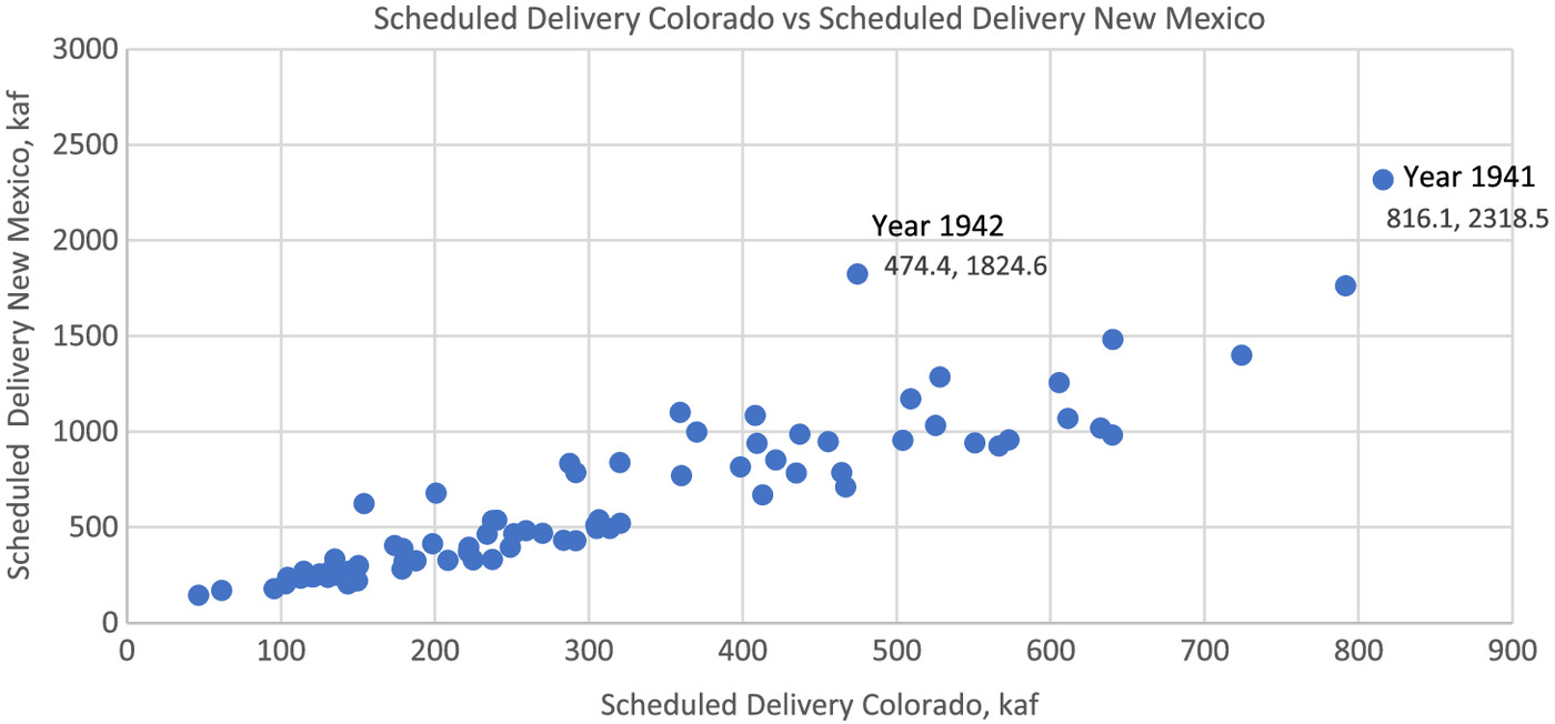
The correlation coefficient between scheduled delivery for Colorado and for New Mexico for the entire period of record was 0.93, implying, as expected, a strong positive linear relationship between scheduled deliveries of Colorado and New Mexico. The hydrologic explanation is that the index gauge flows are driven by the same climatic conditions as the delivery gauge flow.
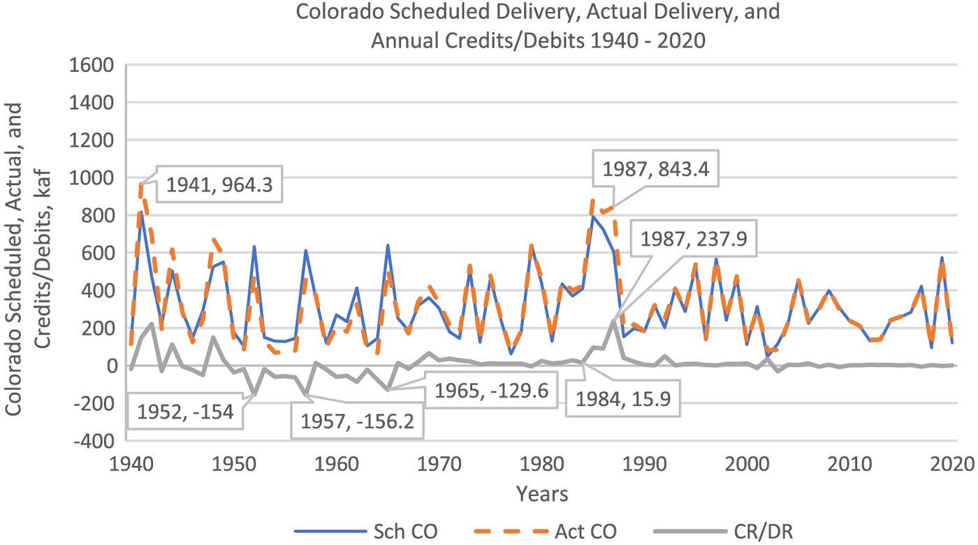
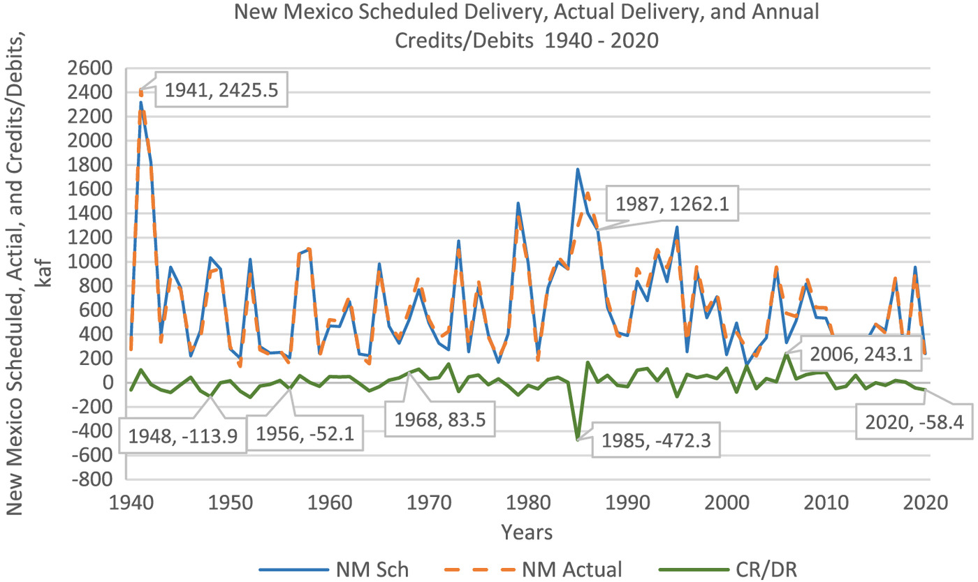
The dynamics of the scheduled delivery and actual delivery, and their difference, the annual credits or debits for each of the states, can be seen in Figs. 2 and 3 and in Table 1, which summarizes the means and standard deviations.
| Series | Colorado | New Mexico |
|---|---|---|
| Scheduled delivery | ||
| Actual delivery | ||
| Credits and debits |
For Colorado, the mean values for scheduled delivery, actual delivery, and credits and debits were 309, 315, and 5.90; and standard deviations were 184, 208, and 61, respectively. For New Mexico, the mean values for scheduled delivery, actual delivery, and credits and debits were 636, 644, and 8.25; and standard deviations were 429, 421, and 87, respectively. This means that while the scheduled delivery set forth in Articles III and IV (Rio Grande Compact Commission 1939) is defined to 1.4 MAF of water for Colorado and 2.3 MAF for New Mexico, most of the time the system has found itself in the lower end of the schedule, particularly in recent years.
Credits and Debits for Colorado and New Mexico
From here forward, all references of credits and debits in this document refer to annual credits and debits except when stated that they are accrued.
Colorado
Contrasting the credit/debit time series with the annual and accrued thresholds established for Colorado in Article VI (Rio Grande Compact Commission 1939) (Fig. 4), Colorado has gone over the annual debit threshold of 100 KAF () in 1957 and 1965; and the accrued threshold of 150 KAF () between 1952 and 1984. Between 1940 and 1949, Colorado had almost the same number of years with annual debits as with credits. Between 1950 and 1967, there are mainly debits, except for 1958 and 1966. From 1968 to 2020, there are all credits, except for the years of 2001 and 2003 when Colorado incurred in a debit higher than 10 KAF ().
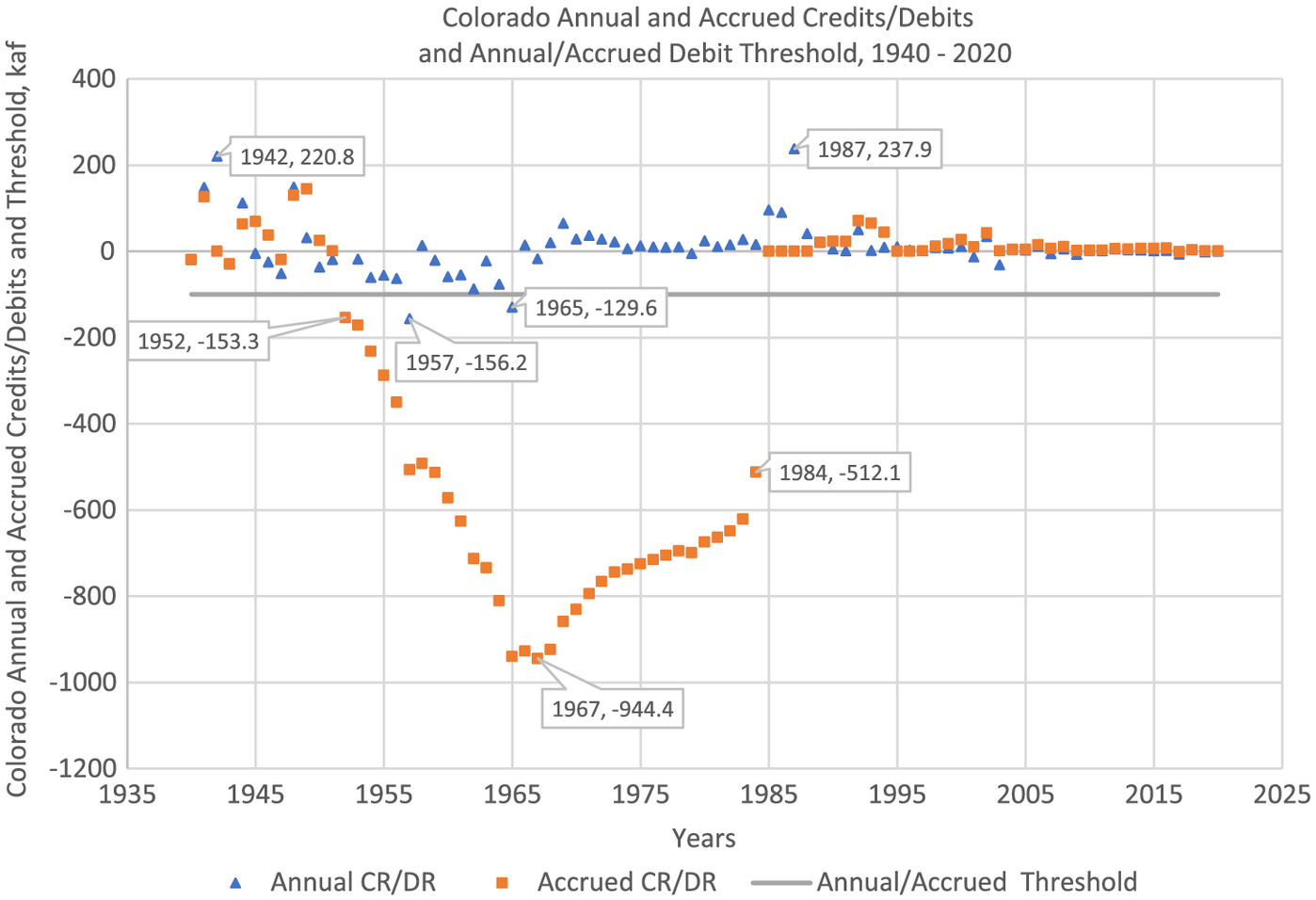
The potential reason why Colorado’s credits and debits have mostly balanced since 1968 is because in 1966 Texas and New Mexico filed suit against Colorado in the US Supreme Court for an alleged violation of the Compact obligations (Shupe et al. 1989). The complaint cited the amount of accrued debit of Colorado, which was over 900 KAF (), and urged Colorado to speed up the analysis and implementation of the plan to salvage water from the Closed Basin Division of the San Luis Valley Project to the Rio Grande for delivery to New Mexico and Texas (Whipple and López 2005). In 1968, the US Supreme Court granted a continuance requested by the three states [Texas v. Colorado, 391 U.S. 901, 88 S. Ct. 1649, 20 L.Ed.2d 416 (1968)]. In keeping with the agreed stipulations of the continuance, Colorado instituted water rights priority administration in its portion of the Rio Grande Basin; the Bureau of Reclamation implemented the Closed Basin Division (Mix et al. 2012); and through 1984, Colorado met the obligations of the continuance and the condition to report frequently (Whipple and López 2005). The spill of 1985 canceled all the accrued debits of Colorado and New Mexico, and by court order (474 U.S. 1017 of 1985) the motion for dismissal without prejudice of the original 1966 suit was granted (Shupe et al. 1989; McKusick 1994).
New Mexico
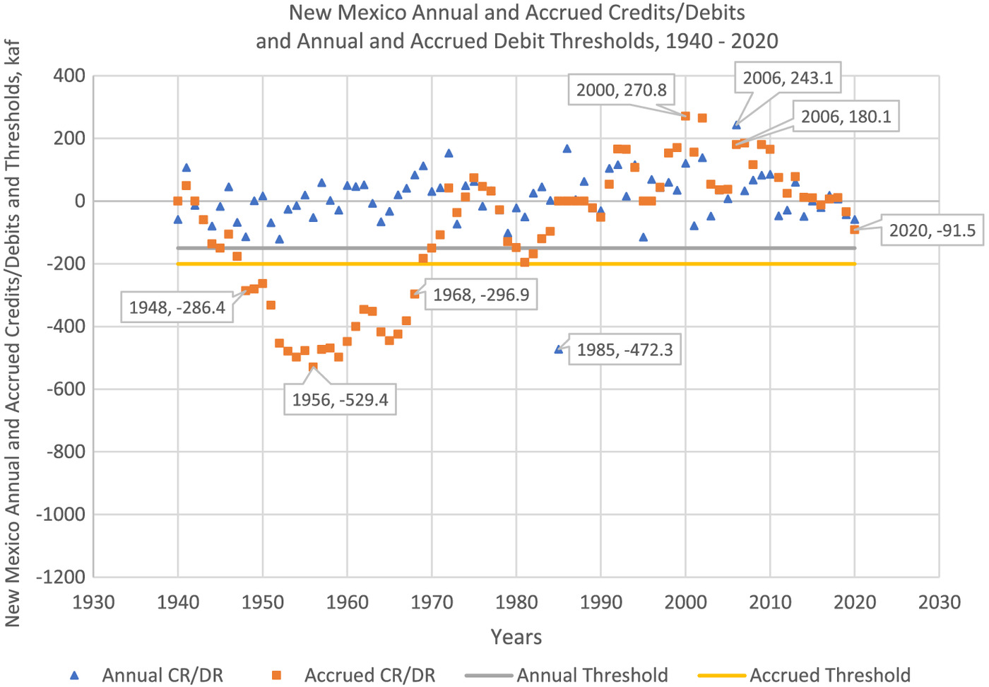
Contrasting the credit/debit time series with the annual and accrued thresholds established for New Mexico in Article VI (Rio Grande Compact Commission 1939), Fig. 5 details that New Mexico exceeded the accrued threshold of 200 KAF () between 1948 and 1968. Between 1940 and 1950, New Mexico had three years of credits (1941, 1946, and 1950) and one year (1949) close to a balance, with a credit of 1.2 KAF (). The rest of the years are debits ranging from () in 1942 to () in 1948. Between 1951 and 1978, there were almost twice as many debits as there were credits; however, between 1979 and 2001, and 2002 and 2020, the opposite is true, there are almost twice as many credits as there are debits. In the early years the credits and debits of Colorado and New Mexico did not have a discernible pattern, but both mainly incurred debits. After 1985 that changed for both.
Methods
The study considered the entire period of record for both series, credits and debits, and then introduced qualifiers to make distinctions between hydrological conditions of an uncertain and changing environment (NMBGMR 2022). The conditions were called high (H) and low (Lo), early (E) and late (La). The (H) and (Lo) resulted from plotting a cumulative distribution for scheduled delivery for each state (SchDCO and SchDNM) to determine when natural breaks in the distribution occurred, reflecting wet periods and drought periods. The (E) and (La) indicate the period before and after the spill that occurred in 1985 (Rio Grande Compact Report 1939), which coincides with long-term conditions of the region toward a more arid climate (NMBGMR 2022). With the entire period of record and the four qualifiers, the authors calculated descriptive statistics for all the series, visualized the distribution of the series and their relationships, and conducted correlation analyses. The purpose of using the four qualifiers was to capture differences between specific hydrologic conditions of the flows and not necessarily of the system. In turn, the point of using a statistical approach is to focus on index and delivery flows to avoid the infinite complexity in the hydrology of the system.
A time series model using the autoregressive integrated moving average (ARIMA) process was performed to understand the temporal characteristics of each series of credit/debit for Colorado and New Mexico. The ARIMA model can be denoted ARIMA , where is the order of an autoregressive model, is the degree of differencing, and is the order of the moving average model. The authors then fitted the transfer function model (TFM) to identify hydrologic factors that determine patterns of credit/debit series. The TFM combines two approaches, time series with causal, to estimate the output series from past values of more than one interconnected input time series (Hasanah et al. 2013). This study used a TFM with annual credit/debit as the output series () and scheduled delivery as the input series (). For more details, refer to Supplemental Materials. Once the models that fit the input and output series were identified, the second step was to do prewhitening for both series. Prewhitening uses ARIMA models for the input series and consists of “transformation processes which are correlated to the behavior of white noise which are not correlated” (Hasanah et al. 2013, p. 319). The prewhitening process detects the cross correlation between the input and output series using the plot.
The model selection was primarily based on the Akaike information criterion (AIC), which is a mathematical method for evaluating how well a model fits the data from which it was generated. The model with the smallest AIC value was chosen as the best model. The root-mean-square error (RMSE) and the mean absolute percentage error (MAPE) were considered to determine which model was most accurate in prediction. For details, refer to Supplemental Materials. All statistical analyses were conducted using the software R (version 4.1.0).
This technical note contributes to build the broad body of literature regarding how transfer function models have been used to date in the field of hydrology because none of the publications reviewed used a transfer function model to describe the future prediction value of the annual credit/debit time series (output series or ) based on the past values from one or more interconnected time series (input series or scheduled delivery and previous year credit/debit). One documented use of TFM was in 1985 by Maidment et al. (1985), when the model was used to represent the relationship between daily rainfall and urban water use. TFM has also been used in regionalization at the finer scale for snow interception, infiltration root zone, surface runoff evapotranspiration, slow and fast interflow, baseflow, routing, and potential evapotranspiration (Samaniego et al. 2010). TFM has helped estimate travel time of recharge water through the deep vadose zone by describing the relationship between the variation in rainfall and evapotranspiration, and the changes in the level of the groundwater table (Mattern and Vanclooster 2010). In turn, Labat and Mangin (2015) applied the TFM to trace the flow of a contaminant via a tracer test in karstic systems. Also in 2015, Baillieux et al. (2015) used the TFM in the study of the evolution of groundwater quality at aquifer outlets by considering historical land use in the area under study. In the paper they document five studies that used TFM in research related to groundwater quality at an aquifer outlet. Continuing with the groundwater topic, Jimenez-Martinez et al. (2016) derived a TFM between effective rainfall and groundwater levels to predict groundwater levels for rainfall for high, medium, and low emissions scenarios from climate projections for the United Kingdom. TFM was used by Pezij et al. (2020) to characterize soil moisture dynamics, which they stated was the first time TFM was used for that purpose, with precipitation and evapotranspiration as inputs. In their paper they provide a literature reference related to the use of TFM in hydrological applications from 1980 to 2014. A study conducted by Jeong et al. (2018) used TFM for estimating water table fluctuations of unsaturated infiltration fluxes at two monitoring locations. Other examples of the use of TFM in hydrology include a comparison of the use of TFM to determine the impact of barometric pressure on well water levels (Sun and Xiang 2020), the estimation of non-point-source solute travel times along an unsaturated zone (Bancheri et al. 2021), and the quantification of the variability in discharge response of a confined aquifer due to variation in rainfall (Chang et al. 2021). There are hundreds of other articles that describe the use of TFM in the field of hydrology; however, the authors were not able to identify another study that uses TFM for the same purpose they used it.
Results and Discussion
Researchers characterized the scheduled delivery, actual delivery, and their difference, the annual credits and debits, as well as the accrued debits. Refer to Supplemental Materials for details. For details about the difference in the levels of scheduled and actual deliveries for early and for late for Colorado and New Mexico, refer to Supplemental Materials. They also characterized early and late for the credits and debits and the series for Colorado were easier to describe statistically than those for New Mexico; refer to Supplemental Materials.
To visualize the distribution of the series and their relationships for the high and low, and early and late considerations for the Colorado and New Mexico series, the authors created histograms (refer to Supplemental Materials). Continuing with the study of the behavior of annual credits and debits for Colorado and New Mexico, the authors tested if the variables were autocorrelated with past values of themselves by using the autocorrelation function (ACF) (refer to Supplemental Materials). For Colorado, the ACF revealed that the current series is positively correlated to two past series with Lag 1 and Lag 2 (Fig. S6 ). The correlation plot for Colorado (Fig. S7 ) shows that the series credit/debit (CrDebCO) is significantly correlated with SchDCO and its first lag (SchDCO.1), as well as its own two lags (CrDebCO.1 and CrDebCO.2). There is also evidence of significant correlation between Lag 1 of CrDebCO (CrDebCO.1) and lag 2 of scheduled delivery (SchDCO.2).
For New Mexico, the ACF shows that there is no evidence of autocorrelation of the series with its past values because none of the lags considered are outside of the bands (Fig. S8 ). The correlation plot (Fig. S9 ) between schedule delivery and credit/debit for New Mexico shows that the series credit/debit for New Mexico (CrDebNM) is not significantly correlated with SchDNM or its lags (SchDNM.1 and SchDNM.2), nor is it significantly correlated to its own lags (CrDebNM.1, CrDebNM.2). There is only evidence of significant correlation between scheduled delivery Lag 1 (SchDNM.1) and its Lag 2 (SchDNM.2).
Given the multiple relationships of the credit/debit and scheduled delivery time series for Colorado, time series analysis using the transfer function model was used. The credit/debit for Colorado, or output variable, was fit to the ARIMA(1,0,1). In contrast, the model for the Scheduled Delivery, or input variable, was fit with the ARIMA(0,0,0), which implies the error term is uncorrelated across time. ARIMA(1,0,1) means the credit/debit for Colorado is a function of the predictors of the lagged value of credit/debit by one period [ in ], the model error, and lagged error term (). Because , a time series does not need to be differenced [ itself, not considering ]. ARIMA(0,0,0) means the is stationary, neither autocorrelated with the previous series nor previous error terms.
The results of the prewhitening (Fig. S10 ) for the input and output series for Colorado indicated that the trend in credit/debit for Colorado lagged one year behind the scheduled delivery, which is consistent with the time series plots in Fig. 2. Two initial models (Model 1 and Model 2) with and were run with different parameters and . The cross correlation between prewhitened input and output series determined the parameters and . The value is 1 if it has an exponential plot pattern, or 2 if it has sine wave pattern (Hasanah et al. 2013, p. 320) (refer to Supplemental Materials).
Using the model selection criteria explained in the methods section and in Supplemental Materials, Model 1 was selected and defined for Colorado credit/debit series () using the input series of the scheduled delivery ()where has the autoregressive and moving average form with 0.8674 and of the AR(1) and MA(1) parameter estimates. For details about parameters estimated of the transfer function for Colorado, refer to Table S6 .
(1)
Two additional variables were added, one at a time, to Model 1—high and low, and early and late—to determine whether there were any changes in parameter estimation. The same three model evaluation criteria were used. The parameter HighLow is statistically significant as predictor of credit/debit behavior in Colorado.
For New Mexico, the authors followed the same procedure, identification of time series model for input and output series from the autocorrelations function plot. The credit/debit for New Mexico as the output series could be fitted to the model ARIMA(0,0,0) with white noise, while the model for the scheduled delivery, or the input series, could be fitted to an ARIMA(0,0,1). ARIMA(0,0,1) means that is a function of combinations of error and lagged error by one period (), but it is not a function of past series for because .
Consistent with results previously obtained when examining the autocorrelation in the New Mexico credit/debit series (Figs. S8 and S11 ), the plot did not show a clear pattern to help determine parameters , , and to run the TFM; therefore, the transfer function model was not used.
Conclusions
Credits and Debits
For Colorado and New Mexico, considered separately, the levels of scheduled delivery and actual supply for early and for late were similar. The annual debits were much more likely to happen in the early period for both Colorado and New Mexico, but especially for Colorado. For accrued balance, Colorado has not had any debits since 1985 except in 2017, which was (). Contrasting the credit/debit time series with the annual and accrued thresholds established for Colorado in Article VI (Rio Grande Compact Commission 1939), Colorado has gone over the annual debit threshold of 100 KAF () in 1957 and 1965; and it has gone over the accrued threshold of 150 KAF () between 1952 and 1984.
For New Mexico the annual debit showed no distinct pattern, so it is hard to summarize. Contrasting the credit/debit time series with the annual and accrued thresholds established for New Mexico in Article VI (Rio Grande Compact Commission 1939), New Mexico went over the accrued threshold of 200 KAF () between 1948 and 1968. In 1956, New Mexico reached its highest debit of 529 KAF (). In summary, both Colorado and New Mexico exceeded their individual accrued thresholds for 33 and 20 years, respectively.
Evidence of Autocorrelation
The present credit/debit (CrDebCO) is significantly correlated with scheduled delivery (SchDCO) and its first lag (SchDCO.1), as well as its own two lags (CrDebCO.1 and CrDebCO.2) for Colorado. There is also evidence of significant correlation between Lag 1 of credit/debit Colorado (CrDebCO.1) and Lag 2 of scheduled delivery (SchDCO.2). However, nothing could be concluded for New Mexico in terms of the relationship of those two variables, credit/debit and scheduled delivery, or their lagged values. There is only evidence of significant correlation between scheduled delivery Lag 1 (SchDNM.1) and its Lag 2 (SchDNM.2).
Temporal Characteristics of the Annual Credit/Debit and Scheduled Delivery
The annual credit/debit for Colorado, or output variable, could be fitted to an ARIMA(1,0,1), while the model for the scheduled delivery, or input variable, could be fitted to an ARIMA(0,0,0). The annual credit/debit for New Mexico, or output variable, could be fitted to an ARIMA(0,0,0), while the model for the scheduled delivery, or input variable, could be fitted to an ARIMA(0,0,1).
The transfer function model was used to identify hydrologic factors that help predict the pattern of the annual credit/debit series. For Colorado, Model 1 was chosen using the model selection criteria, namely, AIC, RMSE, and MAPE, and the relationship between the input ( scheduled delivery) and output series ( annual credit/debit) from the dynamic system in Colorado was identified as
(2)
The authors concluded that the scheduled delivery leads to a credit/debit of Colorado by one year and is correlated with Colorado’s previous year’s credit/debit.
The authors added high/low and early/late to Model 1 to incorporate elements of challenges water managers are facing. They found that the qualifier of high/low is significant in estimating the behavior of the annual credits and debits for Colorado under high and low supply periods. Following early period violations, Colorado implemented strict administration to state line deliveries and since then credits and debits have predictable behavior with the method used in this article. That is not the case for New Mexico.
Water sharing agreements are important institutional mechanisms used for addressing regional issues such as sharing and managing transboundary water and vulnerabilities. Internally, states rely on specific water volumes to fulfill irrigated agriculture and other needs. Unexpected changes in water deliveries can have serious financial impacts on communities, thus the need to study the reasons behind differences between water available and water delivered. The main contribution of the study is the methodology developed and used, which could be tweaked to fit other river systems and transboundary water sharing agreements.
Supplemental Materials
File (supplemental_materials_jwrmd5.wreng-6155_trueblood.pdf)
- Download
- 464.68 KB
Data Availability Statement
Some or all data, models, or code that support the findings of this study are available from the corresponding author upon request (table of raw data and copies of tables from Rio Grande Compact Commission reports 1940–2020).
Acknowledgments
The authors would also like to express their gratitude and recognize the support from the New Mexico Water Resources Research Institute, whose 2022 Student Water Research Grant NMWRRI-SG-2022 program provided the funding for the publication of this article.
Disclaimer
The use of data related to Method 1 does not imply any position on the part of the authors about the accounting method or methods.
References
American Journal of International Law. 1907. “Equitable distribution of the waters of the Rio Grande for irrigation purposes.” Supplement, Am. J. Int. Law 1 (S3): 281–284. https://doi.org/10.2307/2212470.
Autobee, R. 1994. “Rio Grande project.” Accessed February 15, 2022. https://www.usbr.gov/projects/index.php?id=397.
Baillieux, A., C. Moeck, P. Perrochet, and D. Hunkeler. 2015. “Assessing groundwater quality trends in pumping wells using spatially varying transfer functions.” Hydrogeol. J. 23 (7): 1449–1463. https://doi.org/10.1007/s10040-015-1279-5.
Bancheri, M., A. Coppola, and A. Basile. 2021. “A new transfer function model for the estimation of non-point-source solute travel times.” J. Hydrol. 598 (Jul): 126157. https://doi.org/10.1016/j.jhydrol.2021.126157.
Chang, C. M., C. F. Ni, W. C. Li, C. P. Lin, and I. Lee. 2021. “Discharge response of a confined aquifer with variable thickness to temporal, nonstationary, random recharge processes.” Hydrol. Earth Syst. Sci. 25 (5): 2387–2397. https://doi.org/10.5194/hess-25-2387-2021.
Garrick, D. E., E. Schlager, L. De Stefano, and S. Villamayor-Tomas. 2018. “Managing the cascading risks of droughts: Institutional adaptation in transboundary river basins.” Earth’s Future 6 (6): 809–827. https://doi.org/10.1002/2018EF000823.
Hasanah, Y., M. Herlina, and H. Zaikarina. 2013. “Flood prediction using transfer function model of rainfall and water discharge approach in Katulampa dam.” Procedia Environ. Sci. 17 (Jan): 317–326. https://doi.org/10.1016/j.proenv.2013.02.044.
Hill, R. 1974. “Development of the Rio Grande compact of 1938.” Nat. Resour. J. 14 (2): 163–200.
Jeong, J., E. Park, W. S. Han, K. Y. Kim, H. Suk, and S. B. Jo. 2018. “A generalized groundwater fluctuation model based on precipitation for estimating water table levels of deep unconfined aquifers.” J. Hydrol. 562 (Jul): 749–757. https://doi.org/10.1016/j.jhydrol.2018.05.055.
Jimenez-Martinez, J., M. Smith, and D. Pope. 2016. “Prediction of groundwater-induced flooding in a chalk aquifer for future climate change scenarios.” Hydrol. Processes 30 (4): 573–587. https://doi.org/10.1002/hyp.10619.
King, J. P., and J. Maitland. 2003. Water for river restoration: Potential for collaboration between agricultural and environmental water users in the Rio Grande project area. Gland, Switzerland: World Wildlife Fund.
Labat, D., and A. Mangin. 2015. “Transfer function approach for artificial tracer test interpretation in karstic systems.” J. Hydrol. 529 (Oct): 866–871. https://doi.org/10.1016/j.jhydrol.2015.09.011.
Littlefield, D. 1999. Keynote address: The history of the Rio Grande compact of 1938, the Rio Grande compact: It’s the Law! La Fonda on the Plaza, Santa Fe. Washington, DC: Water Resources Research Institute.
Maidment, D. R., S. P. Miaou, and M. M. Crawford. 1985. “Transfer function models of daily urban water use.” Water Resour. Res. 21 (4): 425–432. https://doi.org/10.1029/WR021i004p00425.
Mattern, S., and M. Vanclooster. 2010. “Estimating travel time of recharge water through a deep vadose zone using a transfer function model.” Environ. Fluid Mech. 10 (1–2): 121–135. https://doi.org/10.1007/s10652-009-9148-1.
McKusick, V. L. 1994. “Discretionary gatekeeping: The supreme court’s management of its original jurisdiction docket since 1961.” Proc. Am. Philos. Soc. 138 (2): 195–250.
Mix, K., V. L. Lopes, and W. Rast. 2012. “Environmental drivers of streamflow change in the upper Rio Grande.” Water Resour. Manage. 26 (Jan): 253–272. https://doi.org/10.1007/s11269-011-9916-9.
NMBGMR (New Mexico Bureau of Geology and Mineral Resources). 2022. Climate change in New Mexico over the next 50 years: Impacts on water resources. Socorro, NM: NMBGMR.
Pezij, M., D. C. Augustijn, D. M. Hendriks, and S. J. Hulscher. 2020. “Applying transfer function-noise modelling to characterize soil moisture dynamics: A data-driven approach using remote sensing data.” Environ. Modell. Software 131 (Sep): 104756. https://doi.org/10.1016/j.envsoft.2020.104756.
Reynolds, S. E., and P. B. Mutz. 1974. “Water deliveries under the Rio Grande compact.” Nat. Resour. J. 14 (2): 201–205.
Rio Grande Compact Commission. 1939. “Rio Grande Compact—Commission Reports 1939–2020.” Accessed April 21, 2023. https://www.ose.state.nm.us/Compacts/RioGrande/isc_rio_grande_tech_compact_reports.php.
Rio Grande Compact Commission. 2020. Rio Grande Basin above Ft. Quitman, Texas. El Paso, TX: Rio Grande Compact Commission.
Samaniego, L., R. Kumar, and S. Attinger. 2010. “Multiscale parameter regionalization of a grid-based hydrologic model at the mesoscale.” Water Resour. Res. 46 (5). https://doi.org/10.1029/2008WR007327.
Sandoval-Solis, S., and D. C. McKinney. 2011. “Risk analysis of the 1944 treaty between the United States and Mexico for the Rio Grande/Bravo Basin.” In Proc., World Environmental and Water Resources Congress 2011: Bearing Knowledge for Sustainability, 1924–1933. Reston, VA: ASCE.
Shupe, S. J., G. D. Weatherford, and E. Checchio. 1989. “Western water rights: The era of reallocation.” Nat. Resour. J. 29 (2): 43–434.
Sun, X., and Y. Xiang. 2020. “Comparison of transfer function models for well-aquifer system response to atmospheric loading.” J. Hydrol. 590 (Nov): 125494. https://doi.org/10.1016/j.jhydrol.2020.125494.
Whipple, J., and E. López. 2005. “New Mexico’s experience with interstate water agreements.” In New Mexico water: Past, present, and future or guns, lawyers, and money. Las Cruces, NM: New Mexico Water Resources Research Institute Conference.
Information & Authors
Information
Published In

Journal of Water Resources Planning and Management
Volume 150 • Issue 4 • April 2024
Copyright
This work is made available under the terms of the Creative Commons Attribution 4.0 International license, https://creativecommons.org/licenses/by/4.0/.
History
Received: Feb 13, 2023
Accepted: Sep 6, 2023
Published online: Jan 31, 2024
Published in print: Apr 1, 2024
Discussion open until: Jun 30, 2024
ASCE Technical Topics:
- Basins
- Bibliographies
- Bodies of water (by type)
- Buildings
- Business management
- Construction engineering
- Construction management
- Dispute resolution
- Engineering fundamentals
- High-rise buildings
- Information management
- Legal affairs
- Litigation
- Practice and Profession
- Project management
- Structural engineering
- Structures (by type)
- Transboundary water
- Water and water resources
- Water management
- Water policy
- Water shortage
- Water supply
Authors
Metrics & Citations
Metrics
Citations
Download citation
If you have the appropriate software installed, you can download article citation data to the citation manager of your choice. Simply select your manager software from the list below and click Download.