Locating Multiple Leaks in Water Distribution Networks Combining Physically Based and Data-Driven Models and High-Performance Computing
Publication: Journal of Water Resources Planning and Management
Volume 149, Issue 12
Abstract
Water utilities are urged to decrease their real water losses, not only to reduce costs but also to assure long-term sustainability. Hardware- and software-based techniques have been broadly used to locate leaks; within the latter, previous works that have used data-driven models mostly focused on single leaks. This paper presents a methodology to locate multiple leaks in water distribution networks employing pressure residuals. It consists of two phases: one is to produce training data for the data-driven model and cluster the nodes based on their leak-flow-rate-independent signatures using an adapted hierarchical agglomerative algorithm; the second is to locate the leaks using a top-down approach. To identify the leaking clusters and nodes, we employed a custom-built k-nearest neighbor (k-NN) algorithm that compares the test instances with the generated training data. This instance-to-instance comparison requires substantial computational resources for classification, which was overcome by the use of high-performance computing. The methodology was applied to a real network located in a European town, comprising 144 nodes and a total length of pipes of 24 km. Although its multiple inlets add redundancy to the network increasing the challenge of leak location, the method proved to obtain acceptable results to guide the field pinpointing activities. Nearly 70% of the areas determined by the clusters were identified with an accuracy of over 90% for leak flows above , and the leaking nodes were accurately detected over 50% of the time for leak flows above .
Introduction
The demand for water is continuously rising, triggered mainly by the accelerated growth of the population, economic development, and changes in consumption habits (UN 2021). Food production, energy generation, industrial use, and human consumption are water uses directly linked to population growth. According to the UN (2019), the world population is expected to reach 8.5 billion people by 2030 and 9.7 billion people by 2050, resulting in a 20%–30% increase in water demand by that time. Although demand is increasing, the availability of fresh water is diminishing, triggering an expected global water deficit of 40% by 2030 (UN 2021). In this regard, reducing demand in all water-related sectors is one option to lessen this misbalance.
Real or technical water losses directly impact water utilities and have a substantial effect on total demand. These losses include leakage from pipelines, service connections, and storage tanks. They have many negative consequences for water distribution networks (WDN), including difficulties in ensuring service coverage and intermittent conditions that can lead to low pressures and pollution intrusion (Baader et al. 2011; Erickson et al. 2017). Furthermore, water leaks can cause soil fluidization around leaking pipes, which can not only damage nearby infrastructure but also trigger anticipated investments for asset renovation, replacement, and expansion of current systems (Beal and Flynn 2014). Moreover, real losses also impact operative costs such as treatment supplies, energy, and exploitation (Baader et al. 2011). Several countries have reported significant proportions of real losses compared with their net water production, such as Mexico (40% to 60%), Scotland (38%), Brazil (36%), and Italy (27%) (OECD 2016). These figures highlight both an opportunity to alleviate water stress in urban settings and an urgent necessity to reduce water losses.
Unattended leaks may enlarge in time, compounding the aforementioned impacts. Hence, water utilities are increasingly cognizant of the importance of responding quickly and effectively to reported leaks and incorporating proactive strategies to detect and locate hidden leaks. In this line, extensive research has been conducted involving leak location and awareness (Li et al. 2015; Puust et al. 2010; Wu and Liu 2017).
Leak location methods are classified into hardware- and software-based (Ayadi et al. 2022; Li et al. 2015; Valizadeh et al. 2009). Hardware-based methods include acoustic and nonacoustic techniques. The former rely on detecting leaks by the noise characteristics they produce; they may require extensive planning plus a long number of preprepared locations for installing the sensors and may not perform well in plastic pipes (Puust et al. 2010), which are increasingly common. The latter, such as ground-penetrating radar and tracer gas, are frequently used in intermittent-supply networks, low-pressure systems, or leakages that are difficult to locate with acoustic methods (Baader et al. 2011). However, the drawbacks of nonacoustic techniques include their reliance on the need for highly experienced personnel, eventually specialized contractors, and the associated high cost.
Software-based methods aim to reduce the time to locate and repair leaks. According to Li et al. (2015), they are divided into numerical-methods-based and data-driven approaches. Numerical methods include traditional and transient-based hydraulic models (Kapelan et al. 2003). Data-driven techniques rely on massive data gathering to perform statistical analysis, pattern recognition and signal processing, with the limited need for further knowledge from the physical system (Chan et al. 2018; Wu and Liu 2017). Mathematical physically based models and real-time data have been increasingly incorporated into data-driven approaches (Van Der Walt et al. 2019). However, these models are occasionally employed merely to produce data that will feed the data-driven model without further feedback from the real water network to assist the data-driven model or evaluate its results.
Research in this field has mainly been focused on locating single leaks (Candelieri et al. 2014b; Casillas et al. 2013; Ferrandez-Gamot et al. 2015; Perez et al. 2011; Quevedo et al. 2011; Quiñones-Grueiro et al. 2018, 2021), so further steps need to be undertaken to develop methods able to locate multiple leaks. Recently, Wang et al. (2022) suggested a deep learning method to locate bursts in WDNs using model simulations of single leaks as training data sets. Although the method estimated the probability of a burst occurring in each pipe, the authors suggested that multiple leaks location can be estimated by aggregating single pipes with high probability leak. Although this is a valid first attempt to describe an area of potential bursts, stronger conclusions can be achieved if the training set contains multiple leaks and if more than one burst event per pipe are simulated. It can also be noted that the use of extremely high flow rates for leaks () favored the accuracy of the results.
Approaching leak location as an inverse problem, Pudar and Liggett (1992) proposed a sensitivity matrix considering that the variation in pressure in each point of the WDN is closely related to the location and magnitude of a leak. The sensitivity matrix contains the pressure variation in a measuring node due to a leak from an orifice of an area in a node , as shown in Eq. (1)
(1)
Perez et al. (2011) used the concept of pressure residual as the difference in pressure between a leak scenario and the faultless model due to a change in demand or, specifically, a leak. They used a transposed version of the sensitivity matrix, employing flow rates instead of orifice areas. They normalized the residuals and compared them with a previously set threshold, creating a binarized sensitivity matrix that indicates whether the leak affects or not the correspondent sensor node. Quevedo et al. (2011), Meseguer et al. (2014), and Perez et al. (2014) acknowledged that binarizing the sensitivity matrix implies a certain loss of information. They chose to use the entire data set avoiding the accuracy dependence on the selected threshold. Quevedo et al. (2011) used the correlation function between the observed residual vector and all vectors included in the matrix. The highest of the correlation coefficients points to the leaking node.
Casillas et al. (2013) replicated the normalized sensitivity matrix concept by applying five methods for leak location: binarization, Euclidian distance, correlation, angle comparison, and least-square optimization. The best results were obtained for the latter two. However, the study did not assess whether the proposed sensitivity matrix varies with different leak flow rates.
Candelieri et al. (2014b) developed two case studies in Italy and Romania, simulating scenarios with one leak each, varying the flow rate. They used pressure and flow residuals as inputs for spectral clustering algorithms (-means, farthest-first, and partitioning around medoids) and non-network-based clustering algorithms (-means and farthest-first) to group similar instances. The clustering process was evaluated using a measure called “localization index” (Candelieri et al. 2014a). After clustering, a support vector machine was employed as a machine learning algorithm to associate a new instance with a leaking cluster. Those authors concluded that spectral clustering is highly efficient but computationally demanding, making it less suitable for large-scale problems.
Soldevila et al. (2016) recognized that pressure residual vectors for many nodes could be very similar, hence, practically indistinguishable. To solve this issue, they grouped nodes with similar signatures in a composed class. Then they used the k-nearest neighbor (k-NN) algorithm for classification purposes. The authors applied their methodology in the Hanoi district metered area (DMA) network for three leak scenarios covering 24 h, aiming to smooth the effect of uncertainty.
A summary of the main aspects considered in the existing literature involving pressure residuals is presented in Table 1, identifying the number of modeled leaks, the simulation period employed, the performance assessment strategy, and the computational implications.
| References | Leak type | Position | Simulation period | Performance assessment | Computational implications | Assessed variable |
|---|---|---|---|---|---|---|
| Perez et al. (2011) | Single | Nodes | Minimum flow regime | No distinction regarding leak magnitudes | No reference to massive runs | Pressure |
| Quevedo et al. (2011) | Single | Nodes | One time step | Performance is assessed considering one leak in one node, although it is mentioned that more leaks were used | No reference to massive runs | Pressure |
| Casillas et al. (2013) | Single | Nodes | 24 h | Assessment of different metrics for many leak rates. No analysis of accuracy variation with the leak flow rate | No reference to massive runs | Pressure |
| Candelieri et al. (2014b) | Single | Pipes | Not specified | General assessment of all test data sets. Ten not-specified leak magnitudes | 29,800 scenarios (Abbiategrasso) and 3,150 (Neptun) | Flow and pressure |
| Perez et al. (2014) | Single | Nodes | Individual results for multiple time steps | Referred to one leak in one node | No reference to massive runs | Pressure |
| Ferrandez-Gamot et al. (2015) | Single | Nodes | Not specified | No distinction regarding leak magnitudes | 155 runs from five leak magnitudes and 31 locations | Pressure |
| Soldevila et al. (2016) | Single | Nodes | 24 h | Performance is assessed regarding the simulation period | No reference to massive runs | Pressure |
| Zhang et al. (2016) | Single–double | Nodes | Individual results for multiple time steps | Performance is assessed regarding the number of leaking zones | Increases search efficiency (2,000 samples per scenario, two scenarios) | Pressure |
| Quiñones-Grueiro et al. (2018) | Single | Nodes | 6 h | No distinction regarding leak magnitudes | No reference to massive runs | Pressure |
| Salguero et al. (2018) | Single | Nodes | Not specified | No distinction regarding leak magnitudes | No reference to massive runs | Flow and pressure |
| Quiñones-Grueiro et al. (2021) | Single | Nodes | Minimum flow regime | No distinction regarding leak magnitudes | 2,000 scenarios for leak location | Flow and pressure |
| Zhou et al. (2019) | Training on single, test with two leaks | Pipes | 24 h with varying data collection duration | Performance assessed for any leaks, data collection duration and number of meters | One burst event per pipe in a real network | Pressure |
Several gaps have been identified in previous works. First, most of them focused on methods to locate a unique leak, disregarding the most common situation of leaks occurring simultaneously at different locations. Second, the performance of the leak location methodologies was assessed using a limited assortment of magnitudes. Third, numerous cases analyzed data from selected, limited time steps instead of considering multiple time steps. Finally, leaks that are large enough to be visible were commonly used in the reported methods, in consequence, there is a lack of evaluation of the location’s performance in case of smaller leaks.
This paper addresses these gaps by proposing a methodology to locate multiple leaks using a comprehensive number of leak scenarios varying leaks in space and magnitude, and including 24 hourly time steps. It combines physically based and data-driven models as a follow-up to a previous single-leak location method (Corzo et al., unpublished data, 2022). The hydraulic model not only generates training data for the data-driven model, but it also ensures that hydraulic processes are considered by the latter. In this manner, the classification and clustering algorithms are enlarged with data preprocessing to capture the physics underpinning the real system (thus making this approach hybrid, that can be attributed to physically aware data-driven model). The computational effort of analyzing multiple leaks implies the use of high-performance computing (HPC).
The paper is structured as follows: first, the “Methodology and Tools” section describes the proposed two-phase methodology and the means employed. Following, the study case is presented, and the experimental setup is described. Then, the results of applying the methodology are depicted, followed by the “Discussion” section, where the factors that influence the leak location accuracy are presented. Finally, conclusions and recommendations are drawn.
Methodology and Tools
Methodology
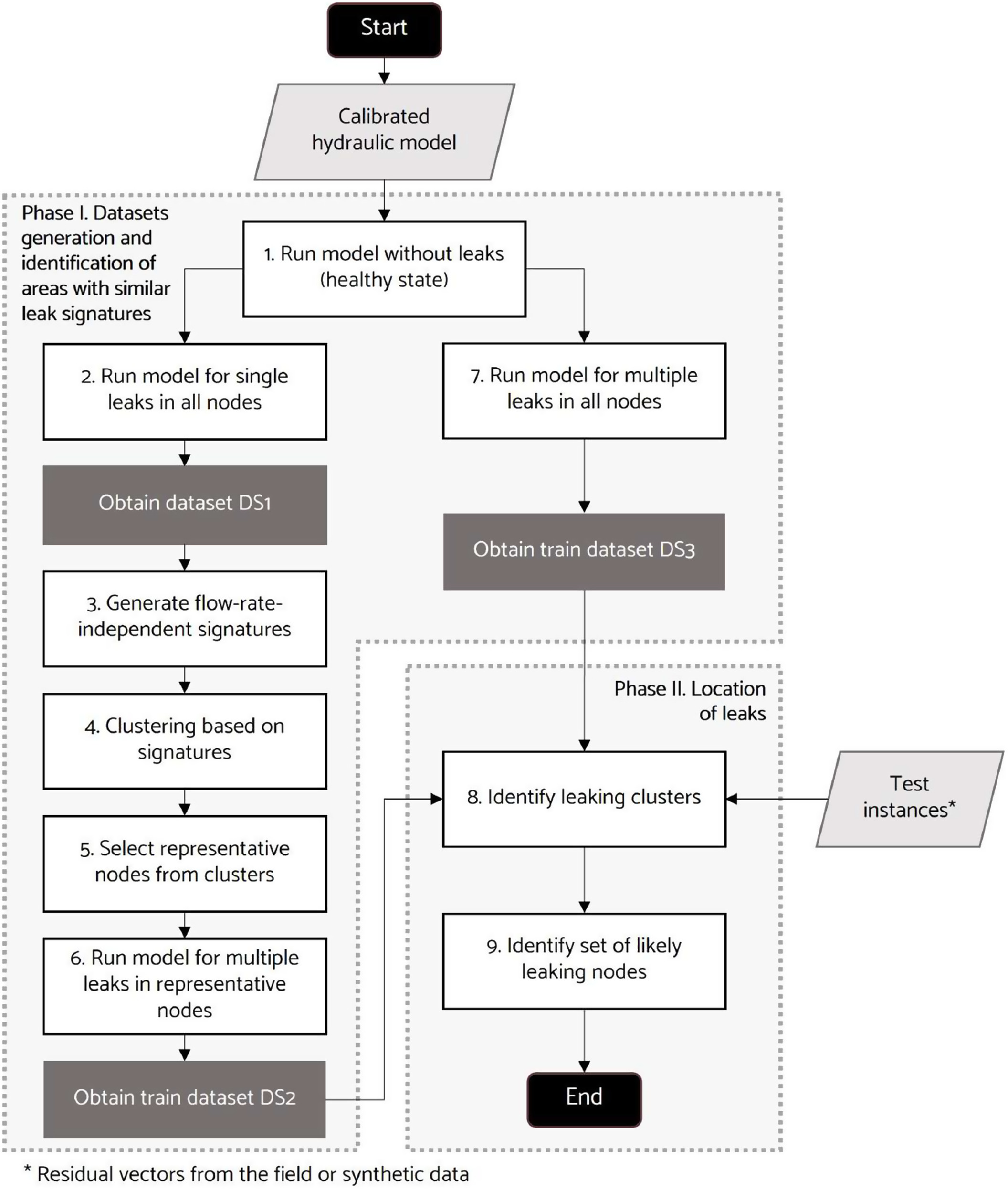
The proposed methodology consists of two phases, namely (1) data set generation and clustering, and (2) location of multiple leaks. The input for Phase 1 is a calibrated hydraulic model, and the input for Phase 2 is a list of values related to pressure data coming from sensors in the field, namely a test residual vector. The objective of the first phase is to generate three data sets to be used as inputs for Phase 2, whose final objective is to identify where the leaks are occurring. Fig. 1 shows, for both phases, the required inputs in the light gray data boxes, the generated train data in dark gray, and the steps to be performed in the open boxes.
We formulated leak location as a classification problem. Unlike single leaks, conceived as a multiclass problem, the allocation of more than one leak is a multiclass multilabel problem; hence, an instance receives more than one label representing the probable locations of the multiple leaks. The training data are represented by residual vectors constructed from various leak magnitudes and locations for all time steps. The classes of the training instances are the IDs of the leaking nodes. When a new instance (a residual vector obtained from field pressure measurements or from synthetic data) is presented to the trained classifier, it is categorized based on its similarity to the training instances, resulting in the identification of the most likely leaking nodes.
Phase 1: Data Set Generation and Identification of Areas with Similar Leak Signatures
This phase consists of seven steps (Fig. 1). Starting from the calibrated hydraulic model, the first step is to simulate the network condition with no leaks, namely, the healthy state. The pressure values obtained at the sensor nodes for all time steps are the baseline to calculate the pressure residuals for all leak scenarios. Twenty-four hourly time steps are considered to capture the pressure sensitivity throughout the day and reduce the number of false negatives.
The second step is to run the model while simulating individual leaks in each node as additional demands within a predetermined range of values. For this matter, a pressure-driven approach (PDA) is employed. Then, the pressure residuals for all sensor nodes are calculated by comparing the resultant pressure values in the leak scenario with those obtained for the healthy state, yielding the residual vectors for each modeled leak. A matrix () with representing the sensor nodes, corresponding to the number of simulated leaks, and corresponding to 24 hourly calculation time steps is produced. In this way, the first train data set (DS1) is obtained.
In the third step, the residual vectors are aggregated to obtain leak-flow-rate-independent signatures, used in the fourth step to create clusters. This aggregation is made considering that the residual vectors are inadequate for clustering, as they vary according to the leaks’ location and magnitude. By trimming down one of these dimensions, the leak flow rate, each leak location is given a distinctive vector (called a leak signature in the remaining text), which, unlike the residual vectors, is dimensionless and independent of the leak magnitude. Three strategies for aggregation are explored using DS1: one based on the leak flow rate [Eq. (2)], one based on the sum of the pressure residuals within the vector [Eq. (3)], and one based on the residual vector’s range [Eq. (4)]where = position within the vector; = aggregated result for each position ; = leak flow rate; and = each one of the pressure residuals. The criterion to assess the quality of the data aggregation is the variability of the results for different leak flow rates in a single leak location. The smaller the standard deviation for all positions in the residual vector, the more homogeneous the results; thus, the resulting signature represents better a given leak location.
(2)
(3)
(4)
Eq. (5) is used to assess the three signature aggregation strategieswhere AS = aggregation score; = number of nodes in the model; = number of sensor nodes; = number of simulated leaks; and = leak signature values. Because low scores indicate more homogeneous data and high aggregation scores indicate a significant divergence from the mean, the approach with the lowest AS among the signatures will be selected.
(5)
The obtained values for each residual vector are to be averaged to establish the leak location signature, . This way, the sample space is reduced from (number of leaking nodes) times (number of modeled leaks) residual vectors to signatures for clustering.
Step 4 is about generating the clusters based on the preceding signatures. Two clustering algorithms, -means (KM) and agglomerative hierarchical clustering (AH), are utilized, incorporating data preprocessing to capture the hydraulic response of the network. First, the undetectable nodes, those whose leaks do not impact any sensor nodes across all time steps, are separated because their signatures, which are made entirely of zeros, cannot be related to those from other nodes.
Next, the correlation matrix for the remaining nodes is calculated using the Pearson correlation coefficient (PCC). Nodes with low correlations below a threshold (0.95 in the case study) are excluded, requiring special attention from the water utility if a burst is detected. Afterward, the clustering algorithms are applied to the remaining nodes. AH is performed using PCC, Euclidian distance (ED), and cosine distance (CD). Leak location performs better when the nodes within a cluster are more similar to one another. To evaluate this similarity, the average signature for each cluster (relative to its centroid) is computed using Eq. (6)where = cluster; = value of the signature component in the position ; and = number of nodes in the referred cluster. Then, the correlation between each signature and the average signature of the correspondent cluster is calculated. The minimum value of all correlation coefficients is the clustering score (CS), as shown in Eq. (7), which is used to compare results between metrics. Finally, the metric with the highest CS is selected to run the AH algorithm and determine the optimal number of clusters ()
(6)
(7)
In Step 5, the node whose signature correlates better to the average of the signatures in its cluster is selected as representative for each group of nodes. In Step 6, multiple leaks are simulated in the representative nodes. To model two simultaneous leaks, one of them, called the base leak, remains placed in a certain node, and a second leak, called the dynamic leak, is simulated in the remaining nodes one at a time. Eventually, these leaks will converge at the same location, resulting in a single leak; this gives the model the chance of locating either single or multiple leaks. The residual vectors are built by comparing the pressure at the sensor nodes before and after the leaks. A matrix of columns and r rows is built, where is the number of sensor nodes and is the number of residual vectors. The result of this process is the train data set DS2. Step 7 is analogous to Step 2, although multiple leaks are simulated in all the model nodes, resulting in the third train data set (DS3). In this case we have simulated two simultaneous leaks.
Phase 2: Location of Multiple Leaks
This phase consists of two steps, identified as Steps 8 and 9 in Fig. 1. The detailed algorithm for these steps is presented in Fig. 2. In Step 8, the identification of the clusters containing the leaks occurs. To this end, the test residual vectors are computed at each time step by contrasting the pressure values at the sensor nodes in the leak scenario with those in the healthy state. All vectors concerning the undetectable nodes are excluded from the test set for two reasons. First, it is useless to search for a leak in the water network that is ostensibly nonexistent, and second, they increase the number of false negatives. Each test vector is compared with the individual vectors contained in DS2, and a similarity index is obtained using Eq. (8) (Corzo et al., unpublished data, 2022)where = similarity index concerning vectors and ; and = distance between them, which can be estimated using either the ED or CD. This procedure is completed for all time steps; then, the average similarity index is calculated for each residual vector in DS2. Only the maximum value remains for each representative node, and the clusters whose nodes obtain the highest values of are recognized as the areas containing the leaks.
(8)

The final step of the method is Step 9, to estimate where the leaking nodes are located. This process starts by filtering from DS3 the vectors produced by leaks in the previously selected clusters. Next, the test residual vectors are compared with the filtered training vectors for each time step, and the similarity indexes are calculated for all instances. Finally, the similarity values are averaged throughout all time steps, and the most likely leaking nodes are identified. Two criteria are used to this end. First, a fixed number of nodes: the nodes with the highest values are selected. Values of equal to three and five were previously used (Corzo et al., unpublished data, 2022) to evaluate the impact on the location accuracy while controlling the size of the set of leaking nodes. Second, a threshold for the similarity index is used: all nodes whose maximum similarity surpasses the defined threshold will be nominated. For this matter, the 95th percentile has been selected. When a threshold is considered, the number of identified nodes is variable. An advantage of using a threshold over a fixed number of nodes is that all nodes under identical maximum similarity conditions are considered.
Performance Assessment
Two metrics are used to assess the performance of the methodology. The first will assess leaking cluster identification. Because two exact values are expected, a helpful response should maintain the number of false positives low and the number of true positives high. For this reason, precision will be computed as the ratio between the number of true positives and the sum of true and false positives. The second metric uses accuracy () to assess the identification of the leaking nodes. This way, or a leak occurring in nodes and with flow rates and , respectively, can take the following values: if none of the actual leaking nodes is identified; if only one is pointed out, and if both nodes are identified.
Tools
Python Libraries
Several Python libraries have been involved in this research. Pandas (McKinney 2010) served to manage massive one-dimensional and multidimensional data sets. Scikit-learn (Pedregosa et al. 2011) was used to calculate the distance between residual vectors, and SciPy (Virtanen et al. 2020) and Yellowbrick (Bengfort and Bilbro 2019) were mostly employed for clustering. Furthermore, the Water Network Tool for Resilience (WNTR) (Klise et al. 2017) was used to perform all simulations and gather data from the hydraulic model. WNTR is built on EPANET and is compatible with its version 2.2 (Rossman et al. 2020), allowing the user to select a demand-driven approach (DDA) or a pressure-driven approach (PDA). All simulations in this paper used the latter.
High-Performance Computing
The computational demand increases when a second leak is introduced. Eq. (9) is used to estimate the number of simulations and the corresponding number of residual vectors () that result from simulating double leakswhere = number of nodes where the leaks are placed; = number of base leaks; and = number of dynamic leaks to be simulated. Due to the increase in the search space, the Dutch National supercomputer Snellius, hosted by SURF (2022)—a cooperative association of Dutch educational and research institutions, was utilized in various stages of this study. Snellius is the most powerful high-performance computing system in the Netherlands, offering powerful processing capabilities through parallel jobs, multiple cores, ample memory, and extensive storage space. It employs Simple Linux Utility for Resource Management (SLURM), a cluster management and job scheduling system (Jette et al. 2002).
(9)
SLURM is a centralized controller disk and execution monitor (daemon) that receives user commands and tasks, monitors resources, and distributes tasks to computing nodes. These nodes represent computers with multiple processors and cores, grouped into partitions based on hardware specifications. There are six partitions, each with a specific number of cores, memory, and maximum wall time, enabling the selection of the most suitable partition for job requirements.
Case Study and Experimental Setup
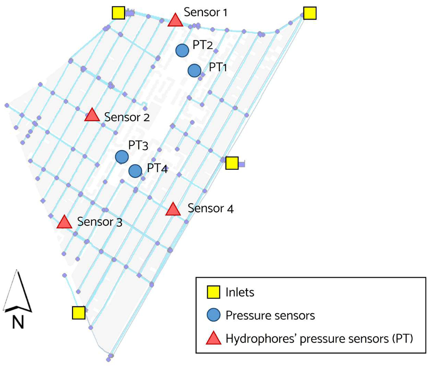
The proposed methodology has been applied in a DMA of a European town (López and Alfonso 2022). A DMA is used as a unit of analysis because of their advantages in terms of controlled boundary conditions for leak management. The hydraulic model of the DMA was initially simplified and subsequently calibrated. The simplification process involved the removal of unnecessary nodes from the network model. These nodes were identified as those without associated demand, those that did not represent changes in pipe characteristics, and those that did not contribute to the hydraulic performance of the network. The objective of this simplification was to reduce the sample space, resulting in a model comprising 144 nodes and 172 pipes. The total length of the pipes remained unchanged at 24.3 km. Asbestos cement is the predominant material, followed by high-density polyethylene (HDPE) and steel.
This district is fed by pumping stations located beyond the four entrances; thus, the intermediate distribution makes the head boundary conditions at the inlet nodes highly variable. Two inlets are mostly operational, whereas the others are turned on and off periodically. The district is fully instrumented; flow and pressure sensors have been located at the inlets, and eight pressure sensors are installed throughout the network; they are represented by nodes named Sensor1 to Sensor4 and PT1 to PT4. The nodes referred to as PT represent large consumers, namely, residential blocks fed by hydrophores. Fig. 3 shows the location of the current instrumentation in the DMA.
The proposed experiment aims to assess the methodology’s ability to accurately locate multiple leaks across a wide range of magnitudes, starting from two simultaneous instances. A hydraulic model was used to simulate single and double leaks, and the resulting pressure values were compared with those of a no-leak scenario. The resulting residual vectors were the testing instances that entered the classification model as inputs to identify the position of the leaks.
In order to generate the test data set, two nodes were randomly chosen from each cluster to form the test space and represent leaks. All possible combinations among these nodes using individual leaks ranging from 0.1 to were used in a manner that ensured the sum of the leaks remained within the range of the training data set. This process prevented any duplication of instances in the training data set. For detailed analysis, 15 leak intervals were determined based on the sum of individual magnitudes: (0.2–0.5), , nine intervals between 1.0 and with a range of , and four intervals between 10.0 and with a range of . The resulting test data set contains 40,170 instances, 2,678 for each interval.
Results
The results of the methodology applied in the case study are presented and discussed in the following subsections, with a focus on clustering (Phase 1, Steps 3–5) and multiple leak location (Phase 2, Steps 8–9).
Phase 1: Data Set Generation and Identification of Areas with Similar Leak Signatures
Following the methodology presented in Fig. 1, the calibrated model was run for the network’s current state (Step 1) and for the single leaks scenarios (Step 2), producing DS1 whose vectors are dependent on leak flow rates. However, because the leak magnitude is unknown, it is convenient to make the signatures independent from the flow rate by aggregating them (Step 3), so that it is possible to locate a leak regardless its leak magnitude. Three strategies to make this aggregation were assessed, namely by leak flow rate [Eq. (2)], by summing up pressure residuals within the vector [Eq. (3)], and by considering residual vector’s range [Eq. (4)]. Their application to DS1 yielded time-averaged aggregation scores AS [Eq. (5)] of 2.71, 29.87, and 88.96, respectively. For this reason, the aggregation by leak flow rate was adopted to generate the clusters.
The clustering methods were initially performed on the whole DS1. KM and agglomerative hierarchical clustering (AH) algorithms were evaluated using the silhouette coefficient and the elbow method measuring distortion. For KM, the elbow test pointed to seven clusters as the optimal value, and the maximum silhouette score corresponded to 11 clusters. For AH using CD, the optimal number of clusters was 4 and 11 for each method, respectively; however, the silhouette coefficients reached negative values. Scores below zero imply that some nodes might have been incorrectly assigned to a cluster.
Because low silhouette scores were expected given the multidimensionality of the data (Muller and Guido 2016), the resulting clusters were graphed in the DMA’s map to analyze the results in light of the network’s connectivity. Fig. 4 lists the findings for 7 and 11 clusters built by KM, AH using ED, and AH using CD. Even though the results were better for a higher number of clusters, the performance was inferior to expected. For instance, the algorithms failed to isolate the undetectable nodes. CD revealed better results than ED for all cases because the latter resulted in clusters occupying two separate areas, which is a nonadvisable situation.
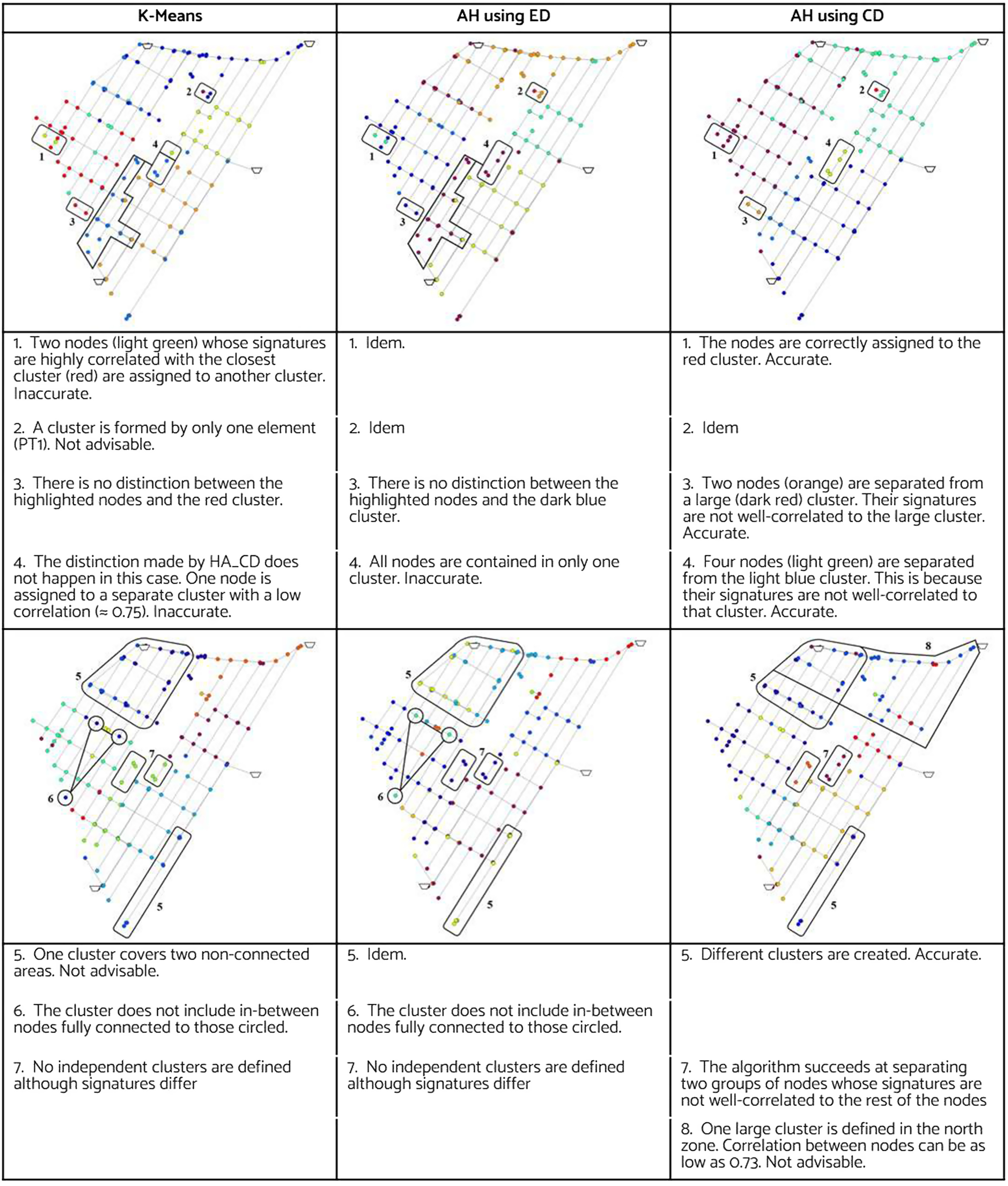
To execute the proposed improved clustering process, the five undetectable nodes (located in proximity to inlets and at dead-ends) were set apart together with six elements whose correlation coefficients for all nodes in DS1 were below 0.95. Because AH can employ PCC, ED, and CD, the results with the three metrics are compared through Eq. (7); PCC obtained the best results and was adopted to run AH.
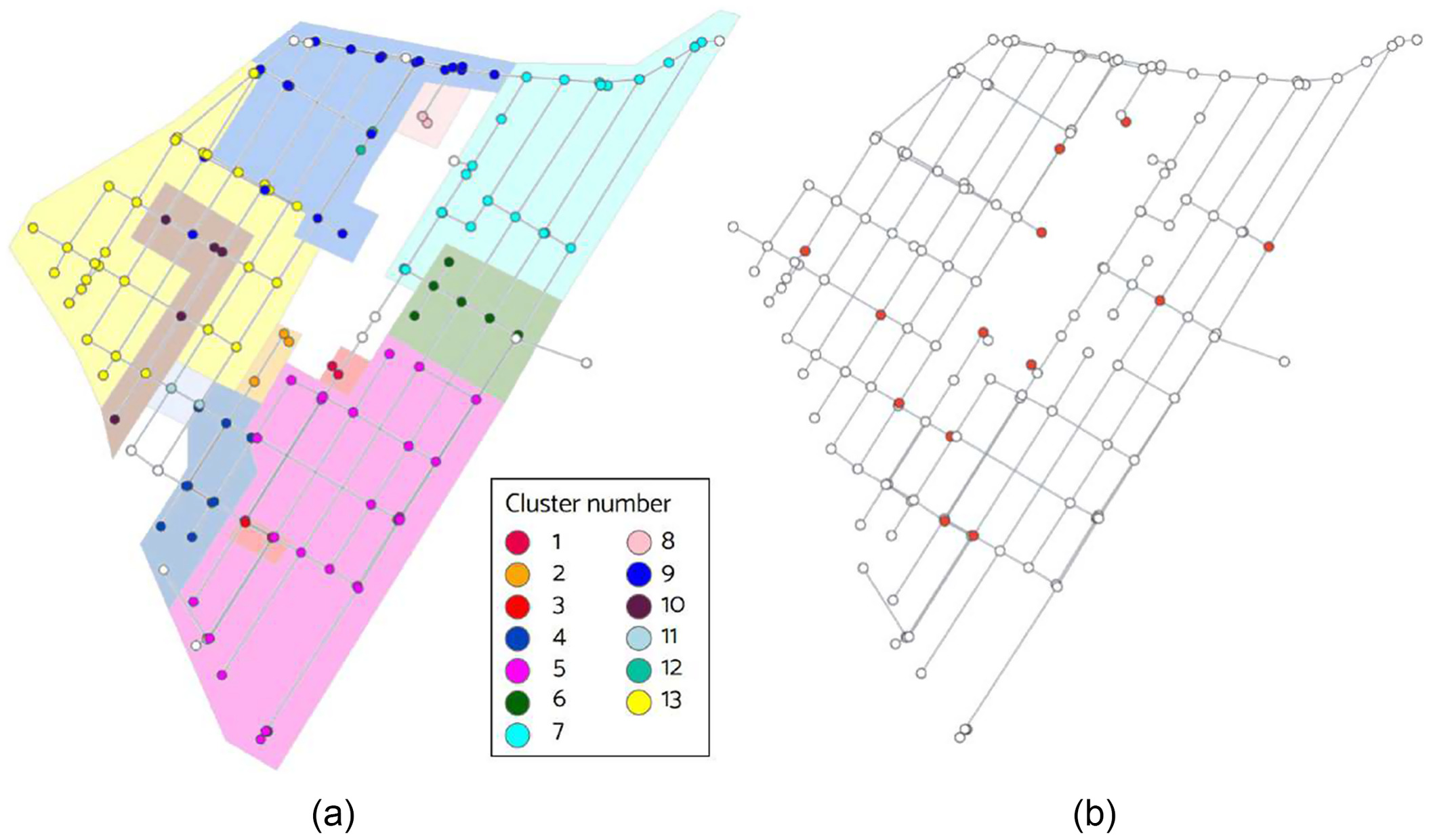
The clustering score was calculated for between 2 and 20. From two to six clusters there was a clear improvement in the score; above that value of , CS grew asymptotically to 1.0. The selected value of was 13 as it reached . The need to maintain small clusters for the case study was supported by the finding of significant variations between the signatures, despite the initial belief that clusters with two or three nodes should be avoided because they may decrease the effectiveness of the search.
Fig. 5(a) depicts the resulting clusters created by the proposed methodology using PCC as a metric for AH and K equal to 13. The polygons differentiate the clusters, and the open nodes represent undetectable nodes or those with a low correlation with the rest of the nodes. Once the clusters were determined, a representative node from each was selected (Step 5). The node with the strongest correlation to the cluster’s average signature was chosen as the cluster’s representative. Fig. 5(b) displays the cluster’s representative nodes. Multiple leaks were simulated in the representative nodes of each cluster (Step 6), resulting in DS2. A similar process was followed, although this time considering all noes in the model (Step 7), resulting in DS3.
Phase 2: Location of Multiple Leaks
At this point, all data required to locate the leaks are available. The 95th percentile criterion for node selection was introduced in the single-leak experiments previously presented by Corzo et al. (unpublished data, 2022) to compare the accuracy of the location of the leak with that obtained when a fixed number of nodes is used. In all cases, higher accuracy values were obtained using this threshold; consequently, this criterion was selected to be implemented in the multiple leaks’ experiment.
Fig. 6(a) presents the results of applying Steps 8 and 9. It shows how accurately the leaking areas and nodes were located for each leak flow rate interval using ED and CD. Two aspects are to be remarked upon regarding these results. First, there is a direct relationship between the leak magnitude and the location accuracy. For the case study, the accuracy in identifying the leaking areas that respond to the previously formed clusters soared from 0.2 to . It then continued growing at a lower rate, maintaining values over 80%. Accordingly, for this specific case, there was a clear threshold around , which that makes the difference for the water operator when identifying the leaking areas once a leak has been detected.
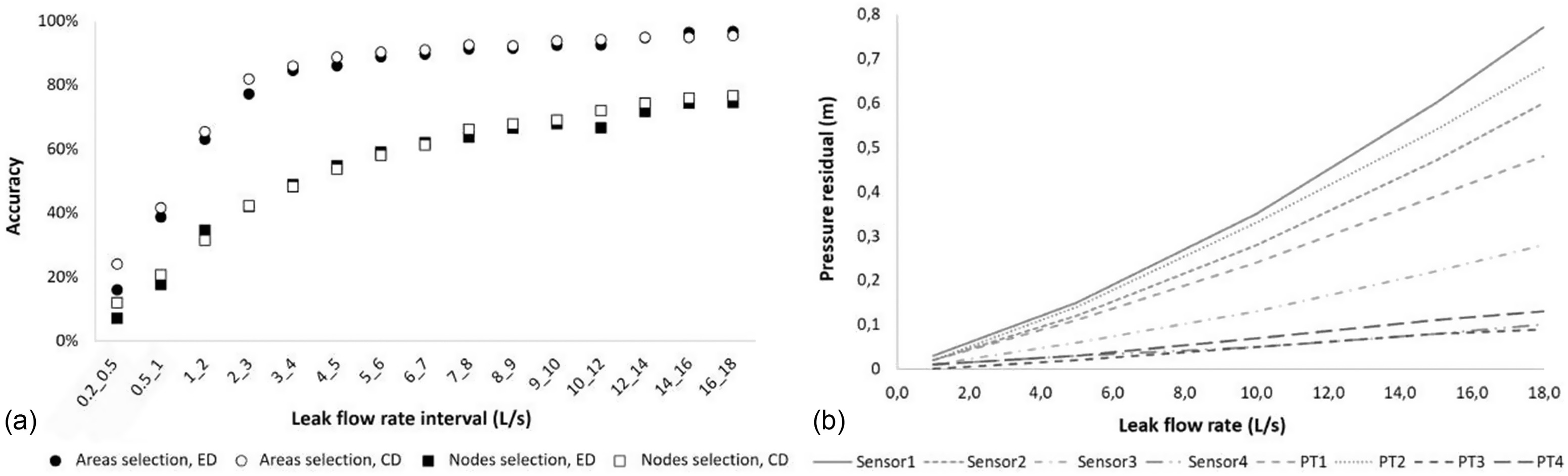
Oppositely, for the case study, there was no clear threshold regarding the location of the leaking nodes. Without such a stark divergence at the lower leak magnitudes, the accuracy of locating the nodes has a logarithmic trend. Accuracy values over 50% were obtained only when the sum of the individual leaks reached . Despite this, identifying the leaking area is still a valid step for the water operator to efficiently plan and execute the field pinpointing activities.
The second aspect refers to the differences in the results when different similarity metrics are used. In most cases using CD derives in better location accuracy values compared with ED, especially when low magnitude leaks are located. This is a crucial aspect to consider because leak location is more strongly needed for low flows, which are less likely to become visible.
Fig. 6(b) shows the change of the pressure residuals with the leak flow rate for a given leak location. Each leak or combination of leaks produces a specific set of curves. They are closer to each other for low leak flow rates, and they spread out as the leak magnitude increases. In consequence, the closeness of the curves at low flows makes it challenging to differentiate one set of curves from another, resulting in a higher number of nodes being selected and negatively impacting the accuracy. Oppositely, the more widespread the curves are, the better the distinguishability of the set of curves. It explains why higher leak magnitudes are related to better location accuracy values.
Nearly 70% of the leaking areas distinguished by the clusters (9 out of 13) were properly detected over 90% of the time for leaks above . Two more leaking areas crossed that line when the leaks’ combined magnitudes were roughly . The inflexion point noted in Fig. 6(a) was maintained in all cases because the location accuracy variation for combined leaks over was mostly stable. Nevertheless, the two remaining leaking areas did not reach 90% location accuracy even when large leaks were simulated. This poor response is directly related to their closeness to an inlet; any leak that develops in the inlet’s vicinity is immediately balanced and is not always detected by the pressure sensors.
Discussion
Factors Influencing Leak Location Accuracy
Three factors influencing the location accuracy were observed. First is the leak flow rate, where the larger the leak magnitude, the better the results. On the one hand, low leak magnitudes may produce pressure drops smaller than the sensors’ sensitivity. On the other hand, the closeness of the residual curves at low flows challenges the differentiation of one set of curves from another, resulting in a higher number of nodes being selected and affecting the accuracy. Second is the spatial location of the leak; in our case, the number of undetectable nodes decreases from 26 (18% of the DMA) for leaks below to five when leaks above were considered, showing that even for large leaks, some locations do not respond to pressure sensitivity.
The third,factor is the simulation period selected for the analysis. The more time steps that considered, the lower the number of false negatives obtained. Including multiple time steps is crucial for accurate leak detection because methods relying on a single time step may produce false negatives with zero-filled residual vectors, which are common to small leaks that, in low-flow scenarios, may not be able to produce enough friction losses to cause a detectable pressure drop. Therefore, a longer simulation period improves pressure sensitivity, enhancing the accuracy of leak detection.
Impact of the Similarity Criteria Used in the Methodology
Assuming that the pressure residuals vary linearly with leak flow rate, the proportions between the components of a residual vector tended to be constant for different leak magnitudes. It means that two residual vectors caused by two different leaks in a certain node will have different magnitudes but the same direction. The fact that ED considers the proximity of two multidimensional points whereas CD computes the angle between them explains why CD obtained better location accuracy in all experiments than ED, despite being more computationally demanding.
High-Performance Computing
The size and number of computations implied in the experiments required high-performance computing to allow for executing multiple parallel jobs. The initial action in this matter is to recognize what tasks can be parallelized and what computational resources are required to execute the processes and gain efficiency. In this paper, HPC was used for two main reasons. First, the size of the training and test data sets for multiple leaks involved large computational time. Rough estimations projected that the total computation time without parallelization would be above 110 days for Experiment B when cosine distance was used. Each parallel task was performed in about 24 h contemplating the whole test data set, on average. Second, even if time would not have been a limitation, loading and managing the training data for double leaks required higher RAM than available with other hardware resources. Whereas only 142 MB of RAM were required for this purpose when simulating single leaks, 47 GB were needed for double leaks. This may be a reason why comprehensive experiments were not attempted in previous studies.
Conclusions
This article presented a model-based data-driven approach to locate multiple leaks in water distribution networks using pressure residuals. It involved two phases, one to produce data sets to train the classification model and perform clustering, and the other to estimate the location of the leaks. Both phases form a methodology for detecting multiple simultaneous leaks considering previously overlooked variables such as the leak flow magnitudes and the simulation period considered in the analysis. The hydraulic model was used to generate data sets and adapt the data-driven model’s algorithms to the physics of the system, forming a hybrid model, which can be seen as the physics-aware data-driven model. This is a first step toward multiple leaks’ locations, which initiates with locating double leaks. This step is important because it considers the more realistic issue of multiple leaks occurring, instead of single leaks like any of the existing approaches.
We concluded that the accuracy of the leak location estimation is influenced by three main factors: (1) the magnitude of the leak, being directly related to the accuracy of the location estimation, (2) the spatial location of the leak, because it can be seen how some nodes remained undetectable even when large leaks, close to half the average demand of the DMA, were modeled, and (3) the length of the simulation period considered in the analysis, where the larger it is, the better results will be, because fewer false negatives are expected.
For the case study, we discovered a threshold for the sum of individual leaks of around , above which the accuracy of the leaking area location was greater than 80%, which is a good indicator for canalizing resources in the field. The specific conditions of a water distribution network may have an impact on the mentioned threshold.
Parallelization and HPC reduced computational time by 99%. Considering the length of the test set, instead of taking 110 days on a conventional computer, each partition only required an average of 24 h on HPC. This means that locating a leak in a network with similar conditions to the case study can be done within about half a minute for a single test instance. These results highlight the significant advantages of using HPC for analyzing multiple leaks.
Future research is advised on several fronts. First, further research is required in placing more simultaneous leaks, and comparing results with recent attempts involving deep learning methods. For this, HPC is crucial. Second, the accuracy of the location of the leaks may be influenced by the placement of sensors. It is important to evaluate to what extent they affect the estimations and confirm that undetected areas may arise from inconvenient sensor placement. Third, two other aspects are important to explore, namely, the duration and timing of the leak, and the addition of noise to demand or pressure sensor readings to reflect a more realistic situation.
Finally, the proposed approach proved to be applicable to the present case study, a WDN fed by multiple inlets. This is remarkable because the system is redundant, implying that pressure drops can be smaller than for single-sourced networks. This means that our methodology has the potential to have more accurate results for single-inlet systems. This is another avenue for future research.
Data Availability Statement
All data, models, or codes supporting the findings of this study are available from the corresponding author upon reasonable request.
Acknowledgments
This research is part of the NAIADES Project, which has received funding from the European Union’s Horizon 2020 research and innovation program under grant agreement No. 820985. This work was conducted on the Dutch national e-infrastructure with the support of SURF Cooperative. The Dutch Research Council (NWO) has funded its usage. Thanks are extended to Iulian Mocanu for providing the base hydraulic model and field data supporting the study case.
References
Ayadi, A., O. Ghorbel, M. BenSalah, and M. Abid. 2022. “A framework of monitoring water pipeline techniques based on sensors technologies.” J. King Saud Univ. Comput. Inf. Sci. 34 (2): 47–57. https://doi.org/10.1016/j.jksuci.2019.12.003.
Baader, J., P. Fallis, K. Hübschen, P. Klingel, A. Knobloch, C. Laures, E. Oertlé, R. Trujillo Alvarez, and D. Ziegler. 2011. Guidelines for water loss reduction–A focus on pressure management. Eschborn, Germany: Deutsche Gesellschaft für Internationale Zusammenarbeit.
Beal, C., and J. Flynn. 2014. The 2014 review of smart metering and intelligent water networks in Australia & New Zealand. Mount Gravatt, QLD, Australia: Griffith Univ.
Bengfort, B., and R. Bilbro. 2019. “Yellowbrick: Visualizing the scikit-learn model selection process.” J. Open Source Software 4 (35): 1075. https://doi.org/10.21105/joss.01075.
Candelieri, A., D. Conti, and F. Archetti. 2014a. “A graph based analysis of leak localization in urban water networks.” Procedia Eng. 70 (Jan): 228–237. https://doi.org/10.1016/j.proeng.2014.02.026.
Candelieri, A., D. Soldi, D. Conti, and F. Archetti. 2014b. “Analytical leakages localization in water distribution networks through spectral clustering and support vector machines. The icewater approach.” Procedia Eng. 89 (Jan): 1080–1088. https://doi.org/10.1016/j.proeng.2014.11.228.
Casillas, M. V., L. E. Garza-Castañón, and V. Puig. 2013. “Extended-horizon analysis of pressure sensitivities for leak detection in water distribution networks: Application to the Barcelona network.” In Vol. 8 of Proc., 8th IFAC Symp. on Fault Detection, Supervision and Safety of Technical Processes, 401–409. New York: IEEE. https://doi.org/10.23919/ecc.2013.6669568.
Chan, T. K., C. S. Chin, and X. Zhong. 2018. “Review of current technologies and proposed intelligent methodologies for water distributed network leakage detection.” IEEE Access 6 (Dec): 78846–78867. https://doi.org/10.1109/ACCESS.2018.2885444.
Erickson, J. J., C. D. Smith, A. Goodridge, and K. L. Nelson. 2017. “Water quality effects of intermittent water supply in Arraiján, Panama.” Water Res. 114 (May): 338–350. https://doi.org/10.1016/j.watres.2017.02.009.
Ferrandez-Gamot, L., P. Busson, J. Blesa, S. Tornil-Sin, V. Puig, E. Duviella, and A. Soldevila. 2015. “Leak localization in water distribution networks using pressure residuals and classifiers.” IFAC-PapersOnLine 48 (21): 220–225. https://doi.org/10.1016/j.ifacol.2015.09.531.
Jette, M. A., A. B. Yoo, and M. Grondona. 2002. “SLURM: Simple Linux utility for resource management.” In Proc., Job Scheduling Strategies for Parallel Processing (JSSPP) 2003, 44–60. Berlin: Springer.
Kapelan, Z., D. Savic, and G. Walters. 2003. “A hybrid inverse transient model for leakage detection and roughness calibration in pipe networks.” J. Hydraul. Res. 41 (5): 481–492. https://doi.org/10.1080/00221680309499993.
Klise, K., D. Hart, D. Moriarty, M. Bynum, R. Murray, J. Burkhardt, and T. Haxton. 2017. The water network tool for resilience (WNTR) user manual. Washington, DC: USEPA.
Li, R., H. Huang, K. Xin, and T. Tao. 2015. “A review of methods for burst/leakage detection and location in water distribution systems.” Water Sci. Technol. Water Supply 15 (3): 429. https://doi.org/10.2166/ws.2014.131.
López, E., and L. Alfonso. 2022. “Methodology to optimally place pressure sensors for leak detection in water distribution systems using value of information.” J. Water Resour. Plann. Manage. 148 (8): 04022043. https://doi.org/10.1061/(ASCE)WR.1943-5452.0001578.
McKinney, W. 2010. “Data structures for statistical computing in Python.” In Proc., 9th Python in Science Conf., edited by S. van der Walt and J. Millman, 56–61. Austin, TX: SciPy. https://doi.org/10.25080/Majora-92bf1922-00a.
Meseguer, J., J. M. Mirats-Tur, G. Cembrano, V. Puig, J. Quevedo, R. Pérez, G. Sanz, and D. Ibarra. 2014. “A decision support system for on-line leakage localization.” Environ. Modell. Software 60 (Oct): 331–345. https://doi.org/10.1016/j.envsoft.2014.06.025.
Muller, A., and S. Guido. 2016. Introduction to machine learning with Python: A guide for data scientists. Sebastopol, CA: O’Reilly Media.
OECD (Organisation for Economic Co-Operation and Development). 2016. “Water governance in cities.” Accessed June 26, 2022. https://www.oecd-ilibrary.org/content/publication/9789264251090-en.
Pedregosa, F., et al. 2011. “Scikit-learn: Machine learning in Python.” J. Mach. Learn. Res. 12 (Oct): 2825–2830.
Perez, R., et al. 2014. “Leak localization in water networks: A model-based methodology using pressure sensors applied to a real network in Barcelona.” IEEE Control Syst. 34 (4): 24–36. https://doi.org/10.1109/MCS.2014.2320336.
Perez, R., V. Puig, J. Pascual, J. Quevedo, E. Landeros, and A. Peralta. 2011. “Methodology for leakage isolation using pressure sensitivity analysis in water distribution networks.” Control Eng. Pract. 19 (10): 1157–1167. https://doi.org/10.1016/j.conengprac.2011.06.004.
Pudar, R. S., and J. A. Liggett. 1992. “Leaks in pipe networks.” J. Hydraul. Eng. 118 (7): 1031–1046. https://doi.org/10.1061/(ASCE)0733-9429(1992)118:7(1031).
Puust, R., Z. Kapelan, D. Savic, and T. Koppel. 2010. “A review of methods for leakage management in pipe networks.” Urban Water J. 7 (1): 25–45. https://doi.org/10.1080/15730621003610878.
Quevedo, J., M. Cugueró-Escofet, R. Pérez, F. Nejjari, V. Puig, and J. Mirats-Tur. 2011. Leakage location in water distribution networks based on correlation measurement of pressure sensors, 290–297. London: International Water Association.
Quiñones-Grueiro, M., M. Ares Milián, M. Sánchez Rivero, A. J. Silva Neto, and O. Llanes-Santiago. 2021. “Robust leak localization in water distribution networks using computational intelligence.” Neurocomputing 438 (May): 195–208. https://doi.org/10.1016/j.neucom.2020.04.159.
Quiñones-Grueiro, M., J. M. De Lázaro, C. Verde, A. Moreno, and O. Santiago. 2018. “Comparison of classifiers for leak location in water distribution networks.” IFAC-PapersOnLine 51 (24): 407–413. https://doi.org/10.1016/j.ifacol.2018.09.609.
Rossman, L., H. Woo, M. Tryby, F. Shang, R. Janke, and T. Haxton. 2020. EPANET 2.2 users manual. Washington, DC: USEPA.
Salguero, F. J., R. Cobacho, and M. Pardo. 2018. “Unreported leaks location using pressure and flow sensitivity in water distribution networks.” Water Supply 19 (1): 2018048. https://doi.org/10.2166/ws.2018.048.
Soldevila, A., J. Blesa, S. Tornil-Sin, E. Duviella, R. M. Fernandez-Canti, and V. Puig. 2016. “Leak localization in water distribution networks using a mixed model-based/data-driven approach.” Control Eng. Pract. 55 (Oct): 162–173. https://doi.org/10.1016/j.conengprac.2016.07.006.
SURF. 2022. “SURF is the collaborative organisation for IT in Dutch education and research.” Accessed July 12, 2022. http://www.surf.nl/en.
UN (United Nations). 2019. World population prospects 2019: Data booklet. ST/ESA/SER.A/424. New York: UN.
UN (United Nations). 2021. “The United Nations world water development report 2021.” United Nations, 2021 Edition. Accessed June 18, 2022. https://www.un-ilibrary.org/content/books/9789214030140.
Valizadeh, S., B. Moshiri, and K. Salahshoor. 2009. “Leak detection in transportation pipelines using feature extraction and KNN classification.” In Vol. 360 of Pipelines 2009: Infrastructure’s Hidden Assets, 580–589. Reston, VA: ASCE.
Van Der Walt, J., S. Heyns, and D. Wilke. 2019. “Pipe network leak detection: Comparison between statistical and machine learning techniques.” Urban Water J. 15 (10): 953–960. https://doi.org/10.1080/1573062X.2019.1597375.
Virtanen, P., et al. 2020. “SciPy 1.0: Fundamental algorithms for scientific computing in Python.” Nat. Methods 17 (3): 261–272. https://doi.org/10.1038/s41592-019-0686-2.
Wang, X., J. Li, S. Liu, X. Yu, and Z. Ma. 2022. “Multiple leakage detection and isolation in district metering areas using a multistage approach.” J. Water Resour. Plann. Manage. 148 (6): 04022021. https://doi.org/10.1061/(ASCE)WR.1943-5452.0001558.
Wu, Y., and S. Liu. 2017. “A review of data-driven approaches for burst detection in water distribution systems.” Urban Water J. 14 (9): 972–983. https://doi.org/10.1080/1573062X.2017.1279191.
Zhang, Q., Z. Wu, M. Zhao, J. Qi, Y. Huang, and H. Zhao. 2016. “Leakage zone identification in large-scale water distribution systems using multiclass support vector machines.” J. Water Resour. Plann. Manage. 142 (11): 04016042. https://doi.org/10.1061/(ASCE)WR.1943-5452.0000661.
Zhou, X., Z. Tang, W. Xu, F. Meng, X. Chu, K. Xin, and G. Fu. 2019. “Deep learning identifies accurate burst locations in water distribution networks.” Water Res. 166 (Dec): 115058. https://doi.org/10.1016/j.watres.2019.115058.
Information & Authors
Information
Published In

Journal of Water Resources Planning and Management
Volume 149 • Issue 12 • December 2023
Copyright
This work is made available under the terms of the Creative Commons Attribution 4.0 International license, https://creativecommons.org/licenses/by/4.0/.
History
Received: Oct 21, 2022
Accepted: Jun 30, 2023
Published online: Sep 19, 2023
Published in print: Dec 1, 2023
Discussion open until: Feb 19, 2024
ASCE Technical Topics:
- Algorithms
- Computer models
- Computer networks
- Computing in civil engineering
- Education
- Engineering fundamentals
- Infrastructure
- Lifeline systems
- Mathematics
- Models (by type)
- Pipeline systems
- Pipes
- Practice and Profession
- Pressure distribution
- Pressure pipes
- Training
- Utilities
- Water and water resources
- Water leakage and water loss
- Water management
- Water supply
- Water supply systems
Authors
Metrics & Citations
Metrics
Citations
Download citation
If you have the appropriate software installed, you can download article citation data to the citation manager of your choice. Simply select your manager software from the list below and click Download.