Abstract
The Colorado River’s two largest reservoirs are drawing down because releases exceed inflows and releases adapt to reservoir elevations instead of to elevation and inflow triggers. To help slow reservoir drawdown and sustain target elevations, we introduce a new rule that adapts basin depletions to available water. We simulated inflow-based operations and validated existing operations in a new open-source exploratory model for the Colorado River Basin. We developed the exploratory model to more easily adapt Upper and Lower Basin depletions to available water, reduce run time, and lower costs to use compared with the proprietary RiverWare Colorado River Simulation System (CRSS) model. We simulated adaptive and existing operations for (1) the 2000–2018 period, and (2) scenarios of steady Lees Ferry natural inflow each year of (bcm) [14–5 million acre-ft (maf)] per year. We found the following: (1) the existing rules drew down Lake Powell and Lake Mead to their critical storages of 7.4 bcm (6.0 maf) in less than 5 years when Lees Ferry natural flow was less than () (the 2000–2018 period average); and (2) the adaptive rule sustained both reservoirs above their critical levels for long periods by requiring Upper and Lower Basin users to conserve as much as 1.2 bcm (1.0 maf) per year more water than existing operations. The next steps should be testing the adaptive rule in CRSS and devising conservation programs that can adapt and scale to available water.
Introduction
The Colorado River supplies the two largest reservoirs in the country and flows through iconic landscapes such as the Grand Canyon and other National Park units. Management of the river is governed by a binational treaty, two interstate compacts, Supreme Court decisions, laws and administrative rules, and numerous interparty agreements collectively called the Law of the River. The Law of the River began to be codified in the 1920s, when the Colorado River Compact was negotiated (Hundley 1975; Kuhn and Fleck 2019), and the compact intends to provide certainty about the volume of water that basin states and users can divert. Today, two of the largest reservoirs are drawing down because consumptive uses has exceeded the decreasing basin runoff (Woodhouse et al. 2016; Udall and Overpeck 2017; Xiao et al. 2018; Hoerling et al. 2019; Milly and Dunne 2020), which has renewed concerns about how to allocate a diminishing and uncertain supply. Basin managers, stakeholders, and others need tools to help them manage the reservoir system in more adaptive, transparent, and sustainable ways in the face of hydrologic and other uncertainties.
Three major types of models currently are used for reservoir management: optimization, simulation-based optimization, and simulation and rule-based simulation. A reservoir optimization model searches for reservoir releases and reservoir elevations that maximize benefits (e.g., hydropower generation revenue) or minimize cost (e.g., water supply cost) given a set of constraints (e.g., water balance equations). These models can help identify optimal or near-optimal solutions, especially when system objectives are clear. Draper et al. (2003) developed the California Value Integrated Network (CALVIN) to help identify statewide reservoir storage, releases, and flows to minimize California’s water supply cost. In this model, inflow was assumed to be perfectly known, and the Hydrologic Engineering Center Prescriptive Reservoir Model (HEC-PRM) software, which solves linear programs with a network structure, was adopted to solve the model. Dogan et al. (2018) introduced the Python-based CALVIN model, which is coupled to multiple linear programming solvers. This open-source model provides more flexibility by investigating limited forecast optimization and comparing runtime benchmarks for different linear solvers.
In a simulation-based optimization model, operating policies are tested in a simulation model first and then adjusted by optimization techniques in each iteration to improve system productivity, increase efficiency, or reduce system cost. Knox et al. (2018) proposed a Python network simulation (Pynsim) framework for multiagent simulation of networked resource systems. This model enables users to connect to other models and incorporates an example coupling with multiobjective evolutionary algorithms to explore Pareto-optimal solutions among different objectives.
Rule-based simulation models simulate system performance with predefined operating policies. They allow users to define and test multiple different operating policies against many hydrologic and demand scenarios. The USACE Hydrologic Engineering Center developed HEC-ResSim to simulate reservoir operations for flood control, water supply, and other purposes (Klipsch and Evans 2006). RiverWare is another widely used proprietary rule-based simulation software in which a river basin’s network of dams and diversions are represented and edited using a graphical user interface (Zagona et al. 2001). In the Colorado River, the Bureau of Reclamation maintains the RiverWare Colorado River Simulation System (CRSS), which represents the water supply and river network with 12 reservoirs, 29 inflow nodes, 520 water user objects, and 145 primary rules (Wheeler et al. 2019). Stakeholders with substantial technical expertise and budget resources use CRSS to explore alternative long-range strategies to manage water supplies and demands. However, testing different alternative management policies with CRSS is challenging because many policies in CRSS are closely related and one must be careful to make the right changes to the policies. In addition, there are many water-user objects in CRSS, and one must assign correct demand shortages to each individual user.
Among many of those alternative management policies, adaptive reservoir management policies gain more and more attention as they adapt policies or decisions over time as conditions change and information improves (Haasnoot et al. 2013; Herman et al. 2020; Wang et al. 2020; Yang et al. 2021). Signposts usually represent undesirable system conditions or expiration dates, and often are used to determine when and under what conditions to adapt operations. In the Colorado River, the Lower Basin’s Drought Contingency Plan (DCP) has two adaptive features: (1) conservation targets increase as the Lake Mead elevation drops, and (2) to avoid further lake elevation drops, delivery of Intentional Created Surplus water is not permitted when the Lake Mead elevation is projected to fall below 312 m (1,025 ft). Similarly, the Upper Basin DCP pledges to protect Lake Powell’s elevation of 1,074 m (3,525 ft) to minimize the risk of hydropower generation failure. All these operations adapt releases to reservoir elevations, not inflow.
To help slow reservoir drawdown, we present an exploratory rule that adapts basin depletions to inflows. The rule triggers at a higher Lake Mead elevation, 323 m (1,060 ft), and dynamically sets system depletions equal to inflows. We validated the existing operations and simulated the new rule in an open-source exploratory model for the Colorado River Basin. We developed the model to more easily adapt Upper and Lower Basin depletions to available water, reduce run time, and lower costs to use compared with CRSS. We used the model to identify the inflow and demand conditions and operations for which the system is vulnerable. This paper contributes
•
an adaptive policy (ADP) that adapts basin depletion to streamflow;
•
an exploration of Colorado River system vulnerabilities under declining hydrologic conditions;
•
an evaluation of ADP and DCP for Lees Ferry natural flow scenarios that range from 17.3 to (bcm) [14–5 million acre-ft (maf)] per year; and
•
an open-source, exploratory Python model for the Colorado River system.
Section “Open-Source Exploratory Model Description” introduces the exploratory model. Section “Case Study: Colorado River Basin” presents the Colorado River case study, including the model structure, current operations, and rule that adapts to basin inflows. Section “Example Results” shares example results for model validation, sensitivity analysis, and reservoir simulations of adaptive policies across hydrologic scenarios. Section “Limitations and Future Works” presents limitations and future work. The final section summarizes our contributions to adapting depletions to inflow and slowing reservoir drawdown.
Open-Source Exploratory Model Description
Open-source exploratory models provide data, model, code, and directions for use in a public repository without promise of or budget for ongoing support. This contrasts with a paid, proprietary model such as RiverWare/CRSS, for which payment also grants the user access to technical support. The open-source exploratory model in this research uses object-oriented programming to classify different kinds of objects, such as reservoirs, users, and rivers. Python was selected as the programming language because (1) more and more water resource scientists are using Python (Knox et al. 2018; Smith et al. 2018; Díaz-González et al. 2021), (2) it enables object-oriented programming, (3) it supports a large number of data processing and plotting libraries, and (4) it is an open-source programming language. The exploratory model, developed based on Python, is available to download, and results from this research are reproducible (see the “Data Availability Statement” and “Reproducible Results” sections).
Basic Setup and Running a Simulation
The exploratory model is a generic simulation model. The object-oriented programming allows users to build a network in a structured way, the open-source feature provides users the ability to code unique features and model behaviors, and Python libraries provide tools for fast data processing. Building a customized model and running a simulation with the exploratory model mainly involves four steps.
1.
Develop a water resources system network by creating instances of reservoirs, users, and rivers classes. The exploratory model structures the system as a network, which consists of nodes and links. A node can represent a reservoir or a user. The Reservoir node class (defined in Reservoir.py) is the parent class for all reservoirs, and it includes basic properties such as elevation, storage, inflow, outflow, spill, and so forth. This class also provides some basic functions, such as converting from storage to elevation. The User class (defined in User.py) has a demand property to represent how much water is required in each time step. Failure to meet this demand is defined as water shortage. A link connects two different nodes. The River class (defined in River.py) links two nodes from upstream to downstream. More-specific reservoir, user, and river classes can be defined, and they will inherit properties from the three base classes.
2.
Specify input param and scenarios. Similar to many other rule-based simulation models, the exploratory model requires input of basic reservoir param, inflow scenarios for each reservoir, and demand scenarios for each water user, as well as system setting parameters such as planning horizon and start and end dates of simulation. Data input functions are defined in DataExchange.py and utilize Python’s Pandas library to import the data stored in the data folder.
3.
Develop operating rules to specify when and how much water to release from each reservoir. In the exploratory model, all operating rules are defined in ReleaseFunction.py, and their active states are controlled in the policyControl.py script. Users are allowed to develop their own operating rules by expanding the ReleaseFunction.py script. Because all reservoir simulation data and results are assigned and calculated within the network object, the operating rules can access the latest system information within the network to determine how much water users should conserve and how much water to release from reservoirs. This exploratory model is allowed to create traditional policies such as rule curves or release rules that are related only to reservoir elevations. It also is suitable for the adaptive policies that utilize the latest information and are based on both inflow information and reservoir conditions.
4.
Simulate scenarios and output results. Simulations start by running the start.py script in the simulation folder. The model then uses the defined rules to simulate the system from the beginning to the end of the planning horizon from upstream reservoirs to downstream reservoirs across specified hydrologic and demand scenarios. After simulation, the exploratory model exports reservoir inflows, elevations, storages, releases, user demands, and shortages to the results folder. Data output functions are defined in DataExchange.py and adopt Python’s xlwt library to export all those results. Users are allowed to change the default export setting and customize the results to export by adding more data output functions in DataExchange.py.
Sensitivity Analysis
Multidimensional uncertainty analysis can reveal the effects of multiple uncertain factors on the activity or system of interest. It was used by Brown et al. (2012) to help understand how decisions are sensitive to uncertain changing precipitation, temperature, and other factors. The exploratory model provides such a tool to help identify the combinations of future streamflow, user demands, and operating policies that push the system into vulnerable or undesirable states. The insights from sensitivity analysis can help guide when and how to adapt operating policies to avoid system failure. In the exploratory model, to initiate a multidimensional uncertainty analysis, first the inflow ranges and different demand levels are specified in SensitivityAnalysis.py, then user polices are defined in ReleaseFunction.py, and finally the policies are simulated under different combinations of inflows and demands in start.py. Results from this process can help identify (1) under what conditions and how long the system will fail, and (2) policies that reduce failures or more quickly recover the system.
Case Study: Colorado River Basin
The Colorado River Basin encompasses approximately 8% of the continental US, and provides water supply, irrigation water, and hydroelectricity to 40 million people in the US and Mexico. River management in the early and mid-20th century focused on water supply and hydroelectricity production, whereas modern management also considers ecosystem services provided by the river, native and endemic species that are endangered or threatened, and protection and enhancement of National Park System units. Many factors will affect the future management of the Colorado River, including increasing air temperature, decreasing watershed runoff, population growth, changing patterns of consumptive use, preferential filling of some reservoirs, changes in river ecosystems, changing societal values, evolving water allocation policies, and the location and extent of water conservation efforts. Many of these factors are difficult to predict, especially several decades into the future.
Reservoir Simulation Model (Structure and Data)
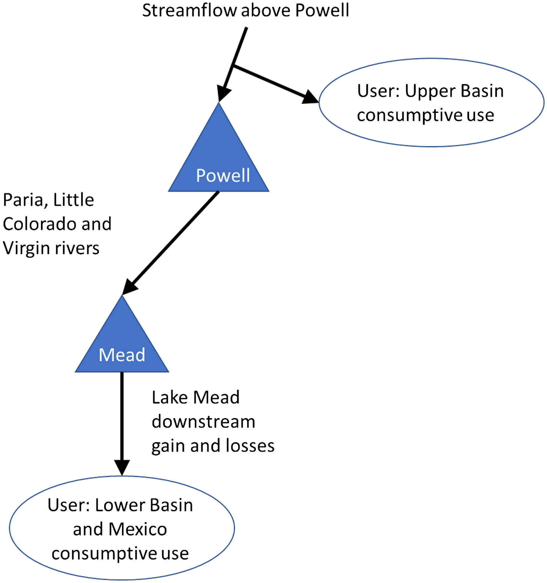
In the exploratory model for the Colorado River Basin, two reservoirs, Lake Powell and Lake Mead, account for approximately 83% of the entire basin storage volume. There are two aggregated users: the Upper Basin, and the Lower Basin and Mexico (Fig. 1). In this example, three upper basin tributaries (Upper Colorado River, Green River, and San Juan River) were aggregated into one tributary to Lake Powell, and three tributaries (Paria River, Little Colorado River, and Virgin River) were aggregated into one tributary to Lake Mead. Lake Mead downstream gains and losses include inflow below Lake Mead, changes to Lake Mohave and Lake Havasu storage, and evaporation losses. All individual Upper Basin users were combined into one Upper Basin user (UB), and all Lower Basin and Mexico users were combined into one Lower Basin user (LB and Mexico). We assumed that the combined Upper Basin user consumes water above Lake Powell, and that the combined Lower Basin user consumes water below Lake Mead and its downstream gain and losses.
The exploratory model simulates reservoirs from upstream to downstream. For each reservoir, the water balance equation—inflows minus releases minus evaporation equals change in storage—is applied to simulate the changes in reservoir storage based on different operating rules. In the exploratory model, all basic param for Lake Powell and Lake Mead were obtained from the August 2020 version of CRSS. In CRSS, evaporation for Lake Powell is calculated using a periodic net evaporation method, and Lake Mead evaporation is the product of reservoir surface area and evaporation rates. To be consistent with CRSS, we used the same method in the exploratory model.
The Direct Natural Flow scenario from 1906 to 2018, which had () mean natural flows at Lees Ferry, was incorporated into the exploratory model. This scenario includes the mid-20th century drought from 1953 to 1977, with () mean natural flows at Lees Ferry and the Millennium Drought from 2000 to 2018, with () mean natural flows at Lees Ferry. In the Direct Natural Flow scenario, the index sequential method (Kendall and Dracup 1991; Ouarda et al. 1997) is applied to generate 113 hydrologic traces. This scenario is provided by the US Bureau of Reclamation and is used in CRSS (August 2020 version). For sensitivity analysis, we used scenarios of Lees Ferry natural flow that ranged from 17.3 to () each year and were observed in the tree-ring reconstructed flow record from 1416 to 2015 (Salehabadi et al. 2020). This range captures long-term droughts such as the mid-20th century drought and the Millennium Drought, and it also captures short-duration droughts such as the extreme dry year 2002 [ ()] and the 2012–2013 drought sequence [ ()]. We assumed that average intervening inflow below Lake Powell was () (Wang and Schmidt 2020), which included tributaries within the Grand Canyon and streamflow from the Virgin River.
We used an increasing UB demand scenario projected by the Upper Colorado River Commission (UCRC 2007) that also is the default demand schedule in CRSS (August 2020 version). In addition to the LB and Mexico demand schedule, Lake Mead also needs to release water to meet LB gains and losses (including inflow below Lake Mead, changes to Lake Mohave and Lake Havasu storage, and evaporation losses). These data used in the exploratory model varied among different streamflow traces, and all were obtained from CRSS (August 2020 version). In sensitivity analysis, average UB demand was assumed to be 6.6 bcm (5.35 maf) per year (UCRC 2007, schedule B), and average LB and Mexico demand was assumed to be 11.8 bcm (9.6 maf) per year (Fleck 2020) (Table 1).
| Basin | State | Average annual consumptive uses and losses [ ()] |
|---|---|---|
| Upper Colorado River | Colorado | 3.59 (2.91) |
| Wyoming | 0.89 (0.71) | |
| New Mexico | 0.78 (0.63) | |
| Utah | 1.34 (1.08) | |
| Upper Basin total | 6.6 (5.35) | |
| Lower Colorado River and Mexico | Arizona | 3.45 (2.8) |
| California | 5.43 (4.4) | |
| Nevada | 0.37 (0.3) | |
| Lake Mead downstream regulation and gains and losses | 0.74 (0.6) | |
| Mexico | 1.85 (1.5) | |
| Lower Basin and Mexico total | 11.84 (9.6) |
Adaptive Policy and Drought Contingency Plans
In the current version of the exploratory model, we replicate seven important CRSS Lake Powell operating rules that equalize Lake Powell and Lake Mead storages under different elevation tiers defined in the 2007 Interim Guidelines (USBR 2007). In addition to these rules, the exploratory model also provides a compact version of the equalization rule that uses fewer parameters than the replicated rules. In this rule, Lake Powell releases are iterated to balance Lake Powell and Lake Mead. The 2007 Interim Guidelines, Drought Contingency Plan (USBR 2019), and International Boundary and Water Commission (2012, 2017) determine LB and Mexico contributions (or cutbacks) under different Lake Mead elevations; the lower the elevation, the larger is the cutback. In the exploratory model, a nested if-else statement is used to return increasing cutback values as Lake Mead elevation falls from 332 to 312 m (1,090 to 1,025 ft). A new rule returns cutbacks 1.5 bcm (1.2 maf) per year larger than the DCP for the same elevation tier. This rule goes further than a December 2021 pledge by the Lower Basin states to conserve an additional 0.6 bcm (0.5 maf) each year for 2 years (USBR et al. 2021).
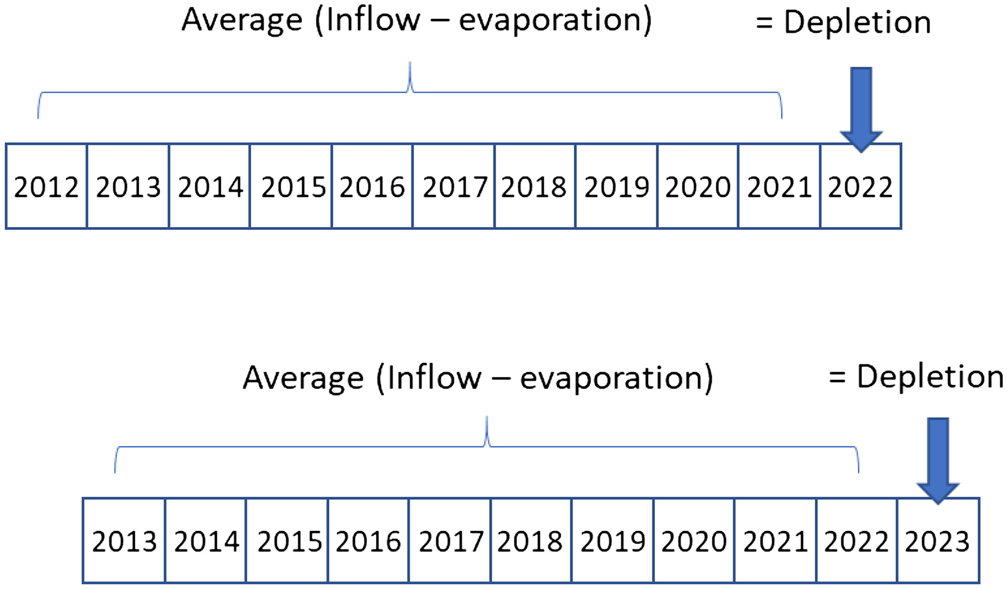
The adaptive policy in this research was defined as adapting depletion to the average past 10-years of system gain (Fig. 2). Gain is the difference between inflow and reservoir evaporation. The ADP uses the most recent hydrologic information every year to assist with the next year’s decision-making regarding depletions and reservoir storage. The benefits to using hydrologic information from several past years include the following: (1) it allows users to use only the available water coming into the system; (2) it dynamically balances basin depletion and water system gains; (3) it captures recent hydrologic changes; (4) it uses the most recent data; and (5) it prevents severe reservoir drawdown during one or more low inflow years. Water conserved in reservoirs still belongs to users, and can be used when severe drought occurs. Eq. (1) assumes that next-year depletion for the entire basin is equal to the average past gains to the systemwhere = total water depletion in year ; = inflow in past year ; = evaporation in past year ; = total years to look backward; and to = lookback period.
(1)
Water shortages in the coming year are calculated by subtracting the total system depletion determined using Eq. (1) from the original basin demand schedule. Many strategies exist to allocate entire basin shortages to UB or LB and Mexico. We tested different strategies ranging from the UB bearing all shortages to the UB bearing no shortages. In this research, we simulated the ADP strategy along with the equalization policy (to determine where to store water) across all historical streamflow records (1906–2018). The ADP strategy is assumed to start in January 2021 and will be triggered only when Lake Mead elevation is less than 323 m (1,060 ft) and the average system gain over the last 10 years is smaller than the next year’s demand schedule. Selecting 323 m (1,060 ft) creates a buffer before Lake Mead drops below 312 m (1,025 ft). When Lake Mead elevation is above 323 m (1,060 ft), LB and Mexico contributions are calculated by the DCP operation. The 323 m (1,060 ft) trigger is 10.7 m (35 ft) and 3 bcm (2.4 maf) higher than the 312 m (1,025 ft) trigger in the Lower Basin DCP. Managers can trigger the adaptive rule at higher or lower elevations. Triggering at a higher elevation will reduce depletions earlier and leave more water in the reservoir.
Example Results
Model Validation
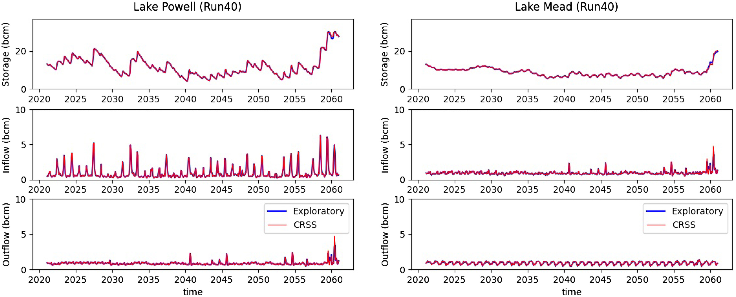
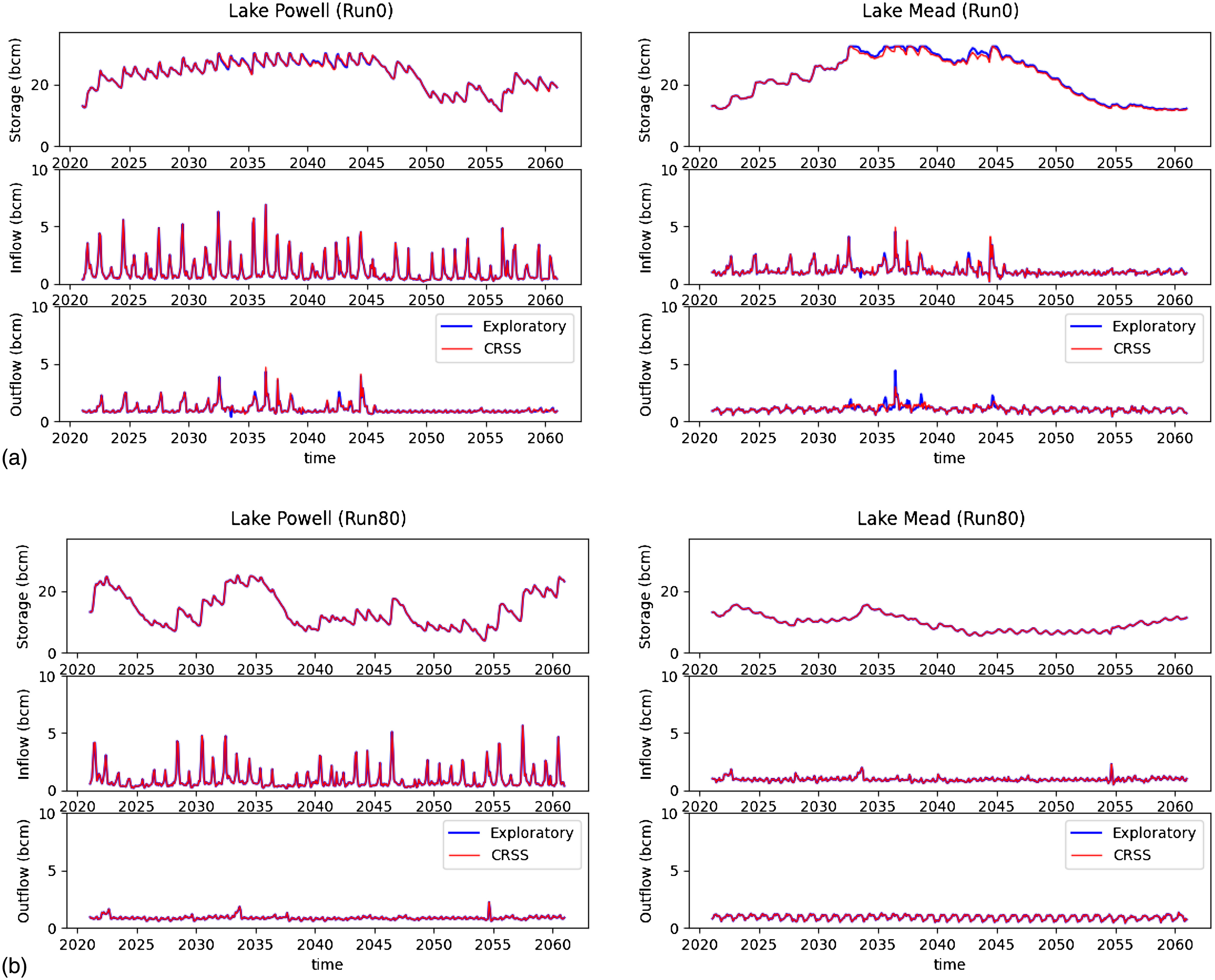
To validate the exploratory model, we set the values for Lake Powell inflow and intervening Lake Mead inflow, starting storage, maximum releases, demands, and operating rules in the exploratory model to be the same as the values in the August 2020 version of CRSS (Appendix). Results for one hydrologic trace that repeated a mid-20th century drought show that simulation results for Lake Powell and Lake Mead storage, inflow, and outflow from the exploratory model were very close to those of CRSS (Fig. 3). The average flow at Lees Ferry during this mid-20th century sustained drought (1953–1977) was (12.89 ), which was 87% of the long-term average from 1906 to 2018 (Salehabadi et al. 2020). Validation results for other hydrologic traces also were similar (Appendix). The computational time for each hydrologic trace in the exploratory model was about 0.35 s, which is 50 times faster than the CRSS single-trace run time of about 20 s in the same computational environment (single-core testing with Intel Core i7-9850H CPU at 2.60GHz). Minor differences between the exploratory model results and CRSS results were due to the exploratory model replicating many important policies in CRSS, but not all of them (Appendix). These validation results demonstrate the capability of the exploratory model to simulate correctly the two largest reservoirs in the Colorado River system.
Multidimensional Sensitivity Analysis
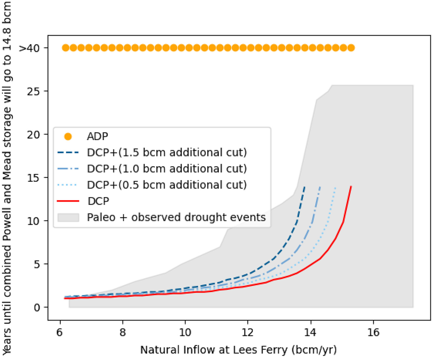
We used the sensitivity analysis tool introduced in the section “Sensitivity Analysis” to analyze system performance under different natural flows at Lees Ferry, user demands, and release policies. Under many scenarios in which Lees Ferry natural flow ranged from 6.2 to 15.3 bcm (5–12.4 maf) every year, the existing Lower Basin DCP operations drew down the combined storage of Lake Powell and Lake Mead to 14.8 bcm (12 maf) in less than 5 years (Fig. 4). We selected the combined 14.8 bcm (12 maf) storage threshold because it represented drawdown to 7.4 bcm (6 maf) of storage in each reservoir, which are the elevations to protect the minimum power pool for Lake Powell [1,074 m (3,525 ft)] and the lowest operation tier in the Drought Contingency Plan for Lake Mead [312 m (1,025 ft)]. With natural flow of 15.3 bcm (12.4 maf) at Lees Ferry every year, increasing the largest DCP cutback by 1.5 bcm (1.2 maf) per year over the existing cutback pushes the drawdown time to about 20 years. However, with natural flow of 12.3 bcm (10 maf) or lower at Lees Ferry every year, all versions of the DCP drew down combined reservoir storage to 14.8 bcm (12 maf) in about 3 years or less. The shaded section in Fig. 4 shows the numerous combinations of event duration and natural flow volume at Lees Ferry that occurred in the observed and paleo records (Salehabadi et al. 2020, Fig. 14). These numerous hydrologic scenarios are possible and quickly can draw down reservoir storage to critical levels. The solid and dashed lines in the shaded area indicate that DCP and DCP+ will not get the LB, Mexico, or UB through many hydrologic events from the observed and paleo records.
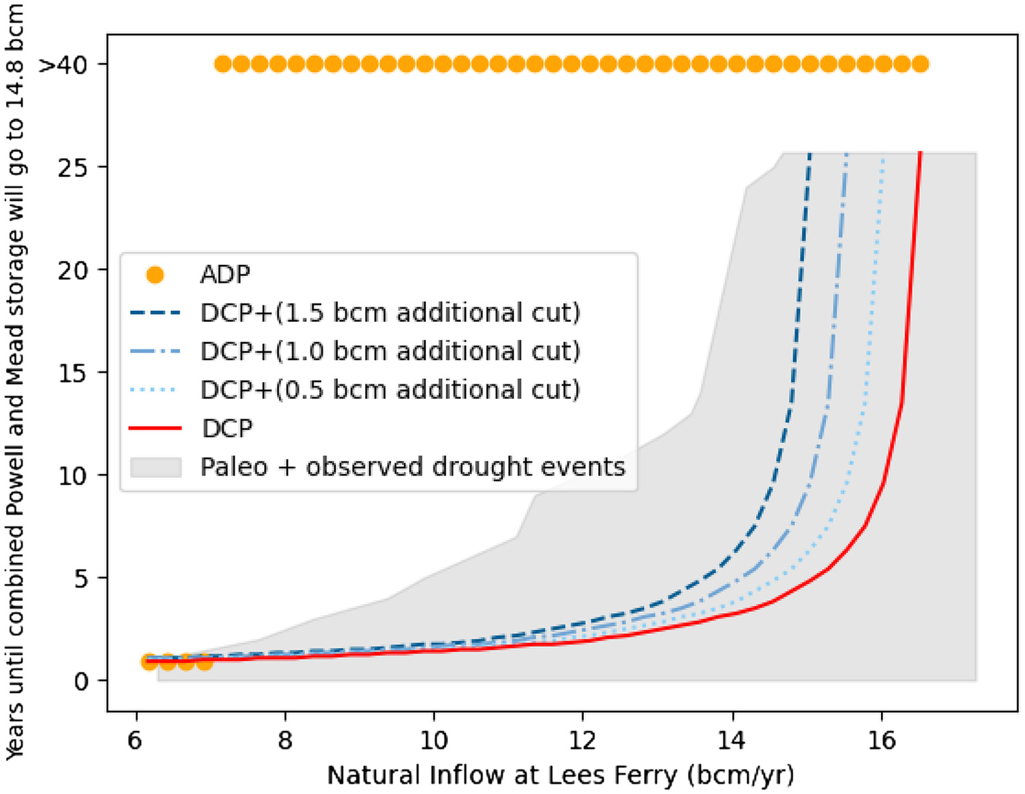
In contrast, the ADP keeps combined reservoir storage above 14.8 bcm (12 maf) for 40 years or longer for Lees Ferry natural flows above 6.2 bcm (5 maf) per year each year. For Lees Ferry natural flow of about 6.2 bcm (5 maf) per year each year, the ADP does not maintain combined storage above 14.8 bcm (12 maf) because the reservoir storage falls below 14.8 bcm (12 maf) before the ADP rule is triggered. The ADP rule sustains reservoir levels through much longer droughts than do the current DCP operations. The ADP rule sustains reservoir levels because the ADP rule adapts and cuts back depletions to the available gains to the system—the inflow minus evaporation. In contrast, the DCP operations and variants cut back depletions according to a lower fixed lake level schedule that does not consider annual reservoir inflow. In short, the ADP requires users to conserve more water than the DCP. When UB demands are reduced to 5.6 bcm (4.5 maf) per year, it can delay the time at which the combined reservoir storage draws down to 14.8 bcm (12 maf) (Appendix).
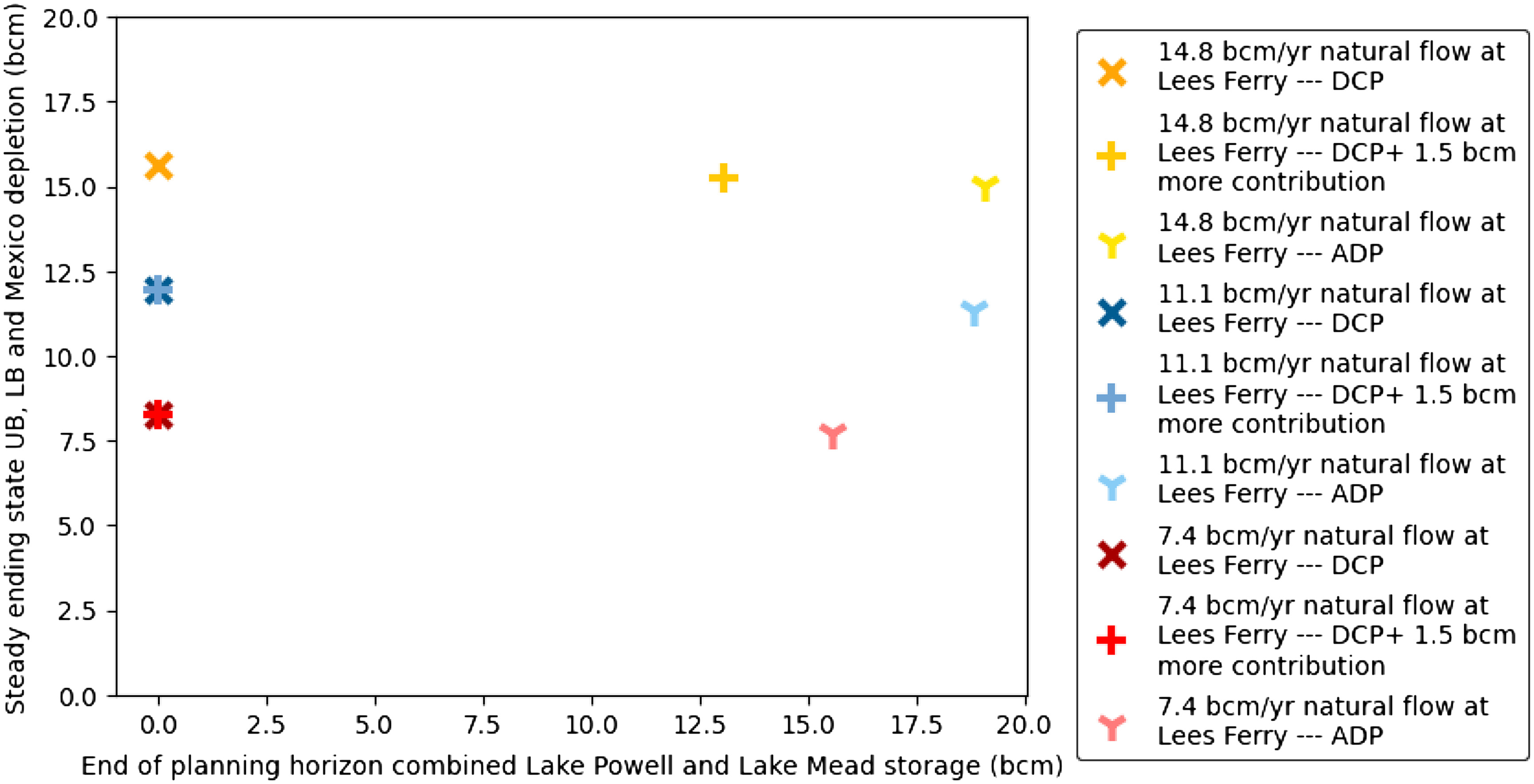
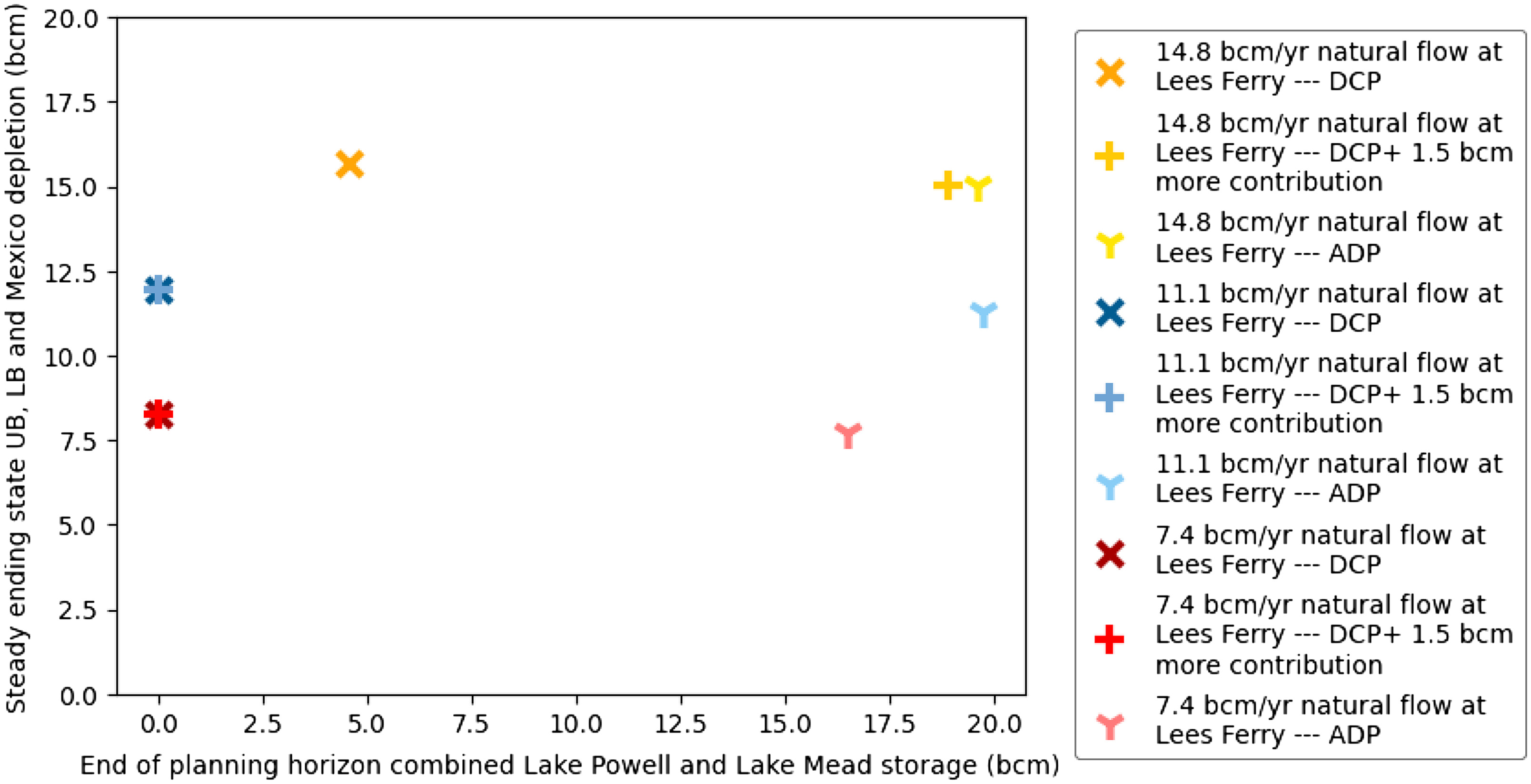
Fig. 5 shows trade-offs between combined reservoir storage volume at the end of the simulation and steady-state basin depletion. The larger the end-of-planning horizon combined storage (which is affected by different policies, indicated by different marker shapes), the smaller are the steady state total depletions under the same amount of natural flow at Lees Ferry (indicated by intensity). Among the three tested policies, DCP emptier reservoir storage first; however, steady-state basin depletion is the largest because reservoir evaporation no longer is a factor after Lake Powell and Lake Mead become run-of-river reservoirs. DCP+ preserves more water than DCP, but only avoids emptying reservoir storage when natural flows were not low. ADP kept the combined reservoir storage higher than 14.8 bcm (12 maf) at the expense of having the lowest steady-state depletion among these policies. However, when combined reservoir storage reaches steady state, only minimal additional cutbacks from ADP are required to keep the reservoirs running above 14.8 bcm (12 maf) compared with DCP or DCP+.
Previous analysis showed that inflow is one dominant factor in declining reservoir storage. Therefore, in addition to reservoir elevation and storage, operating rules for the Colorado River also can consider inflow information because the combined effect of inflow and releases contributes to the changes in reservoir storage. Previous analysis also showed that ADP could keep the combined Lake Powell and Lake Mead storage above 14.8 bcm (12 maf) under different natural flow scenarios at Lees Ferry. This indicates that adapting depletions to inflow is a promising strategy to sustain reservoir storages.
Sharing Shortages
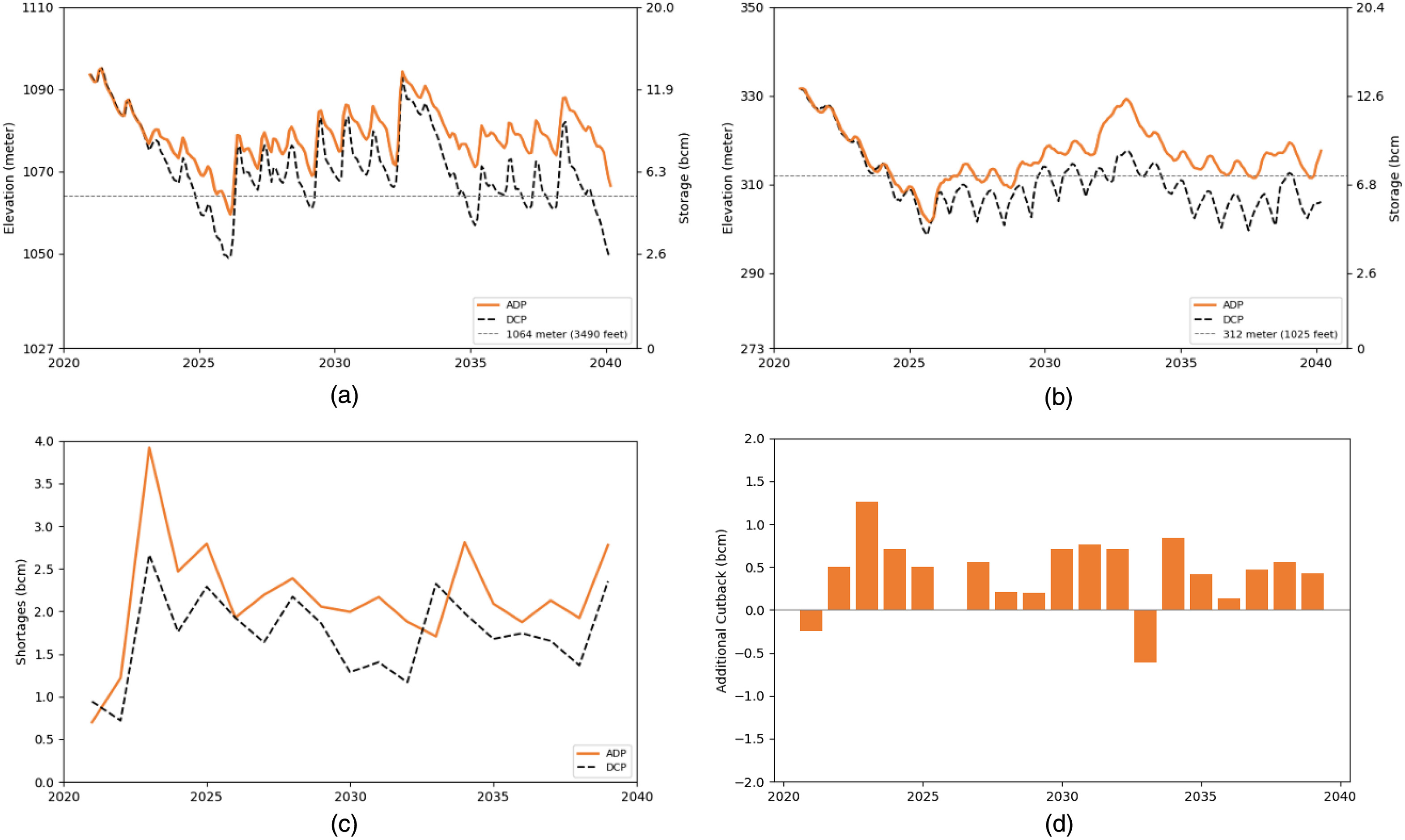
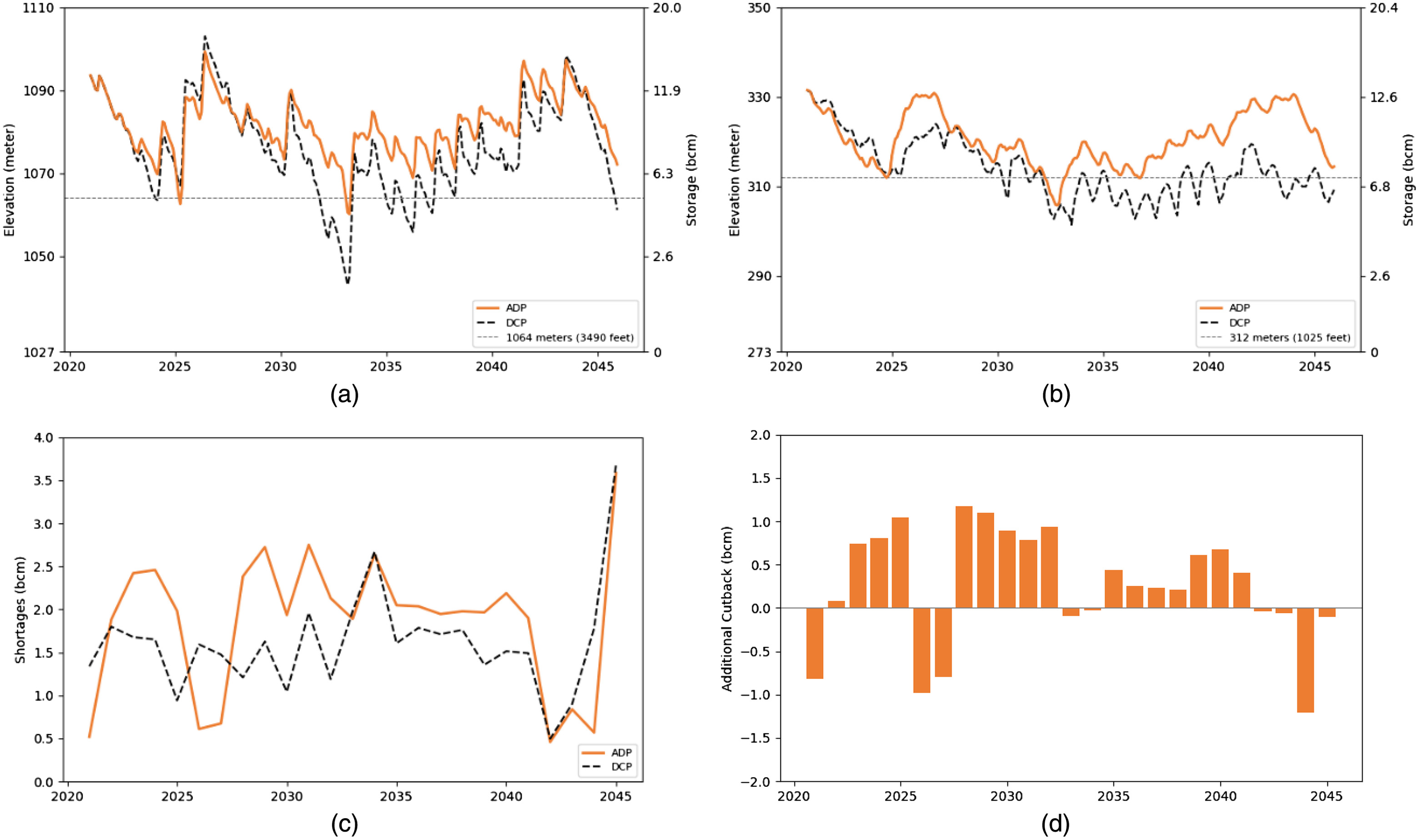
Figs. 6(a and b) compare Lake Powell and Lake Mead elevations for the ADP and DCP policies under the Millennium Drought hydrology [average Lees Ferry natural flow of 15.3 bcm (12.4 maf) per year] (Salehabadi et al. 2020). The ADP policy keeps Lake Powell above 1,064 m (3,490 ft) (the Lake Powell minimum power pool) and Lake Mead above 312 m (1,025 ft) for most of the time [Figs. 6(a and b)], but at the sacrifice of experiencing large water shortages [Figs. 6(c and d)]. The additional water saved by ADP in earlier years is not wasted; instead, some of the water is stored in both Lake Powell and Lake Mead, thus leaving more water for future use. These results demonstrate the value of water conservation. Users get through a hydrologic scenario that continues the Millennium Drought by conserving 0 to 1.2 bcm (1.0 maf) per year [Fig. 6(d)] more than the current DCP. Conserving 1.2 bcm (1.0 maf) more than the current DCP means conserving as much as 0.6 bcm (0.5 maf) per year more than the Lower Basin’s December 2021 conservation pledge of 0.6 bcm (0.5 maf) per year (USBR et al. 2021). Results for the mid-20th century drought (Appendix) were similar, and also highlighted the value of water conservation.
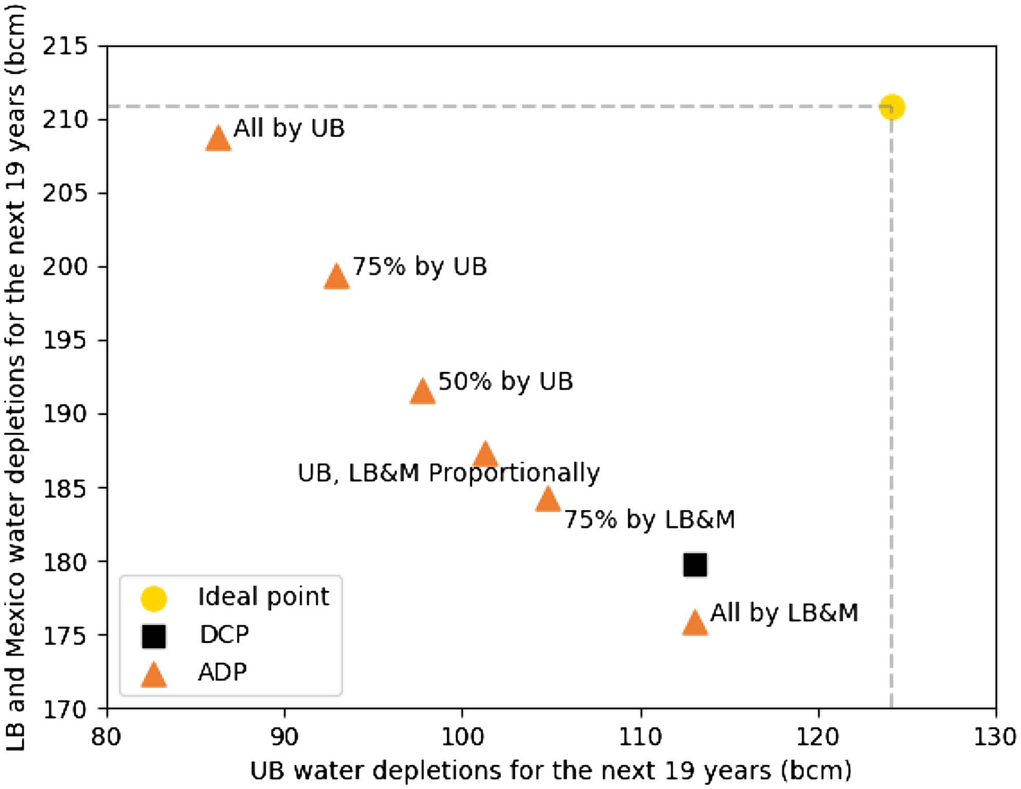
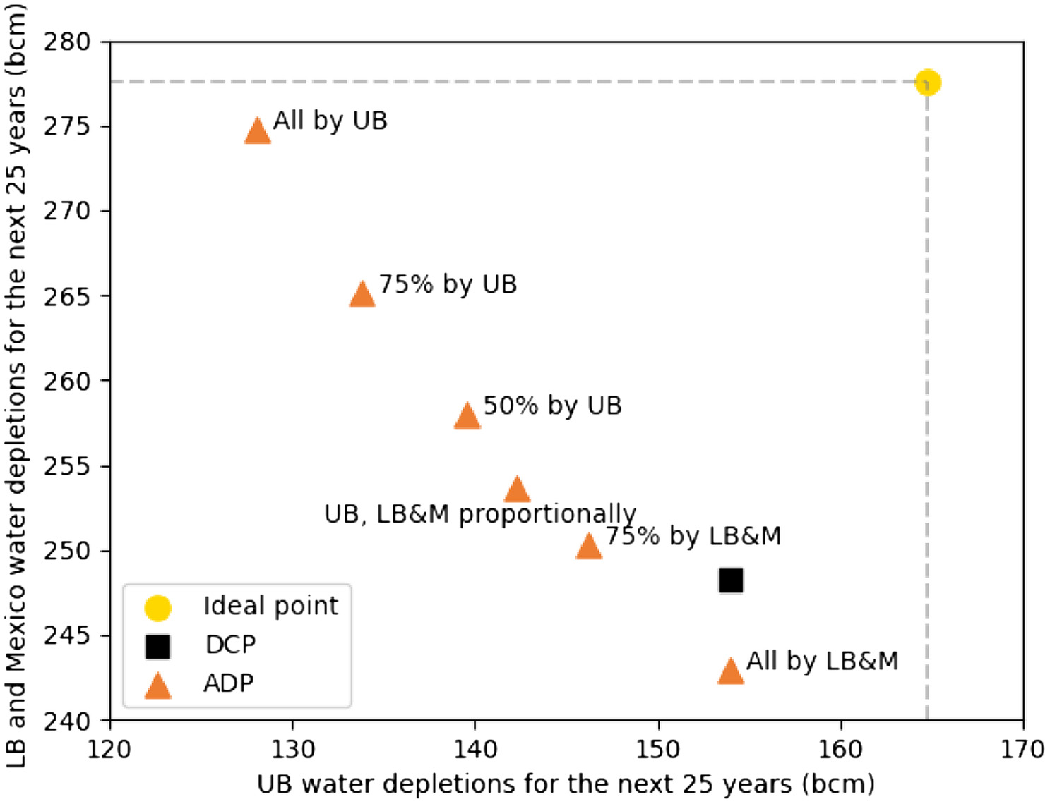
In addition to distributing shortages proportionally to UB and LB and Mexico, we also simulated different allocations of new shortages to the UB and LB and Mexico, and found a quasi-linear tradeoff (Fig. 7). In Fig. 7, the circle represents the complete fulfillment of all demands over the next 19 years. Clearly, the entire basin will not have enough water to satisfy all UB and LB and Mexico demand if the Millennium Drought continues. The quasi-linear tradeoff also indicates that both UB and LB and Mexico contributions are important; no plan is superior to all others. The split of the new shortages should be negotiated by all basin users in a more collaborative way. Results for the mid-20th century drought (Appendix) were similar.
Limitations and Future Works
Numerous adaptive policies exist for reservoir operation. These policies can be triggered by different reservoir storage, inflow, climate, or combinatory triggers. A combined Lake Powell and Lake Mead storage volume also could trigger an adaptive policy. Numerous political choices also shape the selection of a policy and triggers. We simulated one policy that adapted basin depletions to past hydrologic inflows when Lake Mead’s level fell below 323 m (1,060 ft). Future work can test more elevation triggers and incorporate forecast hydrologic information.
The current exploratory model uses aggregated water users and thus could not simulate individual user shortages. Using the aggregated water users may underestimate Upper Basin water shortages when water in Upper Basin tributaries is not sufficient to meet individual user demands but the total streamflow is greater than total Upper Basin demands. Future work can add more tributaries and users to better represent the Colorado River system.
We simulated basin management in monthly time steps, which may not capture important finer time scale river ecosystem responses to daily or hourly streamflow variation. Future work may cross more time scales and consider trade-offs between water volume, hydropower revenue, and ecosystem benefits.
Managers must plan for many possible hydrologic and operational scenarios (Wang et al. 2020). Thus, we made our modeling materials open source so that managers can explore and adjust the model assumptions to see what conservation efforts are required under different hydrologic or operational scenarios in the future.
The adaptive rule to set depletions to inflow also can be implemented in CRSS to provide stakeholders more confidence in results. This implementation will require disaggregating reduced depletions among hundreds of users in the Upper and Lower Basins. Additionally, the adaptive rule will require testing to work with other Lake Powell and Lake Mead rules.
Finally, work is needed to devise conservation programs that adapt and scale to available water. The simulation results can help managers identify conservation targets for different available water scenarios. To encourage their constituents to voluntarily conserve water, managers and authorities can set conservation goals and explain why goals are needed. To incentivize conservation, managers may provide assistance—information, financial, and technical—as well as guidance on water rights. Multiple years of low available water and larger conservation goals pose the extra challenge of helping users sustain and scale their conservation efforts. The Lower Basin’s 0.6 bcm (0.5 maf) per year plan makes a first step to adapting depletions to forecast inflows.
Conclusions
Colorado River reservoirs are drawing down because releases exceed inflows and releases adapt to reservoir elevations instead of elevations and inflow information. To slow reservoir drawdown, this paper introduces a new rule that adapted basin depletions to available water. We validated the existing operations and simulated the adaptive rule in an open-source exploratory model for the Colorado River Basin. Runtime was the CRSS run time in the same single-core computing environment. We simulated adaptive and existing operations for Lees Ferry natural flow scenarios that ranged from 17.3 to 6.2 bcm (14–5 maf) per year. We found that (1) with Lees Ferry natural flow lower than the average 2000–2018 hydrology [15.3 bcm (12.4 maf) per year], the existing rules drew down Lake Powell and Lake Mead to their critical storage levels of 7.4 bcm (6.0 maf) in less than 5 years, and (2) with 2000–2018 hydrology, the adaptive rule sustained both reservoirs above those levels for long periods by requiring Upper and Lower Basin users to conserve as much as 1.2 bcm (1.0 maf) per year more water than operations for the 2019 Drought Contingency Plan. The next steps should be testing the adaptive rule in Reclamation’s Colorado River Simulation System model and devising Upper and Lower Basin conservation programs that can adapt and scale to available water.
Appendix. Supplemental Model Assumptions and Results
Table 2 presents detailed parameters and policies that were used to validate the exploratory model against CRSS. Fig. 8 presents two other typical traces to compare system performance of the exploratory model and CRSS. Results demonstrate the capability of the exploratory model to simulate correctly the two largest reservoirs in the Colorado River system. In addition to using the UCRC UB demand schedule, we also used another relatively smaller UB demand schedule for multidimensional sensitivity analysis (Figs. 9 and 10). Lowering UB demand will delay the reservoir reaching severe conditions and increase end-of-planning horizon storage (Figs. 4 and 5). In addition, Figs. 11 and 12 show how the adaptive policy performs under another severe sustained drought (the mid-20th century drought). The results demonstrate that the ADP is capable of keeping reservoirs running at relatively higher elevations without users losing much water.
| Item | CRSS (August 2020) | Exploratory model |
|---|---|---|
| Planning horizon | 2021–2060 | 2021–2060 |
| Parameters | Initial storage, elevation–volume table, maximum/minimum reservoir elevation, maximum release capacity, minimum release requirement, net periodic parameters for Lake Powell, evaporation rate for Lake Mead, elevation–area table, changing rate of bank storage, and intervening inflows | Initial storage, elevation–volume table, maximum/minimum reservoir elevation, maximum release capacity, minimum release requirement, net periodic parameters for Lake Powell, evaporation rate for Lake Mead, elevation–area table, changing rate of bank storage, and intervening inflows |
| Hydrology | Direct natural flow scenario (113 traces) | Direct natural flow scenario (113 traces) |
| Lake Powell policies | Compute 602a storage | N/A |
| Compute 70R assurance level surplus volume | N/A | |
| End of water year (EOWY) storage forecasts | N/A | |
| Estimate Upper Basin storage | N/A | |
| Powell operations rule | Powell operations rule | |
| Powell spike flow rule | N/A | |
| Powell smooth July operation rule | N/A | |
| Powell limit outflow rule | N/A | |
| Meet Powell min objective release | Meet Powell min objective release | |
| Lower elevation balancing tier | Lower elevation balancing tier | |
| Mid elevation release tier | Mid elevation release tier | |
| Upper elevation balancing tier April–September | Upper elevation balancing tier April–September | |
| Upper elevation balancing tier January–March | Upper elevation balancing tier January–March | |
| Equalization tier | Equalization tier | |
| Add carryover equalization release | N/A | |
| Check bypass capacity | N/A | |
| Lake Mead policies | Set Mead outflow for demands | Set Mead outflow for demands |
| Mead flood control | N/A | |
| Set Mead outflow during extreme low stochastic | N/A |
Data Availability Statement
All data, codes, and models used in this study are available in reference Wang (2022).
Reproducible Results
Mahmudur Rahman Aveek (Utah State University) downloaded, installed, and ran the exploratory model and reproduced the results in all figures.
Acknowledgments
This material is based upon work supported by the US Geological Survey under Grant/Cooperative Agreement No. G16AP00086 Project ID 2020UT303b, the Center for Colorado River Studies at Utah State University, the Catena Foundation, and the Walton Family Foundation. This work benefited from discussions with one Upper and one Lower Basin manager. We thank Carri Richards for her editing assistance.
References
Brown, C., Y. Ghile, M. Laverty, and K. Li. 2012. “Decision scaling: Linking bottom-up vulnerability analysis with climate projections in the water sector.” Water Resour. Res. 48 (9). https://doi.org/10.1029/2011WR011212.
Díaz-González, L., O. A. Uscanga-Junco, and M. Rosales-Rivera. 2021. “Development and comparison of machine learning models for water multidimensional classification.” J. Hydrol. 598 (Jul): 126234. https://doi.org/10.1016/j.jhydrol.2021.126234.
Dogan, M. S., M. A. Fefer, J. D. Herman, Q. J. Hart, J. R. Merz, J. Medellín-Azuara, and J. R. Lund. 2018. “An open-source Python implementation of California’s hydroeconomic optimization model.” Environ. Modell. Software 108 (Oct): 8–13. https://doi.org/10.1016/j.envsoft.2018.07.002.
Draper, A. J., M. W. Jenkins, K. W. Kirby, J. R. Lund, and R. E. Howitt. 2003. “Economic-engineering optimization for California water management.” J. Water Resour. Plann. Manage. 129 (3): 155–164. https://doi.org/10.1061/(ASCE)0733-9496(2003)129:3(155).
Fleck, J. 2020. “How big was Lake Mead’s ‘structural deficit’.” Accessed January 6, 2020. http://www.inkstain.net/fleck/2020/01/how-big-was-lake-meads-structural-deficit-in-2019/.
Haasnoot, M., J. H. Kwakkel, W. E. Walker, and J. ter Maat. 2013. “Dynamic adaptive policy pathways: A method for crafting robust decisions for a deeply uncertain world.” Global Environ. Change 23 (2): 485–498. https://doi.org/10.1016/j.gloenvcha.2012.12.006.
Herman, J. D., J. D. Quinn, S. Steinschneider, M. Giuliani, and S. Fletcher. 2020. “Climate adaptation as a control problem: Review and perspectives on dynamic water resources planning under uncertainty.” Water Resour. Res. 56 (2): e24389. https://doi.org/10.1029/2019WR025502.
Hoerling, M., J. Barsugli, B. Livneh, J. Eischeid, X. Quan, and A. Badger. 2019. “Causes for the century-long decline in Colorado River flow.” J. Clim. 32 (23): 8181–8203. https://doi.org/10.1175/JCLI-D-19-0207.1.
Hundley, N., Jr. 1975. Water and the West: The Colorado River compact and the politics of water in the American West. Berkeley, CA: University of California Press.
International Boundary and Water Commission. 2012. “Minute No. 319: Interim international cooperative measures in the Colorado River Basin through 2017 and Extension of Minute 318 cooperative measures to address the continued effects of the April 2010 Earthquake in the Mexicali Valley, Baja California.” Accessed November 20, 2012. https://www.ibwc.gov/Files/Minutes/Minute_319.pdf.
International Boundary and Water Commission. 2017. “Minute No. 323: Extension of cooperative measures and adoption of a binational water scarcity contingency plan in the Colorado River Basin dated September 21, 2017.” Accessed September 21, 2017. https://www.ibwc.gov/Files/Minutes/Min323.pdf.
Kendall, D. R., and J. A. Dracup. 1991. “A comparison of index-sequential and AR(1) generated hydrologic sequences.” J. Hydrol. 122 (1): 335–352. https://doi.org/10.1016/0022-1694(91)90187-M.
Klipsch, J. D., and T. A. Evans. 2006. “Reservoir operations modeling with HEC-ResSim.” In Vol. 3 of Proc., 3rd Federal Interagency Hydrologic Modeling Conf. Reston, VA: Advisory Committee on Water Information.
Knox, S., P. Meier, J. Yoon, and J. J. Harou. 2018. “A python framework for multi-agent simulation of networked resource systems.” Environ. Modell. Software 103 (Aug): 16–28. https://doi.org/10.1016/j.envsoft.2018.01.019.
Kuhn, E., and J. Fleck. 2019. “Science be dammed: How Ignoring inconvenient science drained the Colorado River.” Accessed November 26, 2019. https://uapress.arizona.edu/book/science-be-dammed.
Milly, P. C. D., and K. A. Dunne. 2020. “Colorado River flow dwindles as warming-driven loss of reflective snow energizes evaporation.” Science 367 (6483): 1252–1255. https://doi.org/10.1126/science.aay9187.
Ouarda, T. B. M. J., J. W. Labadie, and D. G. Fontane. 1997. “Indexed sequential hydrologic modeling for hydropower capacity estimation.” JAWRA J. Am. Water Resour. Assoc. 33 (6): 1337–1349. https://doi.org/10.1111/j.1752-1688.1997.tb03557.x.
Salehabadi, H., D. G. Tarboton, E. Kuhn, B. Udall, K. G. Wheeler, D. E. Rosenberg, S. A. Goeking, and J. C. Schmidt. 2020. “The future hydrology of the Colorado River Basin.” In White paper 4, future of the Colorado River Project, 71. Logan, UT: Utah State Univ.
Smith, J. A., A. A. Cox, M. L. Baeck, L. Yang, and P. Bates. 2018. “Strange floods: The upper tail of flood peaks in the United States.” Water Resour. Res. 54 (9): 6510–6542. https://doi.org/10.1029/2018WR022539.
UCRC (Upper Colorado River Commission). 2007. “Upper Colorado River Division States, current and future depletion demand schedule.” Accessed December 12, 2007. http://www.ucrcommission.com/RepDoc/DepSchedules/Dep_Schedules_2007.pdf.
Udall, B., and J. Overpeck. 2017. “The twenty-first century Colorado River hot drought and implications for the future.” Water Resour. Res. 53 (3): 2404–2418. https://doi.org/10.1002/2016WR019638.
USBR (US Bureau of Reclamation). 2007. “Record of decision: Colorado River interim guidelines for Lower Basin shortages and coordinated operations for Lakes Powell and Mead.” Accessed December 13, 2007. https://www.usbr.gov/lc/region/programs/strategies/RecordofDecision.pdf.
USBR (US Bureau of Reclamation). 2019. “Colorado River Basin Drought Contingency Plans (DCP).” Accessed May 20, 2019. https://www.usbr.gov/dcp/finaldocs.html.
USBR (US Bureau of Reclamation), ADWR (Arizona Department of Water Resources), SNWA (Southern Nevada Water Authority), CAP (Central Arizona Project), and MWD (Metropolitan Water District). 2021. “Press release: Water agencies announce partnership to invest $200 million in conservation efforts to bolster Colorado River’s Lake Mead, under 500+ plan.” Accessed December 15, 2021. https://library.cap-az.com/documents/departments/planning/colorado-river-programs/CAP-500PlusPlan-NewsRelease.pdf.
Wang, J. 2022. “Data to supplement adapting Colorado River Basin depletions to available water to live within our means.” Accessed January 13, 2023. https://www.hydroshare.org/resource/c10a97d775804fbc98f4b95047aa6c95.
Wang, J., D. E. Rosenberg, K. G. Wheeler, and J. C. Schmidt. 2020. Managing the Colorado River for an uncertain future, 30. Logan, UT: Utah State Univ.
Wang, J., and J. C. Schmidt. 2020. Stream flow and losses of the Colorado River in the Southern Colorado plateau, 26. Logan, UT: Utah State Univ.
Wheeler, K. G., D. E. Rosenberg, and J. C. Schmidt. 2019. “Water resource modeling of the Colorado River: Present and future strategies.” In White paper 2, future of the Colorado River project. Logan, UT: Utah State Univ.
Woodhouse, C. A., G. T. Pederson, K. Morino, S. A. McAfee, and G. J. McCabe. 2016. “Increasing influence of air temperature on upper Colorado River streamflow.” Geophys. Res. Lett. 43 (5): 2174–2181. https://doi.org/10.1002/2015GL067613.
Xiao, M., B. Udall, and D. P. Lettenmaier. 2018. “On the causes of declining Colorado River streamflows.” Water Resour. Res. 54 (9): 6739–6756. https://doi.org/10.1029/2018WR023153.
Yang, G., B. Zaitchik, H. Badr, and P. Block. 2021. “A Bayesian adaptive reservoir operation framework incorporating streamflow non-stationarity.” J. Hydrol. 594 (Jun): 125959. https://doi.org/10.1016/j.jhydrol.2021.125959.
Zagona, E. A., T. J. Fulp, R. Shane, T. Magee, and H. M. Goranflo. 2001. “RiverWare: A generalized tool for complex reservoir system modeling 1.” JAWRA J. Am. Water Resour. Assoc. 37 (4): 913–929. https://doi.org/10.1111/j.1752-1688.2001.tb05522.x.
Information & Authors
Information
Published In

Journal of Water Resources Planning and Management
Volume 149 • Issue 7 • July 2023
Copyright
This work is made available under the terms of the Creative Commons Attribution 4.0 International license, https://creativecommons.org/licenses/by/4.0/.
History
Received: Sep 14, 2021
Accepted: Feb 21, 2023
Published online: May 10, 2023
Published in print: Jul 1, 2023
Discussion open until: Oct 10, 2023
ASCE Technical Topics:
- Adaptive systems
- Basins
- Bodies of water (by type)
- Engineering fundamentals
- Ferries
- Hydraulic engineering
- Hydraulic structures
- Inflow
- Models (by type)
- Ports and harbors
- Reservoirs
- River engineering
- Rivers and streams
- Simulation models
- Systems engineering
- Systems management
- Water and water resources
- Water conservation
- Water management
- Water policy
Authors
Metrics & Citations
Metrics
Citations
Download citation
If you have the appropriate software installed, you can download article citation data to the citation manager of your choice. Simply select your manager software from the list below and click Download.
Cited by
- James H. Stagge, David E. Rosenberg, Anthony M. Castronova, Avi Ostfeld, Amber Spackman Jones, Journal of Water Resources Planning and Management’s Reproducibility Review Program: Accomplishments, Lessons, and Next Steps, Journal of Water Resources Planning and Management, 10.1061/JWRMD5.WRENG-6559, 150, 8, (2024).
- Hao Wang, Tao Ma, Optimal water resource allocation considering virtual water trade in the Yellow River Basin, Scientific Reports, 10.1038/s41598-023-50319-6, 14, 1, (2024).
- Amy E. East, Gordon E. Grant, A Watershed Moment for Western U.S. Dams, Water Resources Research, 10.1029/2023WR035646, 59, 10, (2023).