Abstract
Practical Applications
Introduction
Materials and Methods
Autoencoders
Adaptive Exponential Weighted Moving Average Chart
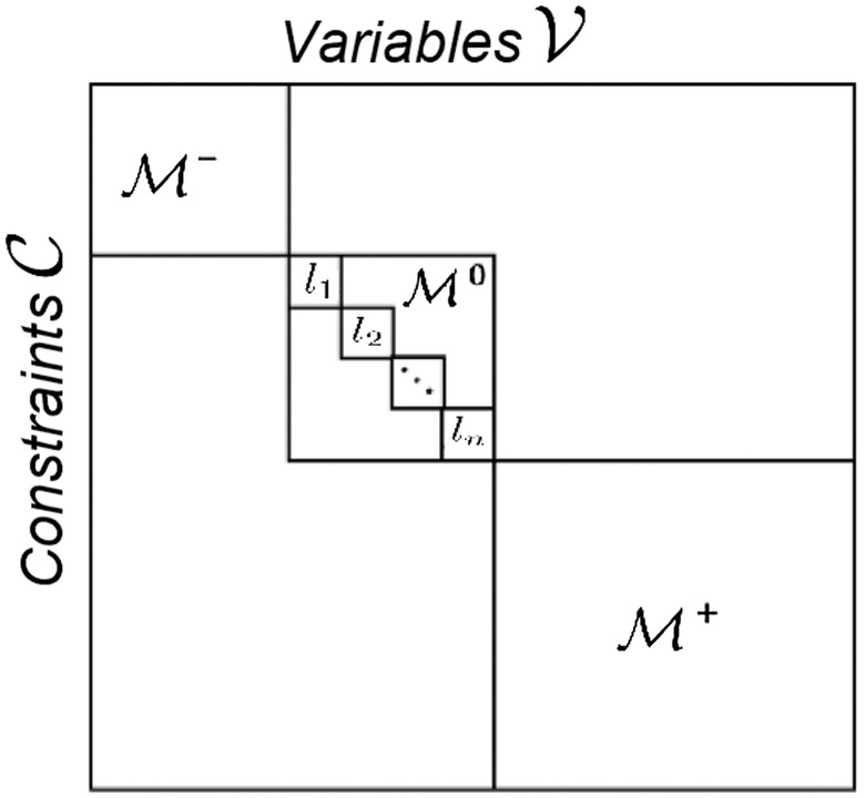
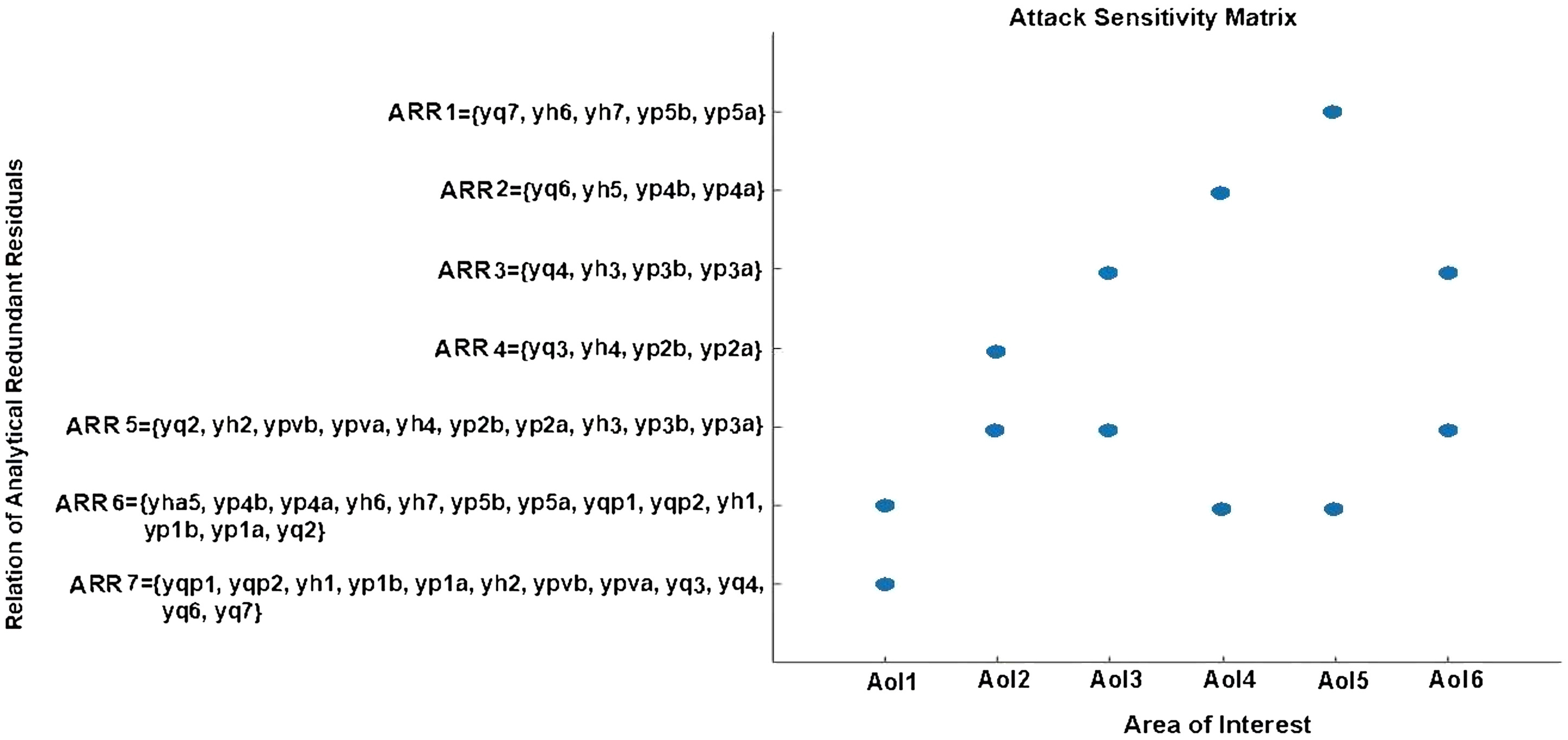
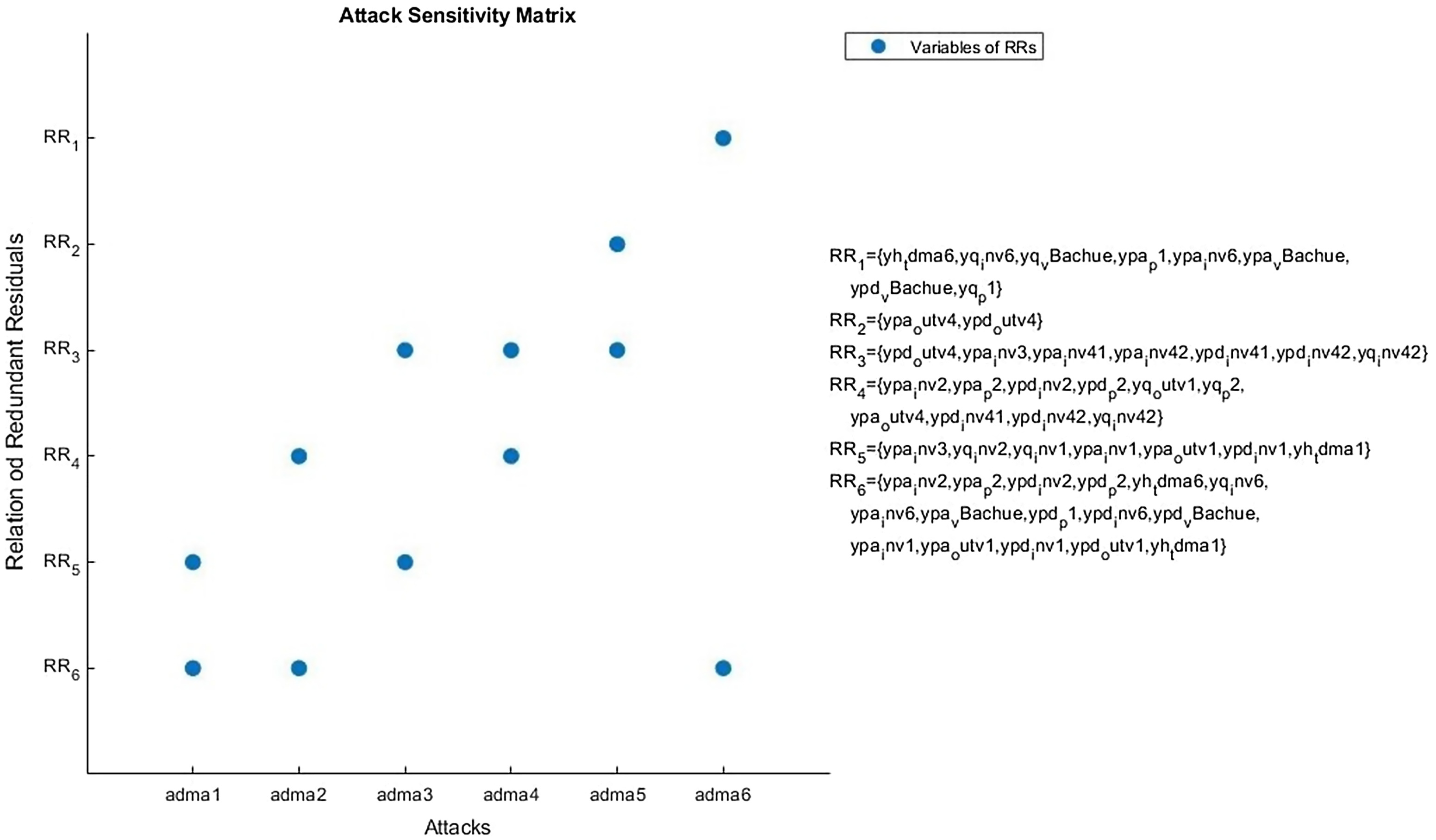
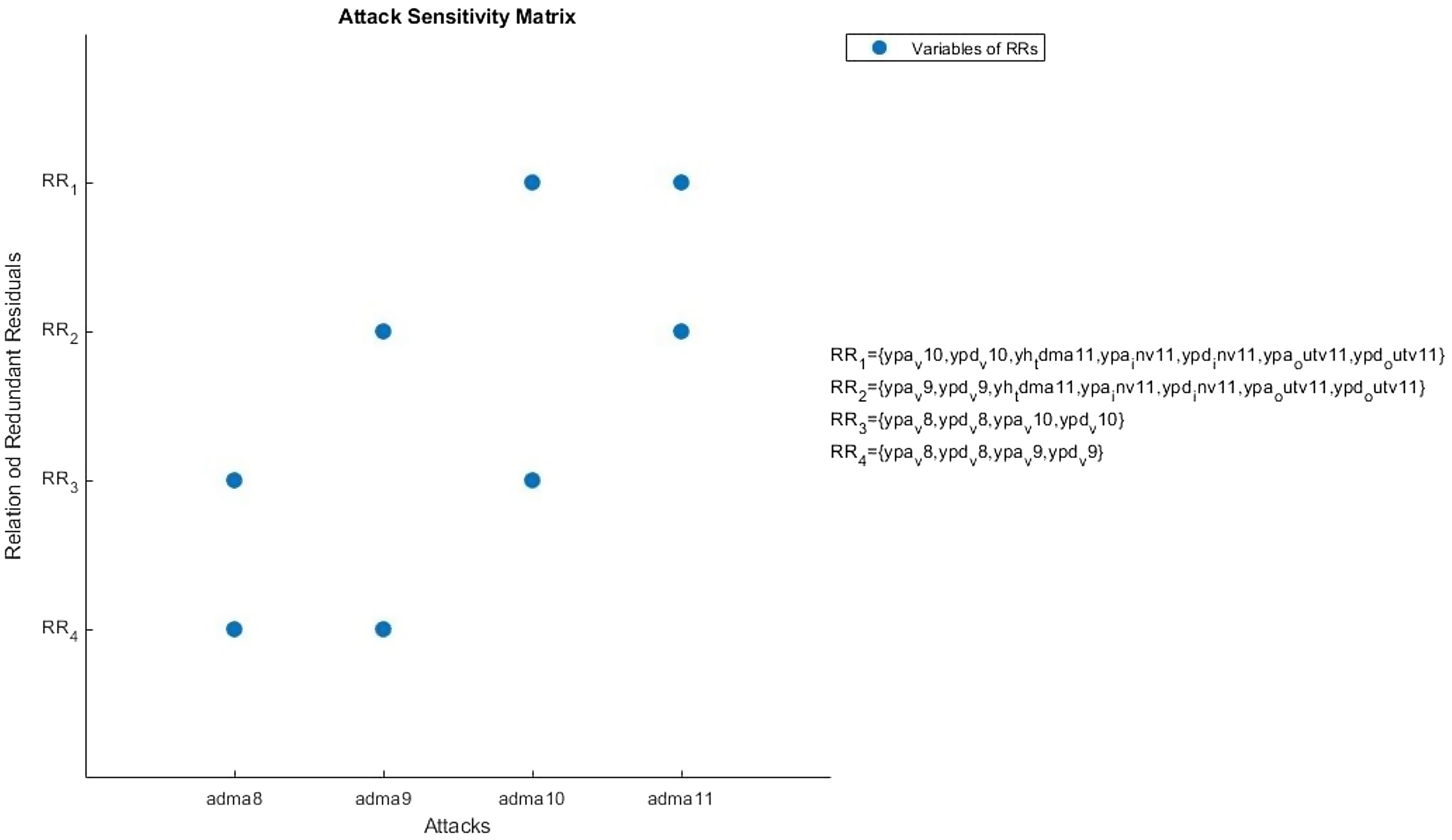
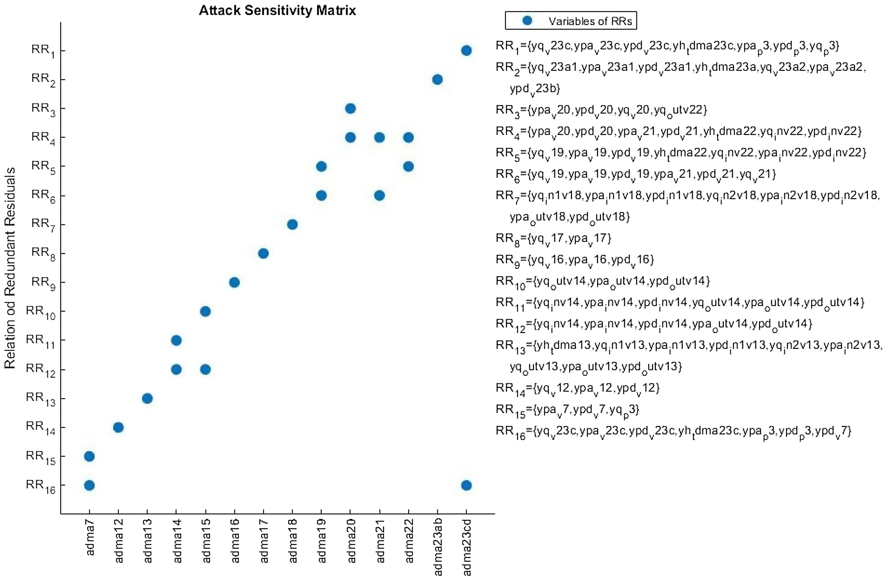
Structural Analysis
Methodology for Detection and Location of Cyberattacks
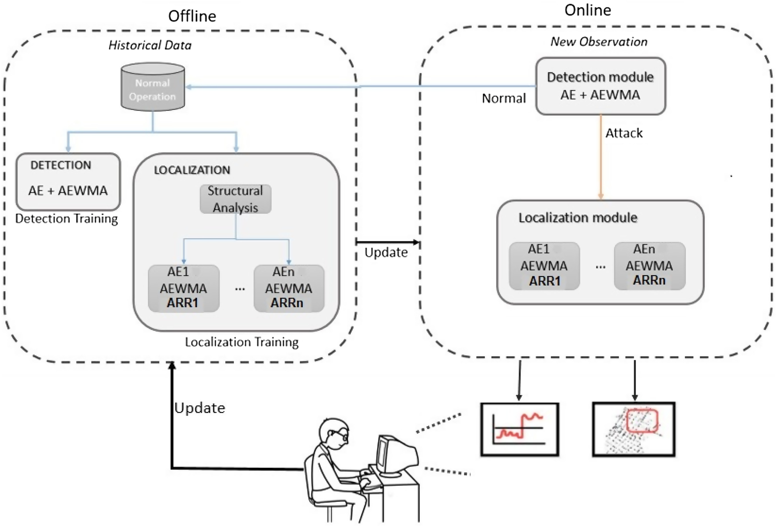
Offline Stage
Online Stage
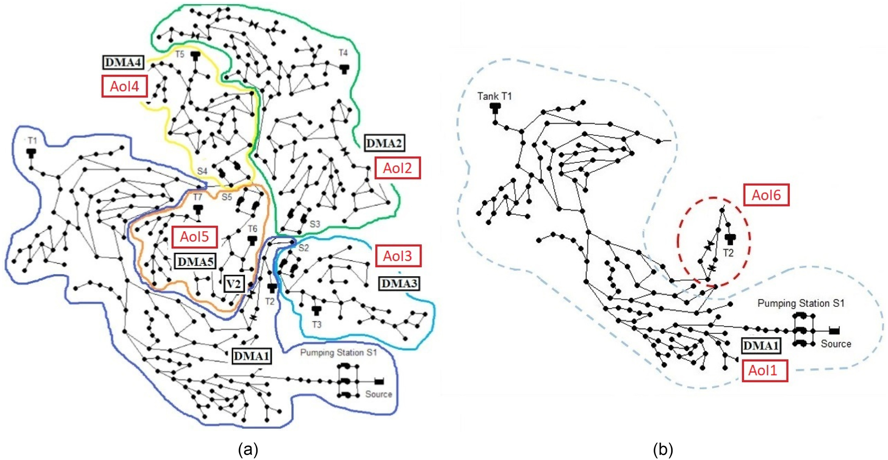
Application of the Proposed Methodology to the C-Town Case Study
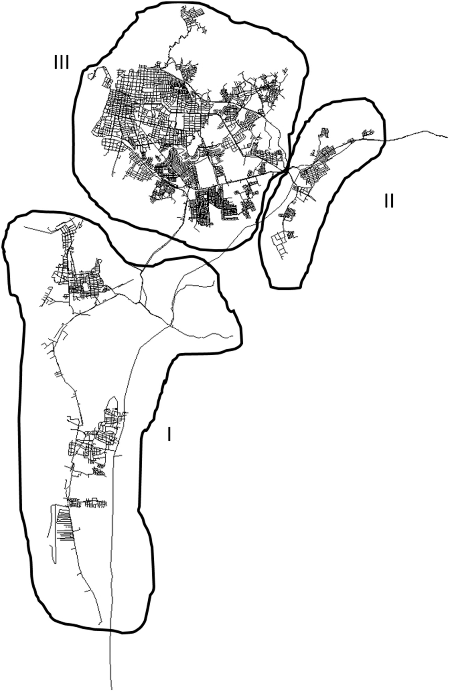
Case Study: C-Town WDN and BATADAL Data Sets
Detection and Localization in the Offline Stage
| Equation No. | Variables involved |
|---|---|
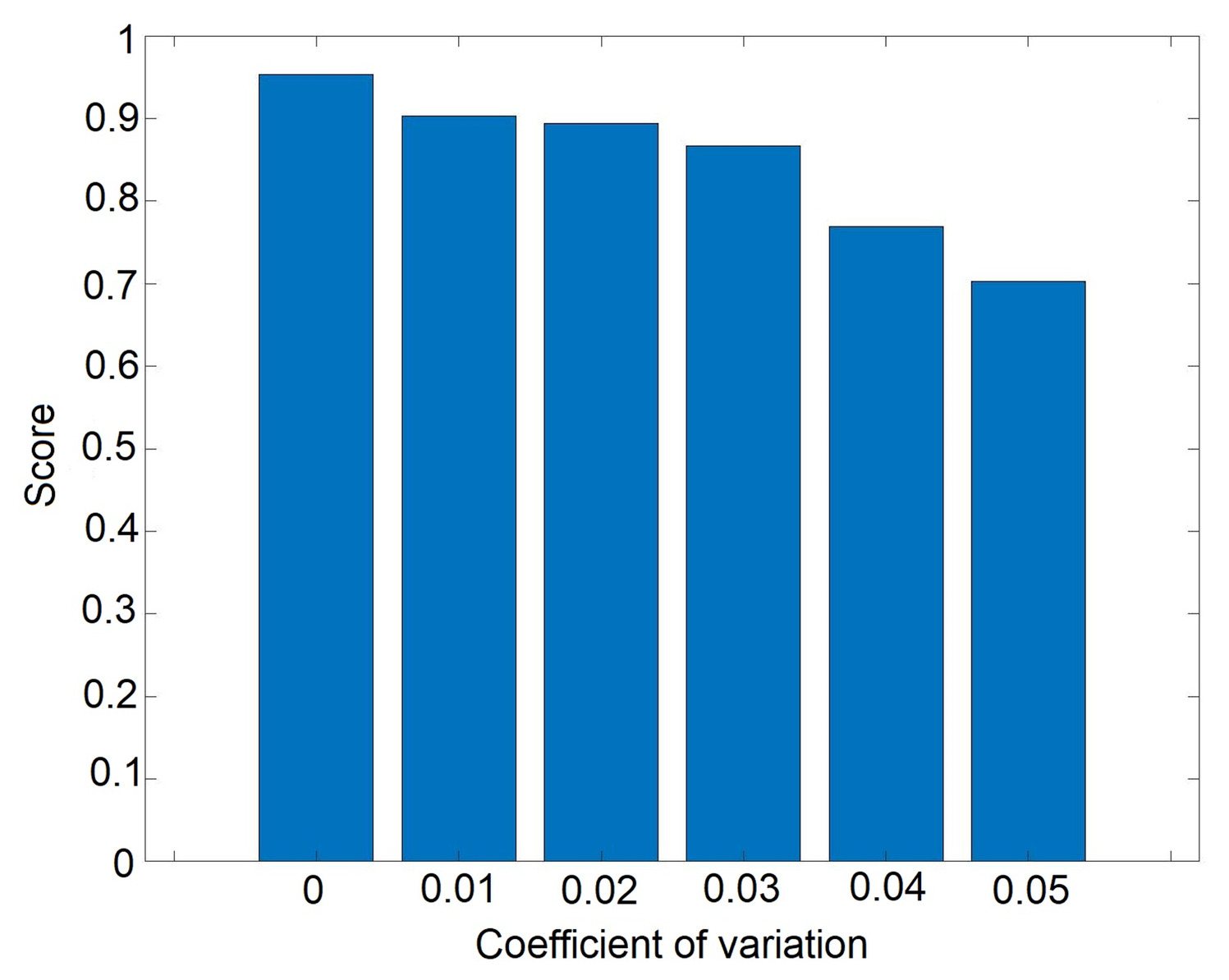
Performance Assessment
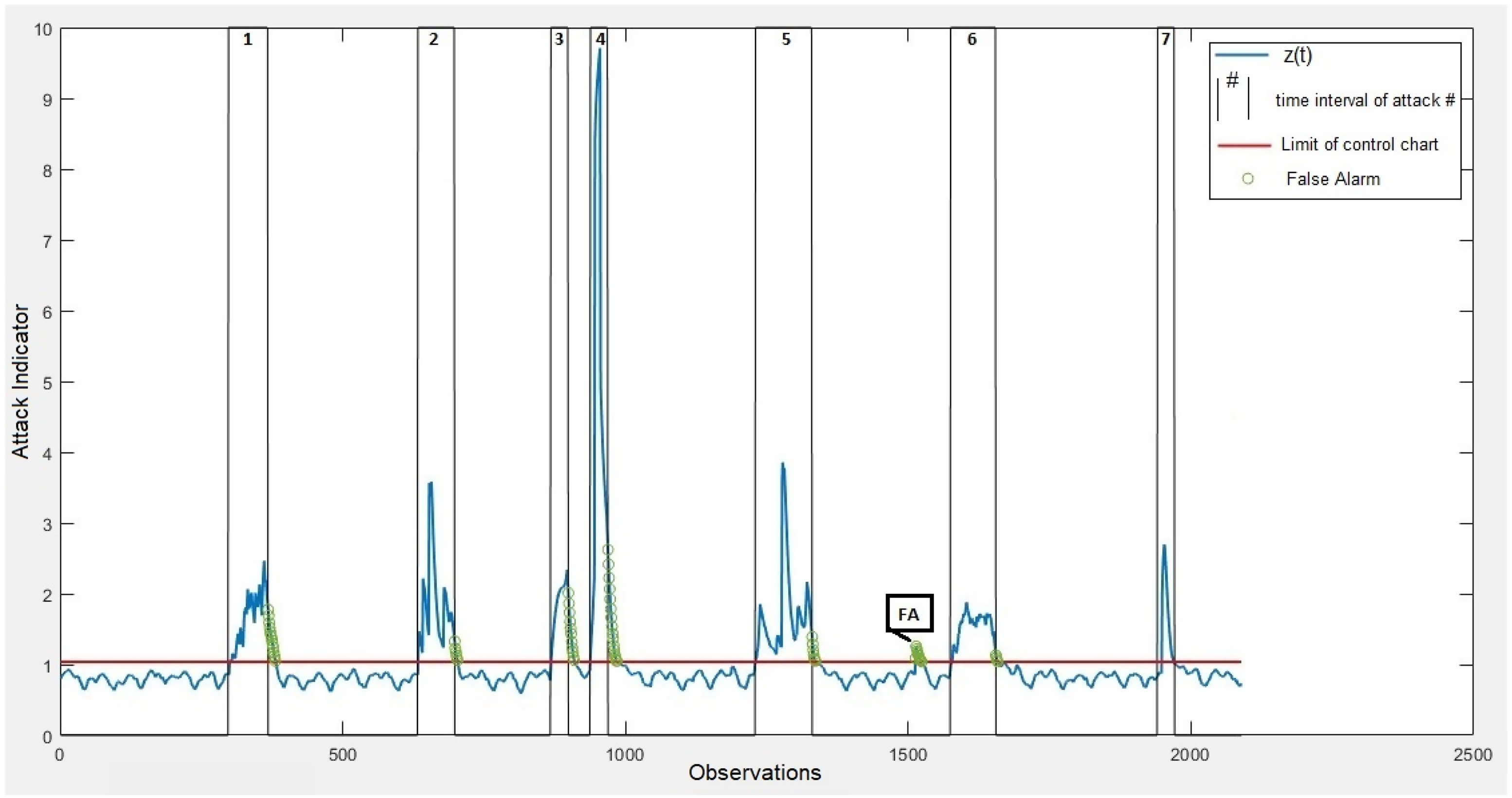
Cyberattack Detection
| Rank | Name | |||
|---|---|---|---|---|
| 1 | B1 | 0.9650 | 0.9752 | 0.9701 |
| 2 | AE-SA | 0.9451 | 0.9583 | 0.9517 |
| 3 | QDA | 0.9584 | 0.9422 | 0.9503 |
| 4 | B2 | 0.9580 | 0.9402 | 0.9491 |
| 5 | Ensemble | 0.9400 | 0.9529 | 0.9464 |
| 6 | MD | 0.9297 | 0.9387 | 0.9342 |
| 7 | B3 | 0.9360 | 0.9174 | 0.9267 |
| 8 | LOF | 0.9229 | 0.9286 | 0.9258 |
| 9 | SOD | 0.9091 | 0.9223 | 0.9157 |
| 10 | B4 | 0.8570 | 0.9313 | 0.8942 |
| 11 | B5 | 0.8350 | 0.7679 | 0.8015 |
| 12 | LDA | 0.7959 | 0.7532 | 0.7745 |
| 13 | B6 | 0.8850 | 0.6605 | 0.7727 |
| 14 | OSVM | 0.7383 | 0.8060 | 0.7721 |
| 15 | B7 | 0.4290 | 0.6398 | 0.5344 |
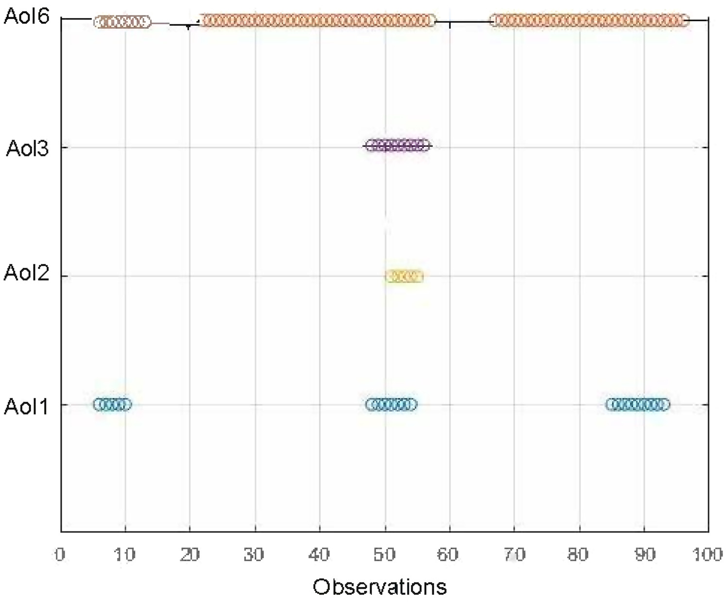
Cyberattack Location
| Attack No. | Elements affected | AOI number |
|---|---|---|
| 1 | Level of Tank 3 (h3), Flow of Pumps 4 and 5 (q4) | 3 |
| 2 | Level of Tank 2 (h2), Flow of Valve 2 (q2) | 6 |
| 3 | Flow of Pump 3 (qp2) | 1 |
| 4 | Flow of Pump 3 (qp2) | 1 |
| 5 | Level of Tank 2 (h2), Flow of Valve 2 (q2), Pressure in Valve 2 (pv) | 6 |
| 6 | Level of Tank 7 (h7), Flow in Pumps 10 and 11 (q7) | 5 |
| 7 | Level of Tank 6 (h6) | 2 |
| A | B | C | D | E | F | G | |||
|---|---|---|---|---|---|---|---|---|---|
| 1 | 70 | 44 | 41 | 3 | 0 | 26 | 62.85 | 93.18 | 100 |
| 2 | 65 | 48 | 41 | 7 | 0 | 17 | 73.84 | 85.41 | 100 |
| 3 | 31 | 29 | 29 | 0 | 0 | 2 | 93.54 | 100 | 100 |
| 4 | 31 | 31 | 29 | 2 | 0 | 0 | 100 | 93.54 | 100 |
| 5 | 100 | 74 | 51 | 23 | 0 | 26 | 74 | 68.91 | 100 |
| 6 | 80 | 23 | 19 | 4 | 0 | 57 | 28.75 | 82.60 | 100 |
| 7 | 30 | 16 | 16 | 0 | 0 | 14 | 53.33 | 100 | 100 |
| Total | 407 | 265 | 226 | 39 | 0 | 142 | 65.11 | 85.28 | 100 |
Note: A = attack number; B = number of observations during each attack; C = number of observations that activate at least one AOI; D = number of observations that satisfy Option 1; E = number of observations that satisfy Option 2; F = number of observations that satisfy Option 3; G = number of observations that satisfy Option 4; LR = location rate, i.e., percentage of observations that activate at least one AOI with respect to total number of observations during an attack []; ExLR = exact location rate, i.e., percentage of observations that activate only the real AOI with respect to number of observations that activate at least one AOI during an attack []; and EfLR = effective location rate [percentage of observations that activate the real AOI with respect to the number of observations that activate at least one AOI [].
Application of the Proposed Methodology to the E-Town Case Study
Case Study: E-Town WDN and Attack Data Set
Detection and Location in the Offline Stage
Cyberattack Detection and Location
| A | B | C | D | E | F | G | |||
|---|---|---|---|---|---|---|---|---|---|
| 1 | 31 | 30 | 30 | 0 | 0 | 1 | 96.77 | 100 | 100 |
| 2 | 41 | 39 | 39 | 0 | 0 | 2 | 95.12 | 100 | 100 |
| 3 | 101 | 100 | 93 | 7 | 0 | 1 | 92.80 | 93 | 100 |
| 4 | 101 | 98 | 98 | 0 | 0 | 3 | 97.03 | 100 | 100 |
| 5 | 101 | 89 | 13 | 76 | 0 | 12 | 88.12 | 14.61 | 100 |
| 6 | 101 | 89 | 0 | 76 | 0 | 12 | 88.12 | 0 | 85.39 |
| 7 | 101 | 97 | 61 | 36 | 0 | 4 | 96.04 | 62.89 | 100 |
| 8 | 101 | 101 | 0 | 79 | 0 | 0 | 100 | 0 | 78.22 |
| 9 | 101 | 101 | 53 | 48 | 0 | 0 | 100 | 52.48 | 100 |
| 10 | 51 | 49 | 49 | 0 | 0 | 2 | 96.08 | 100 | 100 |
| 11 | 101 | 95 | 21 | 64 | 0 | 6 | 94.06 | 22.11 | 89.47 |
| 12 | 51 | 49 | 48 | 0 | 0 | 2 | 96.08 | 97.96 | 97.96 |
| 13 | 21 | 16 | 13 | 2 | 0 | 5 | 76.19 | 81.25 | 93.75 |
| 14 | 151 | 148 | 147 | 0 | 0 | 3 | 98.013 | 99.32 | 99.32 |
| 15 | 51 | 49 | 49 | 0 | 0 | 2 | 96.08 | 100 | 100 |
| 16 | 51 | 51 | 50 | 0 | 0 | 0 | 100 | 98.04 | 98.04 |
| 17 | 151 | 137 | 11 | 83 | 0 | 14 | 90.73 | 8.03 | 68.61 |
| 18 | 71 | 67 | 43 | 22 | 0 | 4 | 94.37 | 64.18 | 97.02 |
| 19 | 81 | 79 | 0 | 79 | 0 | 2 | 97.53 | 0 | 100 |
| 20 | 91 | 89 | 0 | 89 | 0 | 2 | 97.80 | 0 | 100 |
| Total | 1,650 | 1,573 | 818 | 661 | 0 | 77 | 95.33 | 52.00 | 94.02 |
Note: A = attack number; B = number of observations during each attack; C = number of observations that activate at least one AOI; D = number of observations that satisfy Option 1; E = number of observations that satisfy Option 2; F = number of observations that satisfy Option 3; G = number of observations that satisfy Option 4; LR = location rate, i.e., percentage of observations that activate at least one AOI with respect to total number of observations during an attack []; ExLR = exact location rate, i.e., percentage of observations that activate only the real AOI with respect to number of observations that activate at least one AOI during an attack []; and EfLR = effective location rate, i.e., percentage of observations that activate the real AOI with respect to the number of observations that activate at least one AOI [].
Conclusions
Appendix. Structural Analysis Variables
| Structural analysis variable | Description | BATADAL variable |
|---|---|---|
| p1a | Pressure before inlet pumps to DMA 1 | P1 (J820) |
| p1d | Pressure after inlet pumps to DMA 1 | P2 (J269) |
| p2a | Pressure before inlet pumps to DMA 2 | P5(J289) |
| p2d | Pressure after inlet pumps to DMA 2 | P6(J415) |
| p3a | Pressure before inlet pumps to DMA 3 | P3(J300) |
| p3d | Pressure after inlet pumps to DMA 3 | P4(J256) |
| p4a | Pressure before inlet pumps to DMA 4 | P8(302) |
| p4d | Pressure after inlet pumps to DMA 4 | P9(206) |
| p5a | Pressure before inlet pumps to DMA 5 | P10(207) |
| p5d | Pressure after inlet pumps to DMA 5 | P11(317) |
| pv | Pressure in the valve | PV(J422) |
| h1 | Water level, Tank 1 | L_T1 |
| h2 | Water level, Tank 2 | L_T2 |
| h3 | Water level, Tank 3 | L_T3 |
| h4 | Water level, Tank 4 | L_T4 |
| h5 | Water level, Tank 5 | L_T5 |
| h6 | Water level, Tank 6 | L_T6 |
| h7 | Water level, Tank 7 | L_T7 |
| qp1 | Flow through Pump PU1 | F_PU1 |
| qp2 | Flow through Pump PU2 | F_PU2 |
| q1 | Flow through Node J269 | — |
| q2 | Flow that passes through Valve 2 and influences the level in Tank 1 | F_V2 |
| q3 | Flow through Pumps 6 and 7 (Pumps 6 and 7 alternate: when one is on, the other one is off), and this influences the level in Tank 4 | F_PU6 + F_PU7 |
| q4 | Flow through Pumps 4 and 5 (Pumps 4 and 6 alternate: when one is on, the other one is off), and this influences the level in Tank 3 | F_PP4 + F_PU5 |
| q5 | Flow that feeds Flows 6 and 7 | — |
| q6 | Flow through Pumps 8 and 9 (pumps 8 and 9 alternate: when one is on, the other one is off), and this influences the level in Tank 5 | F_PU8 + F_PU9 |
| q7 | Flow passing through Pumps 10 and 11 (Pumps 10 and 11 alternate: when one is on, the other one is off), and this influences the level of Tanks 6 and 7 | F_PU10 + F_PU11 |
| pva | Pressure before the valve | — |
| pvd | Pressure after the valve | — |
| qtn | Flow out of tank , where , 2, 3, 4, 5, 6, 7. | — |
| Attack on Area of Interest , where , 2, 3, 4, 5, 6 | — |
Data Availability Statement
Reproducible Results
Acknowledgments
References
Information & Authors
Information
Published In

Copyright
History
Authors
Metrics & Citations
Metrics
Citations
Download citation
Cited by
- James H. Stagge, David E. Rosenberg, Anthony M. Castronova, Avi Ostfeld, Amber Spackman Jones, Journal of Water Resources Planning and Management’s Reproducibility Review Program: Accomplishments, Lessons, and Next Steps, Journal of Water Resources Planning and Management, 10.1061/JWRMD5.WRENG-6559, 150, 8, (2024).