Multiclass Probit-Based Origin–Destination Estimation Using Multiple Data Types
Publication: Journal of Transportation Engineering, Part A: Systems
Volume 144, Issue 6
Abstract
This paper proposes a bilevel optimization model for multiclass origin–destination (O–D) estimation using various types of data. The multiclass character of the model, a new feature and major contribution to the literature, is important because of increasing interest in simultaneous estimation of O–D tables for various classes of trucks and automobiles. The upper-level optimization is used to derive O–D table entries by minimizing the sum of squared differences between observations from different data sources and the predictions of those values. A probit model is assumed in the lower-level stochastic user equilibrium problem for flow prediction. Extensive experiments have been performed on a test network with different types of link count sensors and turning movements. The tests verify the problem formulation and solution algorithm and offer important insights into the multiclass O–D estimation process with the different types of available data. Adding turning movement data can improve O–D estimation by 71%. Furthermore, classification information is interchangeable among different types of sensors.
Introduction
Since the mid-1970s, there has been interest in estimating origin–destination (O–D) matrices from observable network flow data. For the most part, these efforts have focused on creating either a static or a dynamic O–D table for a single vehicle class (automobiles) and have assumed that the only data available are link counts. Because there is a growing interest in truck movements in urban areas, there is a clear need for O–D estimation methods that treat multiple vehicle classes simultaneously. Estimating O–D tables for trucks is of substantial interest to transportation planners because trucks impose different levels of pavement damage than cars, they have different emission characteristics, they have different accident patterns, and they may be subject to different types of flow controls. It is also important to recognize that there are several different size classes of trucks, whose O–D patterns are likely to be different from one another; this emphasizes the need for general multiclass O–D estimation methods.
Modern traffic-sensing technology offers an increasing ability to classify vehicles as they are counted as well as to create data that are more informative than simple link counts, including output from video detectors, GPS-based (Global Positioning System) vehicle location systems, automatic vehicle identification (AVI) systems, etc. Loop detectors buried in the roadway normally collect link counts of total vehicles; however, single-loop detectors, which are ubiquitous, cannot reliably distinguish a truck from a car. These total counts have been considered usable for single-class (automobile) O–D estimation, but the increasing sophistication of traffic sensors supports multiclass O–D estimation; thus, improved methods for using this better data need to be developed.
The purpose of this research is to develop an improved method for multiclass O–D estimation that is designed specifically to accept a variety of data types that are not limited to just link counts. It is also of interest to test the effectiveness of multiclass O–D estimation under conditions of varying amounts and types of available data. To accomplish these goals, the authors have created a bilevel optimization model where the upper level adjusts entries in the O–D tables for multiple vehicle classes simultaneously and the lower level relates the estimated O–D volumes to link and path flows in the network using a probit model of path choice for individual drivers.
The remainder of the paper is organized as follows. The first section reviews previous efforts at truck-only O–D estimation and previous multiclass models. The next section presents the model formulation, including a discussion of how various types of sensor (or other) data may be used for the multiclass O–D estimation; the solution algorithm for the model is also described. In the next section, insights from computational experiments on a small test network under varying conditions of data availability are highlighted. Conclusions and suggestions for future research are presented in the last section.
Truck O–D Estimation and Multiclass Models
A review of the extensive work on O–D estimation for a single vehicle class is outside the scope of this paper, but it is important to relate the current work to some previous multiclass efforts, particularly those oriented toward truck O–D estimation. List and Turnquist (1994, 1995) propose a method for estimating multiclass truck O–D tables using proportional assignment assumptions; they apply their technique in the New York City metropolitan area. The procedure uses various types of data, including several types of vehicle classification counts that different transportation agencies in the New York area have collected for a variety of special purposes. An extended version of this technique (List et al. 2002) has been instituted as a part of the best-practice model for ongoing use in the New York City area.
Al-Battaineh and Kaysi (2007) provide another example of truck flow estimation using a combination of link count data and regional input–output economic data for Ontario. One of the interesting ideas their work represents is that truck movements are connected to economic activity, so regional economic data may be of help in estimating truck flows. This builds on the general concept that link counts of traffic (truck or otherwise) are not the only useful source of data for estimating O–D tables; further, there is value in creating methods that can integrate a wider variety of data types.
A major difficulty with truck-only O–D estimation methods is that they do not account for the interactions of trucks and automobiles in congested networks. A more complete approach would be to simultaneously estimate separate O–D tables for several vehicle classes (i.e., automobiles and various truck size classes), accounting for the different operating characteristics of the various vehicle classes and their interactions in creating equilibrium flows in the network. However, this clearly is a more complex estimation problem than the single-class models and depends on separating some of the observed data (although not necessarily all) by vehicle class.
There has been very limited work done on estimating O–D tables for multiple vehicle classes, but a noteworthy effort of this type is found in Wong et al. (2005). They develop a formulation and solution algorithm for a five-class problem (autos, taxis, buses, light trucks, and large trucks) for use in Hong Kong, assuming that available data are classified link counts and that the network flows satisfy deterministic user equilibrium (DUE) assumptions. Raothanachonkun et al. (2005, 2006) and Ha et al. (2007) also outline multiclass estimation models using varying assumptions regarding the nature of the multiclass network flows; however, they provide few details of model implementation.
Because some newer types of traffic sensors may provide more information than simple link counts, it is important to have a model formulation that can use this information. Most previous O–D estimation efforts either assume a proportional assignment mechanism (especially for trucks) or are based on DUE assumptions. If the underlying assumption of the model is that traffic flows reflect DUE conditions, then path flows for individual O–D pairs are not uniquely identified and data related to path flows are not readily usable in the O–D estimation. However, if it is assumed that the network flows represent stochastic user equilibrium (SUE), then there is a set of identifiable path flows associated with the equilibrium, and the data on path flows becomes of significant value in the O–D estimation process. Furthermore, the SUE assumption allows for errors in perception on the part of drivers as they make route choice decisions, offering a richer view of equilibrium flows in the network. There has been limited work on using a logit-based SUE model in single-class O–D estimation (Maher et al. 2001). Even less attention has been paid to a probit-based model. The underlying assumption of the probit model (that uncertain route characteristics, or drivers’ perceptions of those characteristics, are approximately normal) is intuitively appealing, but the computations required for assigning traffic to a network using probit-based methods are significantly more complex than the computations for a logit-based assignment. The solution method proposed by the authors can solve a real-world-sized problem without computational issues while using a more appealing probit model.
The following section describes a probit-based model for multiclass O–D estimation that is designed to accept multiple types of data, including link counts (aggregated or separated by vehicle class), partial path information (e.g., turning movements or AVI data), and nontraffic data such as truck trip generation based on economic activity.
Model Formulation
Daganzo (1982) showed that the equilibrium conditions for a SUE flow pattern in a network can be written as the following set of nonlinear equations:where = class volume on link ; = class volume for O–D pair ; and = link utilization coefficients (i.e., the fraction of the class O–D volume for pair that appears on link ). These link utilization coefficients are functions of both the vector of costs on the links of the network () and of the O–D volumes themselves (where is the collection of all elements).
(1)
The SUE conditions represented in Eq. (1) can be incorporated into the O–D estimation process in two different ways. One way is to incorporate the conditions directly as constraints into the optimization for determining the O–D elements. Maher et al. (2001) refers to this approach as equilibrium programming [following terminology that Garcia and Zangwill (1981) define]. A second way is to formulate a bilevel model; here, the upper-level problem adjusts the values and the lower-level problem finds link flows, given those values. The bilevel approach is used here.
Under ideal conditions, the link count data will separate each of the defined vehicle classes, and there will be counts available for all of the network links; however, this is unlikely to be the case in practice. The observed values for the link volumes may correspond to aggregations of the defined vehicle classes, and there may not be observations for all of the links. The available observations will be indexed by , and the set of all observed link counts will be indexed as . The count for observation will be denoted as and include vehicles from a set of classes . The relevant link for observation will be denoted as . The observed link count data and the observations’ connection to the O–D tables for individual vehicle classes under the SUE conditions can be written as follows:
(2)
In addition to the link count data, other types of observations like turning movements or partial path movements may also be available to support the O–D estimation process. An assumed form of constraints representing nonlink count data (for an observation indexed by ) can be expressed as follows:where = observed value; and the values = specified coefficients. Constraint Eq. (3) states that some linear combination of elements in the estimated O–D tables (for a subset of vehicle classes denoted and a subset of the O–D pairs in the set ) should sum to an observed value. This is a relatively general form because the set may have any combination of pairs in it; the set may contain one or more vehicle classes. If a prior estimate of the O–D matrix for one or more vehicle classes is available, that information can be used via Eq. (3), but the expression in Eq. (3) admits a much wider variety of data.
(3)
Before proceeding to a discussion of how Eqs. (2) and (3) form the basis for an O–D estimation process, it is worth digressing briefly to a discussion of how various types of sensors can create usable observed values for and .
Sensors, Observations, and Use of Nontraffic Data
A length-based vehicle classification scheme offers one way of separating vehicle classes, but it has limitations. In urban areas, it is useful to separate subclasses of single-unit trucks [e.g., Federal Highway Administration (FHWA) class 5 from heavier trucks of FHWA classes 6 and 7]. However, it is difficult to separate those single-unit classes using length alone. In relatively uncongested conditions, dual-loop detectors can provide useful data on vehicle length, but the error rate on classifications is often quite high. Nihan et al. (2002) report on their experiments showing that approximately 30–40% of trucks are misclassified. In congested conditions, when vehicles may often stop over a detector, the quality of the data degrades considerably. Wei (2011) has recently developed some methods for length-based vehicle classification using loop detector data under stop-and-go traffic conditions, but overall, vehicle classification remains a troublesome issue and is of particular concern with loop detectors on urban streets.
Video data collection and processing is an alternative means of collecting vehicle classification data; it uses both link counts and turning movements at intersections. However, this form of data collection is considerably more expensive than using loop detectors. Turning movements are not usually collected on an ongoing basis as normal traffic data because collecting the data usually requires manual observers (either to record data in the field or to watch video offline). However, these counts are important for optimal signal timing; thus, they may be collected periodically at a given intersection as part of a project to improve signal timing and intersection operation. For normal traffic engineering use, the total counts of vehicles making various turns are the important data, and it is not common to separately collect counts for vehicles in different classifications.
The potential value of turning movements for O–D estimation is that they specify a sequence of links used by a vehicle rather than just counts on individual links; this provides an element of path information. In most previous O–D estimation efforts, the underlying assumption governing vehicle flows on the network is DUE, and path flows are not uniquely identified by the equilibrium conditions, so this type of partial path information has not been of great interest. However, if the underlying flow pattern is assumed to be SUE, there is a set of identifiable path flows associated with the equilibrium, and this connection makes turning movements of significant potential value for the O–D estimation process.
A multiclass O–D estimation process also creates interest in having the turning movements separated by vehicle class. If the turning movement data are collected manually, this is certainly possible even though it is not commonly done. However, because manual data collection is expensive and not done frequently at any given intersection, there is also interest in automated methods of collecting turning movement data with vehicle classification that could be implemented on a continuous basis. Further development of accurate and effective video collection and processing for turning movement data by vehicle class would be a useful endeavor, particularly when combined with a multiclass O–D estimation capability.
Partial path data are sometimes available from special surveys at specific facilities. For example, truck drivers in line at a tollbooth may be asked for their last stop and next stop information. This is done occasionally at locations like the toll bridges crossing the Hudson River into New York City, but collection of data in this way is labor-intensive, expensive, and prone to substantial reporting errors. In urban networks, this type of data can also be collected by video using license plate–matching software—that is, a specific truck may be observed at several points within a network at different times. Partial path information for the truck can be inferred by matching the data collected by different cameras. The origin (or the final destination) of the truck might not be known, but some information about its path through the network can be inferred as well as whether stops within the network (which define destinations and origins of linked trips) are likely to have been made.
An increasing number of trucks have GPS receivers, and many are capable of reporting their location to some central dispatching center on a regular basis. This type of data is not normally available outside the company that operates the trucks, but it is potentially a very rich data source. There has also been interest in using this type of data from automobiles (an increasing proportion of which are equipped with GPS capability) to estimate O–D information for passenger vehicles.
For truck flows, it can also be helpful to use socioeconomic and land use data to estimate truck trip ends (total origins and total destinations by zone). Several types of truck trip generation models are described by the U.S. Federal Highway Administration (FHWA 2007). Although such estimates are not observed data in the usual sense, they may be used to augment data and create useful relationships of the form in Eq. (3) for the O–D estimation process.
Optimization Model
The observed values, regardless of type, must be assumed to contain errors. Thus, there is likely to be no solution that exactly satisfies Eqs. (1)–(3). The present approach is to search for an O–D matrix Q that minimizes a sum of weighted squared errors, as shown in Eq. (4)where the sets and define the observed values ( and ) for the link counts and nonlink data, respectively. The incorporation of the weighting constants and allows for control of the degree to which emphasis is placed on various observations within the observed data. The values of the coefficients are determined by the assignment of the O–D trips for all the vehicle classes to the network to achieve a stochastic equilibrium flow pattern. The multiclass SUE assignment is itself an optimization—a problem that needs to be solved in order to attain the parameters necessary to evaluate the function in Eq. (4). This illustrates the bilevel character of the overall problem. Evaluation of the objective function for the “upper-level” problem in Eq. (4) requires solving the lower-leve” optimization (the multiclass SUE flow problem).
(4)
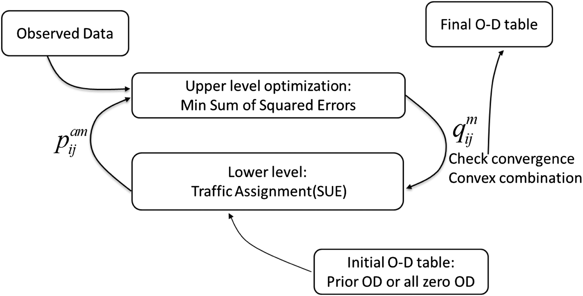
The general flow of information in the solution approach is as follows: a trial solution for the upper-level problem (a set of values) is passed to the lower-level problem (Fig. 1). Assignment of these trips via a multiclass SUE algorithm results in link and path flows and a set of values that are consistent with the input values. These values are passed back to the upper-level problem and treated as constants; the values are adjusted to create a new trial solution to the upper-level problem. If the upper-level problem has converged (i.e., the values are not changing), a solution to Eq. (4) has been reached. However, if the new trial values are different from the previous values, they are passed back to the lower-level problem, where new values are created. In a more formal sense, the algorithm for solving Eq. (4) is as follows:
1.
Set (an iteration counter). When no prior OD table is available, based on free-flow conditions for travel times and costs, compute path flow probabilities for each vehicle class. The result of this loading is a set of values. Denote the collection of values as . For some types of data, the associated values also depend on . Denote the entire collection of values as .
2.
Using the values of from and from (as constants), solve the following problem:
Denote this solution as .
3.
Using the O–D tables for the various vehicle classes, do the SUE calculations to get a feasible solution for the network link volumes, denoted as ; the link utilization values, denoted as ; and the associated data coefficients, denoted as . The collection (, , , ) is termed a consistent solution. (Note that when , the and values computed in this step replace the initial values estimated in Step 1.)
4.
Using the values of from and from (as constants), solve the following problem:
Denote this solution as .
5.
Using the O–D tables for the various vehicle classes, do the SUE calculations to get a feasible solution for the network link volumes, denoted as . This will be termed a trial solution.
6.
Linearize the assignment map between the two feasible solutions so that potential trip tables can be expressed as a function of a step size , where :
7.
Perform a one-dimensional search on to find the following:
The values of and are the values associated with the solution . Denote the optimal value of as .
8.
If the difference is small enough, the solution has converged and the algorithm stops, using the last consistent solution as the final solution. If the process is not converged, make and . Go to Step 3.
The path probability calculations in Steps 1 and 3 of the algorithm require either explicit or implicit path enumeration for each O–D pair. This can be done implicitly using an approach like the stochastic assignment method (SAM) algorithm (Maher 1992), but there is some evidence (Rosa and Maher 2002) that significant errors can be made in estimating path probabilities using the SAM approach. At present, the authors’ interest is in demonstrating proof-of-concept for the model and algorithm, and they have done the path probability calculations using explicit enumeration of efficient paths (Dial 1971) for each O–D pair; they used Mendell and Elston’s method (1974) to calculate probabilities. Although this approach is quite accurate and suitable for small-scale tests, it does not scale well to large networks. Developing a more scalable method for doing the probability calculations is part of the authors’ continuing research efforts.
The optimizations in Steps 2 and 4 of the algorithm are bounded quadratic programming problems. These problems are currently being solved using the limited-memory Broyden-Fletcher-Goldfarb-Shanno with bounds (LBFGS-B) algorithm (Byrd et al. 1995, 1997; Morales and Nocedal 2011). The core of this algorithm is the BFGS, which is a quasi-Newton method for nonlinear optimization. The LBFGS version of this algorithm uses some approximations in the storage of derivatives to create a limited-memory version of the method that is effective for large problems. The further extension to handle simple box constraints on variables (the B suffix) creates an effective method for the problem faced here. The one-dimensional optimization in Step 7 of the algorithm can be done by analytically constructing the derivative of the function by setting it to zero and solving for .
Experiments on a Test Network
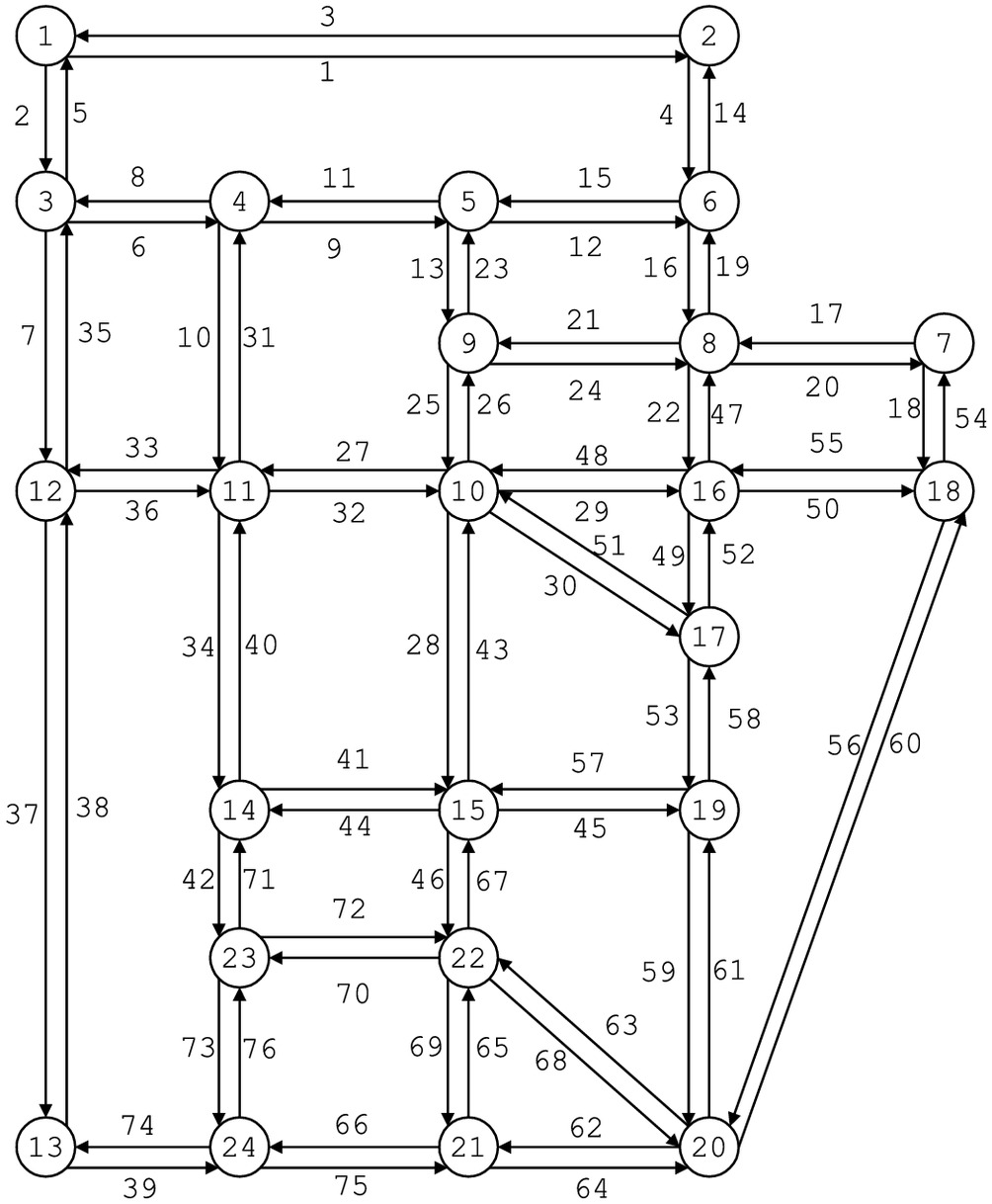
A series of experiments has been developed to test the concepts and solution algorithm. These experiments are designed to test the performance of the solution method under varying conditions and with varying types of data. The tests in this section are performed on a version of the Sioux Falls (SF) network, shown in Fig. 2. This network, first constructed and used by LeBlanc et al. (1975), has since become a standard test network for many types of transportation network algorithms. The basic structure of the network has been retained from the original version used by LeBlanc et al. (1975), but for the current testing, O–D tables and link characteristics have been created that enhance the network’s usefulness as a test bed for the multiclass O–D estimation algorithm. Through SUE calculation, the generated trip table produce link and path flows for each vehicle class. The authors then sample link counts, turning observations at intersections, etc., and create observations that may be separated by vehicle class or aggregated in various ways. This creates a test environment where different sets of assumed data can be specified and the algorithm can be run to estimate multiclass O–D tables. Because the original correct O–D tables are known, the result of various experiments can be evaluated by comparing the estimated tables with the correct tables. The known O–D values are not themselves used as data in any of the tests. The tests are performed using three vehicle classes: automobiles, medium trucks, and large trucks.
To check whether the solution has converged, root mean square (RMS) is used as a criterion. RMS is a statistical measure of the magnitude of a varying quantity. It measures how close the two values or two sets of values are. The calculation of RMS is shown in Eq. (5)where = O–D volume estimated in th iteration for vehicle class m from origin to destination ; and = number of O–D pairs for vehicle class m.
(5)
The termination criteria for the algorithm is set to be maximum 200 iterations or RMS of two successive iterations of O–D volume estimates , whichever comes first. An RMS of 0.1 means on average the squared error of an O–D pair between the two successive iterations is 1%. From experiments performed, most tests converge at approximately 10–30 iterations. If a test does not converge even at 60 iterations, normally it will go all the way until the preset maximum iteration. When this happens, the objective value is normally just bouncing back and forth around the optimum value without much improvement. Therefore setting maximum iteration to 200 should be enough. After the termination criteria are met, the code will output the last set of O–D pairs calculated from the optimization.
RMS can only ensure that the successive two optimization results are close enough. However, it does not necessarily mean that the estimation is close enough to the correct value. The estimation error is computed by the percent difference between the estimated value and true value [Eq. (6)]where = estimated O–D volume for vehicle class m from origin to destination ; = true O–D volume for vehicle class m from origin to destination ; and = estimation error for O–D pair from to for vehicle class m.
(6)
A set of estimation errors can be derived for each test run, one for each O–D pair. An O–D pair is considered as estimated acceptably correctly if the estimation error is within . The percentage of O–D pairs and corresponding volumes estimated correctly for each vehicle class and overall can be used as performance measures to compare the results between different tests.
Basic Tests
Initial tests are performed with a small set of four origin and destination zones (Nodes 1, 7, 15, and 20 in Fig. 2). The assumed O–D tables for the three vehicle classes each contain 12 elements. There are 22,172 total trips in Vehicle Class 1 (automobiles), with individual O–D elements ranging from 839 to 3,117. Vehicle Class 2 (medium trucks) includes 1,498 total trips, with elements ranging from 57 to 215. Vehicle Class 3 (large trucks) includes 1,218 total trips, with elements ranging from 46 to 176.
As a first test of algorithm validity, it is assumed that accurate classified link counts are available for all of the links in the network. In this case, there are 36 unknown O–D volumes to be estimated and 228 observations. This should be sufficient to estimate the O–D tables quite accurately, even though not all of the observations are independent because flow must be conserved at nodes within each vehicle class. In fact, the algorithm estimates 29 of the 36 unknown O–D volumes within 5% of their actual values. The seven O–D volumes outside of the 5% range are small O–D pairs where the estimation errors are small but larger than 5% of the actual volume, with a largest absolute error of 7.3%.
In practice, it is likely that counts will only be available on a modest fraction of links, so a second test assesses the accuracy of the O–D estimates when classified link counts are available to 20% of links (15 links in this test network). Twenty samples of 15 randomly selected links are evaluated. Across those samples, the average number of O–D volumes estimated within 5% of actual values is 14.3. The O–D entries with the largest percentage errors are in vehicle class 2 (medium trucks), where the volumes are relatively small.
It is also likely that in practice not all of the available counts will contain vehicle classification information (in particular, single-loop counters that are widely deployed usually only provide aggregate traffic counts). As a third test, the authors examine how the accuracy of the multiclass O–D estimates is affected when counts are available on all links, but only 25% of the link count sensors can provide classification information. Twenty samples are again evaluated, each corresponding to a random sample of 19 of the 76 sensors that report classification data. On average, 9.6 of the 36 O–D volumes are estimated within 5% of their actual values. The automobile class is more tolerant to the loss of vehicle classification data because most of the vehicles being counted are automobiles, but it is very difficult to estimate truck O–D volumes with any accuracy when a significant fraction of the sensors are only reporting total vehicles counted.
A fourth experiment combines the effects of loss of link coverage and loss of classification information and tests a situation in which 23 of the 76 links have sensors (approximately 30%) but only 11 of them (approximately half) provide classification counts. The remaining sensors only provide total vehicle counts. Again, 20 samples were evaluated. On average, 6.1 of the 36 O–D volumes were estimated within 5% of actual values, and most of those were auto volumes. The effects of losing both link coverage and classification information are quite dramatic.
If vehicle classification data are important but expensive to collect, it is useful to ask whether partial classification data from much cheaper dual-loop detectors would be sufficient. They cannot separate all vehicle classes, but they can distinguish an automobile from a truck. To explore the potential for dual-loop detector data, the authors test a situation where all links have counts and 50% of them are dual-loop detectors. The remaining counts are assumed to be total vehicle counts from single-loop sensors. Across 20 random samples for the dual-loop counter locations, an average of only 8.9 of the 36 O–D volumes are estimated within 5% of actual values, and nearly all are auto volumes. The truck O–D estimation using dual-loop detectors, even with quite extensive deployment, is completely ineffective. If only one aggregate truck class is to be estimated, dual-loop detectors may be acceptable, but counts that cannot distinguish among the different truck classes are almost useless if multiple truck classes are being estimated. Table 1 summarized the tests performed in this section.
| Test case | Purpose | Observations | % OD pairs estimated within 5% of error for Vehicle Class 1, 2, and 3 |
|---|---|---|---|
| 1 | Algorithm validity | Accurate classified link counts on all links | 91.7, 91.7, and 83.3% |
| 2 | Accuracy when limited data available | 20% of links with classified link counts | 36.4% for all vehicle classes |
| 3 | Accuracy when classification information is lost | 25% of links with classified link counters, the rest links are equipped with single-loop detectors only | 33.2, 26.7, and 20.8% |
| 4 | Combination effects of loss of link coverage and loss of classification information | 30% of the links have sensors and half of the sensors provide classification information | 27.5, 11.3, and 14.6% |
| 5 | Effect of dual-loop detector | 50% of the link has dual-loop detectors, the rest of the links are equipped with single-loop counters | 65.0, 1.7, and 1.3% |
Tests with an Expanded Set of O–D Pairs
A second set of O–D tables for the same network contains seven origin and destination zones (Nodes 1, 6, 7, 10, 13, 15, and 20), creating 42 O–D pairs for each vehicle class. The O–D table for Vehicle Class 1 (automobiles) contains 22,084 total trips, with individual elements ranging from 88 to 1,348. In Vehicle Class 2 (medium trucks), there are 1,488 total trips, with entries ranging from 3 to 121. In Vehicle Class 3 (large trucks), there are 1,204 total trips, with entries ranging from 5 to 121.
With this larger set of unknown O–D volumes ( unknowns), link counts alone are insufficient to produce accurate O–D estimates, even with full classification data on all links. Only 35 of the 126 O–D pairs are estimated within 5% of actual values. This result emphasizes the underspecification of the O–D estimation problem when only link counts are used as data.
Under these conditions, it is reasonable to ask whether augmenting the link counts by turning movements at intersections can improve the results. As noted earlier, most of the literature on O–D estimation has paid little attention to turning movements because the partial path information they provide is not important under DUE assumptions, where path flows are not uniquely identified. However, SUE assignments do identify path probabilities, and turning movements may be of greater value. Turning movements are typically collected manually, but surveillance cameras can also provide them; further, there has been some work on reconstructing them from inbound and outbound loop sensors at intersections. As a test of their possible value, the authors add turning movement data from four noncentroid nodes (3, 11, 16, and 22) to the original link count information. These four nodes all have relatively large volumes of traffic.
The authors test three types of turning movement data. Classified turning movements provide counts for all three vehicle classes. Dual-loop turning movements are assumed to be reconstructed from dual-loop counters on entry to and exit from the intersection. These counts differentiate automobiles from trucks, but they group both truck classes together like in the dual-loop link counts. Single-loop vehicle turning movements give only total counts of vehicle movements. In addition, as a base case, the authors include the case where no turning movements are available.
Each type of turning movement count is combined with link counts that include classification information on all links as well as link counts from dual-loop detectors. Table 2 summarizes the results of the experiments using the percentage of O–D pairs that were accurately estimated as a measure. The base case results (no turning movements) are provided for comparison. The availability of turning movements obviously improves the estimation results, and the availability of classified turning movement data at a few busy intersections can further augment dual-loop link count data. It is also worth noting that if the link count data are classified, collecting classified turning movement counts has little advantage over simpler dual-loop turning movement counts. However, it is important to have actual classification counts somewhere—combining dual-loop turning movements with dual-loop link counts is ineffective, especially for estimating truck O–D volumes. Single-loop turning movement counts can improve estimation of automobile O–D volumes if classification counts are available in the link volumes; however, if only dual-loop link counts are available, the total turning volumes do not add any useful information. Single-loop turning movements are not useful for truck O–D estimation under either set of tested circumstances.
| Link count data | Turning movement data | ODs in 5% (%) | ODs in 5% for Class 1 (%) | ODs in 5% for Class 2 (%) | ODs in 5% for Class 3 (%) |
|---|---|---|---|---|---|
| Classified counts | None | 28 | 48 | 17 | 19 |
| Classified | 48 | 62 | 43 | 40 | |
| Dual loop | 35 | 40 | 36 | 29 | |
| Single loop | 34 | 43 | 31 | 29 | |
| Dual loop counts | None | 15 | 29 | 7 | 10 |
| Classified | 25 | 31 | 24 | 19 | |
| Dual loop | 15 | 36 | 5 | 5 | |
| Single loop | 7 | 19 | 2 | 0 |
The previous tests are based on error-free observation; however, in reality, all observations contain errors, and the magnitude of the errors may depend on the type of sensor used. Yi et al. (2010) and Yu et al. (2010) both report errors of 4–10% in classified link counts and turning movements. To test the effects of such errors, the authors conduct an experiment with the case in which link classification counts are augmented by dual-loop turning movement counts at four intersections (no error test case is shown in the third row of Table 2, error test case shown in Table 3). Both types of data are assumed to have 10% errors. The observations are generated through simulation. The error of the sensors is assumed to be the coefficient of variation of a normal distribution, with the mean of the true traffic volume on the link or turning path.
| Error test | ODs in 5% (%) | ODs in 5% for Class 1 (%) | ODs in 5% for Class 2 (%) | ODs in 5% for Class 3 (%) |
|---|---|---|---|---|
| No error | 35 | 40 | 36 | 29 |
| With error | 9 | 10 | 8 | 8 |
A summary of the results is shown in Table 3. There is marked deterioration in the quality of the estimated O–D tables when the observed data contain errors of the magnitude that might normally be expected in practice. This is not unexpected, but these results emphasize two important aspects of the multiclass O–D estimation problem. First, it is important to reduce the errors in the observed data whenever possible. This may mean using better counting technology or doing more filtering of the data before it is used. Second, in the presence of errors, it is necessary to have far more observations to support O–D estimation than would be necessary in an error-free environment. This has implications for sensor location, which includes consideration of both how many sensors to use and where they should be located.
Conclusions and Future Work
The O–D estimation method developed in this research is designed to include multiple vehicle classes whose O–D patterns are different and to accommodate a wider variety of data types than most previous O–D estimation methods, which only rely on link volume counts. This is particularly important for estimating truck O–D matrices along with O–D patterns for auto traffic. It is important to recognize that there are several different size classes of trucks, the O–D patterns of which are likely to be different from one another. There have been several previous efforts to estimate truck O–D matrices independently from automobiles, but the obvious interactions between auto traffic and truck traffic imply that there is a clear need for O–D estimation methods that can treat multiple vehicle classes simultaneously.
For multiclass O–D estimation, it is vital to have data that distinguish among vehicle classes. Modern traffic-sensing technology has an ever-increasing ability to classify vehicles as they are counted as well as to create data that are more informative than simple link counts. The O–D estimation method developed here creates an important new tool for transportation planners who are interested in truck movements (for several size classes) as well as automobile movements and to take advantage of the increasing sophistication of traffic-sensing technology. Use of the SUE assumption for network assignment creates a mechanism for using a wider variety of observed data types that may be related to path flows rather than just link counts. This is an important new capability for taking advantage of increasing sophistication in traffic-sensing technology.
Testing the method developed here on a widely used small test network has verified its ability to successfully estimate O–D tables when sufficient data are available. This has also led to important conclusions about the likely success of multiclass O–D estimation under more typical scenarios of data availability:
1.
Without classified link counts, the estimation of truck O–D volumes is completely ineffective. Even if all sensors can differentiate between automobiles and trucks (i.e., dual-loop counters), the estimates of truck O–D volumes are nearly all incorrect. Using dual-loop detectors to substitute for classification counts in estimating O–D tables with more than one truck class is not likely to prove useful.
2.
Adding turning movement data to link counts is an effective way to increase the quality of O–D estimates; it improved the quality by 71% in the case study. When classification information is not available in the link count data, classified turning movements can dramatically improve estimation of truck O–D tables.
3.
If vehicle classification counts are available from the link data, classified turning movements can be substituted by cheaper dual turning movements and have similar overall O–D estimation accuracy.
4.
There is a marked deterioration in the quality of the estimated O–D tables when the observed data contain errors of the magnitude that might normally be expected in practice. This is not unexpected, but this emphasizes two important aspects of the multiclass O–D estimation problem. First, it is important to reduce the errors in the observed data whenever possible. This may mean using better counting technology or doing more filtering of the data before it is used. Second, in the presence of errors, it is necessary to gather far more observations to support O–D estimation than would be necessary in an error-free environment. This has implications for sensor location, which includes consideration of both how many sensors to use and where they should be located.
Several avenues for further research are suggested. First, additional work to create a more scalable computational process is necessary. The authors have demonstrated proof-of-concept for the multiclass probit-based O–D estimation model, but scaling the computations to large networks remains an ongoing challenge. Second, the experiments done here motivated particular interest in sensor location concerns. That is, with a limited budget for sensor acquisition and deployment, what locations and types of sensors should be selected to maximize the effectiveness of the data for O–D flow estimation across multiple vehicle classes? This sensor location problem is built upon the O–D estimation process developed here by considering the information content of different types of observations.
Extending the methodology to allow dynamic O–D tables is also an important direction. It is clear that both auto flows and truck flows change during the day, and they may change fairly rapidly during certain time periods, such as rush hours. More effective flow control and traffic management across the day, and across different vehicle classes, requires better understanding of the temporal variation of O–D flows. Much progress has been made in recent years in developing dynamic traffic assignment methods for predicting network flows if the O–D flow rates are known. The challenge is to build methods for inferring the O–D flows from these methods and corresponding real-time observations of traffic flows. There are methods focused only on auto traffic, but little has been done in the domain of multiclass dynamic O–D estimation that might apply to both automobiles and trucks.
As more and more types of data becoming available, combine and infer data on emissions and energy consumptions using this model is also an avenue worth pursuing.
Notation
The following symbols are used in this paper:
- index of link;
- relevant link for observation ;
- observed value for nonlink data;
- set of the observed values for nonlink data;
- index of origin node;
- index of destination node;
- index of the available observations;
- set of vehicle classes;
- subset of vehicle classes for observation ;
- index of vehicle class;
- subset of the O–D pairs for observation ;
- number of O–D pairs for vehicle class m;
- probability matrix consisting of the entire collection of values;
- free-flow probabilities matrix;
- link utilization coefficient (i.e., the fraction of the class O–D volume for pair that appears on link );
- O–D matrix consisting of the entire collection of values;
- class volume for O–D pair ;
- estimated O–D volume for vehicle class from origin to destination ;
- O–D volume estimated in nth iteration for vehicle class from origin to destination ;
- coefficient matrix consisting of the entire collection of values;
- specified coefficients;
- trail solution for the network link volumes;
- feasible solution for the network link volumes;
- set of all observed link counts;
- class volume on link ;
- count for observation ;
- trail O–D matrix;
- step size, where ;
- optimal value of ;
- estimation error for O–D pair from to for vehicle class m;
- weighting constant; and
- weighting constant.
Acknowledgments
This research was supported in part by Xerox Corporation and the U.S. Department of Transportation through the Region II University Transportation Research Center. This support is gratefully acknowledged, but the authors are solely responsible for the content and findings of the paper.
References
Al-Battaineh, O., and Kaysi, I. A. (2007). “Genetically-optimized origin-destination estimation (GOODE) model: Application to regional commodity movements in Ontario.” Can. J. Civ. Eng., 34(2), 228–238.
Byrd, R. H., Lu, P., Nocedal, J., and Zhu, C. (1995). “A limited memory algorithm for bound constrained optimization.” SIAM. J. Sci. Comput., 16(5), 1190–1208.
Byrd, R. H., Lu, P., Nocedal, J., and Zhu, C. (1997). “Algorithm 778: L-BFGS-B: Fortran subroutines for large-scale bound-constrained optimization.” ACM. T. Math. Software, 23(4), 550–560.
Daganzo, C. F. (1982). “Unconstrained extremal formulation of some transportation equilibrium problems.” Transp. Sci., 16(3), 332–360.
Dial, R. B. (1971). “A probabilistic multipath traffic assignment algorithm which obviates path enumeration.” Transp. Res., 5(2), 83–111.
FHWA (Federal Highway Administration). (2007). “Quick response freight manual II.”, Washington, DC.
Garcia, C. B., and Zangwill, W. I. (1981). Pathways to solutions, fixed points and equilibria, Prentice-Hall, Englewood Cliffs, NJ.
Ha, T.-J., Lee, S., Kim, J., and Lee, C. (2007). “Gradient method for the estimation of travel demand using traffic counts on a large scale network.” Int. Conf. on Multimedia Modeling, T.-J. Cham, et al., eds., Vol. 4352, Springer, Berlin, 599–605.
LeBlanc, L. J., Morlok, E. K., and Pierskalla, W. (1975). “An efficient approach to solving the road network equilibrium traffic assignment problem.” Transp. Res., 9(5), 309–318.
List, G. F., Konieczny, L. A., Durnford, C. L., and Papayanoulis, V. (2002). “Best-practice truck-flow estimation model for the New York City region.” Transp. Res. Rec., 1790, 97–103.
List, G. F., and Turnquist, M. A. (1994). “Estimating truck travel patterns in urban areas.” Transp. Res. Rec., 1430, 1–9.
List, G. F., and Turnquist, M. A. (1995). “A GIS-based approach for estimating truck flow patterns in urban settings.” J. Adv. Transp., 29(3), 281–298.
Maher, M. J. (1992). “SAM—A stochastic assignment model.” Mathematics in transport planning and control, Oxford University Press, New York, 121–133.
Maher, M. J., Zhang, X., and Van Vliet, D. (2001). “A bi-level programming approach for trip matrix estimation and traffic control problems with stochastic user equilibrium link flows.” Transp. Res., 35B(1), 23–40.
Mendell, N. R., and Elston, R. C. (1974). “Multifactorial qualitative traits: Genetic analysis and prediction of recurrence risks.” Biometrics, 30(1), 41–57.
Morales, J. L., and Nocedal, J. (2011). “Remark on ‘algorithm 778: L-BFGS-B: Fortran subroutines for large-scale bound constrained optimization.’” ACM. T. Math. Software, 23(4), 550–560.
Nihan, N. L., Zhang, X., and Wang, Y. (2002). “Evaluation of dual-loop data accuracy using video ground truth data.”, Univ. of Washington, Seattle.
Raothanachonkun, P., Sano, K., and Matsumoto, S. (2005). “Estimation of multiclass time-varying origin-destination matrices from traffic counts.” Proc. Infrastruct. Plann., 32.
Raothanachonkun, P., Sano, K., and Matsumoto, S. (2006). “Estimation of multiclass origin-destination matrices using genetic algorithm.” Infrastruct. Plann. Rev., 23, 423–432.
Rosa, A., and Maher, M. J. (2002). “Algorithms for solving the probit path-based stochastic user equilibrium traffic assignment problem with one or more user classes.” Proc., 15th Int. Symp. on Transportation and Traffic Theory, Univ. of South Australia, Adelaide.
Wei, H. (2011). “Optimal loop placement and models for length-based vehicle classification and stop-and-go traffic.”, Univ. of Cincinnati, Cincinnati.
Wong, S. C., et al. (2005). “Estimation of multiclass origin-destination matrices from traffic counts.” J. Urban Plann. Dev., 19–29.
Yi, P., Shao, C., and Mao, J. (2010). “Development and preliminary testing of an automatic turning movements identification system.” Ohio Transportation Consortium, Akron, OH.
Yu, X., Prevedouros, P. D., and Sulijoadikusumo, G. (2010). “Evaluation of autoscope, SmartSensor HD, and infra-red traffic logger for vehicle classification.” Transp. Res. Rec., 2160, 77–86.
Information & Authors
Information
Published In

Journal of Transportation Engineering, Part A: Systems
Volume 144 • Issue 6 • June 2018
Copyright
This work is made available under the terms of the Creative Commons Attribution 4.0 International license, http://creativecommons.org/licenses/by/4.0/.
History
Received: Jun 13, 2017
Accepted: Oct 20, 2017
Published online: Mar 27, 2018
Published in print: Jun 1, 2018
Discussion open until: Aug 27, 2018
Authors
Metrics & Citations
Metrics
Citations
Download citation
If you have the appropriate software installed, you can download article citation data to the citation manager of your choice. Simply select your manager software from the list below and click Download.