Resampling Methods in Neural Networks: From Point to Interval Application to Coordinate Transformation
Publication: Journal of Surveying Engineering
Volume 149, Issue 1
Abstract
In the development of neural networks, many realizations are performed to decide which solution provides the smallest prediction error. Due to the inevitable random errors associated with the data and the randomness related to the network (e.g., initialization of the weight and initial conditions linked to the learning procedure), there is usually not an optimal solution. However, we can advantage of the idea of making several realizations based on resampling methods. Resampling methods are often used to replace theoretical assumptions by repeatedly resampling the original data and making inferences from the resampling. Resampling methods provide us the opportunity to do the interval prediction instead of only one point prediction. Following this idea, we introduce three resampling methods in neural networks, namely Delete-d Jackknife Trials, Delete-1 Jackknife Trials, and Hold-Out Trials. They are discussed and applied to a real coordinate transformation problem. Although the Delete-1 Jackknife Trials offer better results, the choice of resampling method will depend on the dimension of the problem at hand.
Introduction
Arising from the field of machine learning, Artificial Neural Networks, also referred to as neural networks, have been used to model the nonlinear relationship between two or more variables and to recognize complex patterns in the data. They provide powerful data analysis tools to handle various types of problems in many fields of engineering sciences, such as:
•
Data Interpolation, such as modeling geoid undulations (Kavzoglu and Saka 2005; Stopar et al. 2006; Lin 2007), determination of the crustal velocity field (Farolfi and Del Ventisette 2016), modeling of tropospheric delay (Yang et al. 2021a);
•
Geodetic Structural Monitoring (Kaloop and Kim 2014);
•
Image Analysis tasks, for example, feature extraction and image classification (Sothe et al. 2020), image detection (Liu et al. 2020), and image recognition (Yang et al. 2021b);
•
Geographic Information System applications (e.g. modeling of spatial pattern (Mollalo et al. 2019); and
•
Coordinate Transformation among different reference systems (Tierra et al. 2008; Ziggah et al. 2016).
One of the most important tasks in developing a neural network is related to partitioning the dataset at hand. Most neural network designers randomly and uniformly split the known dataset into three categories: training, validation, and test. The training set is often used to estimate the unknown parameters of net (e.g., weights in a regression feed-forward neural network). Ultimately, the will have been well learned over its training set. However, a low error in the training set does not tell us much about the quality of the network. What would happen if that trained network was applied to another input dataset? This question is highly relevant. To answer that question, one should use the validation set. The validation set helps one to make decisions on how to train the network and how to stop it to avoid overfitting. However, until now, the total training process of the neural network depends not only on the training set, but also the validation set. It means that any choice regarding training and validation splitting affects the performance of the network. In other words, without the test set we cannot conclude anything about that choice and which choice is good enough in terms of network generalization. In machine learning language, therefore, test sets are unseen data that play an important role in the evaluation of the generalized performance of the network.
This idea of splitting data in a random and uniform way and using the test set to measure the predictive accuracy and stability of the selected trained network model is known as Hold-out cross-validation. There is, however, significant limitations of using this method, as pointed out by Ziggah et al. (2019b) as follows: (1) the results are based on uncontrolled chosen split sets; (2) improper splitting of the data set could have an adverse effect on the model performance; and (3) the results are dependent on the existence of a large dataset making it unsuitable to be applied in data-insufficient situations (i.e., sparse dataset). To overcome these problems, K-fold cross-validation has been recommended as an alternative method (Burman 1989; Reitermanová 2010). In this method, the data is separated into K disjoint subsets (K-fold) of approximately equal size, so that each subset will be in a test set just once. For instance, for each K subset of cross-validation the union of K-1 folds is used as a training set for model development while the remaining part is used as the test set for model validation. Therefore, with this method, the division of data is less of a concern than the case of Hold-out cross-validation, because the entire dataset is employed as both training and testing sets.
The development of a neural network always relies on a certain degree of randomness. In general, the randomness arises in two different parts in neural network modeling: (1) choosing the network architecture, initialization, and learning procedure; and (2) choosing where to split the data (training, validation, and testing sets). There is usually no best choice for this randomness (Pan 1998). However, currently, we have a multitude of neural network models and the continuous development of new architectures to meet different purposes. Consequently, the choice about the network itself is less of a concern than data splitting. Many researchers usually draw many realizations for a given split data set to decide among the different networks which one best suits a certain problem. Although the K-fold presents advantages over the Hold-out cross-validation, it is still not clear on how to choose the K disjoint subsets and in some cases, the subsets are not of equal sizes, which does not guarantee a balanced version of cross-validation. Therefore, splitting data methods are still challenging.
Now the most important question is how to maximize the prediction result since it varies according to the randomness both over data splitting and over the network itself including architecture, initialization, and learning procedures. In light of this issue, we provide a framework that can capture the randomness related to the network itself. To accomplish this, we introduce the resampling methods and apply them in the neural networks context applied to surveying engineering.
The resampling methods replace some theoretical assumptions and derivations by repeatedly resampling the original data and making inferences from the re-sampled data (Efron 1982; Wood 2005). Here, we list the reasons for using resampling methods in real time:
•
Our present-day computers are powerful enough to run resampling algorithm methods.
•
The properties of the original data are preserved. Most resampling methods are based only on the sample of the original data that does not generate additional model errors (Efron 1980).
•
Some resampling methods do not require assumptions and computations of complex formulas related to the distribution of estimators and/or predictors.
•
A closed-form expression of the accuracy measure of a estimator or a predictor can be too complicated or even impossible to obtain. In that case, one can resort to resampling methods.
•
In some situations, the derivative calculation of the nonlinear functions can be discarded by resampling methods.
•
The use of resampling methods can effectively reduce the bias, which can therefore gain more accurate parameter estimates (Wang and Yu 2020).
One of the resampling methods which has been proposed for geodetic data processing is known as Jackknife. This method was developed by Quenouille (1949). Jackknife was initially proposed to estimate the bias of an estimator by iteratively deleting only one single observation each time from the sample, and then recomputing the statistic or estimator on the rest of the sample data. This Jackknife method usually refers to the classic Delete-1 Jackknife estimator. Based on the availability of powerful computers, several researchers have worked to improve the resampling methods, as shown in Tukey (1958), Miller (1974), Efron (1992), McIntosh (2016), Wang et al. (2022), and Wang and Yu (2020, 2021).
In the context of neural networks, the Delete-1 Jackknife method is a balanced version of cross-validation, in which one observation is used to validate the performance of the neural network trained by the remaining () observations. In machine learning language, the Delete-1 Jackknife method is commonly referred to as leave-one-out procedure. The other balanced version of cross-validation is known as the Delete-d Jackknife method, or grouped Jackknife. In that case, instead of validating one observation at a time, we validate the subset of size and train the model with the remaining () observations at a time. The subset size d is selected from all of the observations without replacement. For instance, if we had a set of 10 observations, the application of the Delete-1 Jackknife method would provide 10 cross-validations, with each observation predicted only once. For this same example, by now taking the Delete-d Jackknife method for , we would have independent cross-validation subsets, with each observation predicted/estimated nine times. Different from K-fold cross-validation, Jackknife considers all possible combinations in splitting the dataset without replacement.
In the context of adjustment theory, Jackknife resampling methods have recently been combined with the weighted total least squares to improve both parameter and precision estimation, as can be seen in the works from Wang et al. (2022, 2020) and Wang and Yu (2020, 2021). Although in other branches of science there are applications of resampling methods in neural networks (see e.g., Pan 1998), to the best of our knowledge, there have been no investigations aimed at resampling methods in neural networks with applications for geodesy and surveying engineering.
In this contribution, we adopt the idea of resampling methods in neural networks. First, we extended the Delete-1 Jackknife method by drawing many trials in order to capture the randomness related to the network itself (architecture, initialization, and learning procedure). We called this method Delete-1 Jackknife Trials. Similar to the Delete-1 Jackknife Trials, Hold-out is also extended to its Hold-Out Trials version by randomly drawing many realizations, so that each prediction point is repeated a certain number of times. Further, we have also applied the Delete-d Jackknife. The user knows exactly the number of times each point prediction will be replicated for the cases where Delete-d Jackknife and Delete-1 Jackknife Trials are in play. On the other hand, in the case of the Hold-Out Trials method, the user chooses the percentage of division of the sample for each set (training, validation and test) and the number of realizations (trials). Consequently, the advantages of the Delete-d Jackknife, Delete-1 Jackknife Trials, and Hold-Out Trials methods are that they allow us to describe the probability distribution for the predictor rather than simply providing a point prediction, which is what is traditionally used in neural networks. This gives us an opportunity to answer the following question: How can we rely only on a single neural network?. It is important to say that the resampling-based cross-validation methods used here are slightly different from the model selection of the linear or nonlinear traditional adjustment methods. In our case, we care less about the best selection of the parameters. Instead, our main concern is with respect to the quality and reliability of the neural network predictor.
The paper is organized as follows. First, a short overview is given on the supervised back-propagation neural network. Next, the three resampling methods are presented in the framework of neural networks, namely Delete-d Jackknife, Delete-1 Jackknife Trials, and Hold-Out Trials. Here, we introduce the resampling methods into the regression neural network model. Beyond the point prediction, it is often desirable and also important to know the confidence associated with the neural network predictor, called interval prediction. Indeed, the uncertainty and bias related to the point prediction are also quantified. The results here are restricted to the coordinate transformation problem without loss of generality. Nonetheless, those resampling methods can be applied to any problem that can be formulated as a neural network model. In fact, they can be extended to any predictive models. Finally, we provide a comparison of the pros and cons of the proposed methods.
Resampling Methods in Regression-Based Neural Networks
A neural network may often be considered a nonlinear or non-parametric regression model (Haykin 1999)which defines the relationship between the known vector of the output variables and the known vector of the input variables . The term can be interpreted as a random error vector of size and the function depends on some unknown parameter which may have infinite dimensions.
(1)
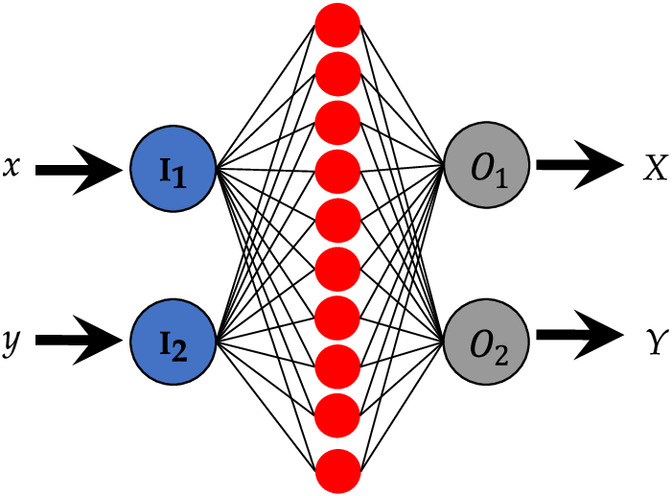
Typically, the unknown parameters are represented by weights and biases in a supervised feed-forward neural network. A feed-forward neural network is an artificial neural network wherein connections between the neurons do not form a cycle. In that case, the network is said to be fully connected in the sense that every node (also called neuron) in each layer of the network is connected to every node in the adjacent forward layer. For example, it can be formulated aswhere is the output vector with observations, is the activation function for the neuron in the output layer (green node), (green lines) are the unknown weights between the neuron in the output layer and each neuron in the hidden layer (blue nodes), is the activation function for each neuron in the hidden layer, (blue lines) are the unknown weights relative to the neurons in the hidden layer and each observation of the input data in the input-layer (red node), is the unknown bias for each neuron in hidden layer, and denotes the unknown bias for the output layer . Note that there is a weight for each observation of the input data. In other words, the larger the input sample, the more weights there are in that neural network. This is a simple case of considering only an input pattern and an output pattern. Obviously, the model in [Eq. (2)] can be extended to the case where we have more than one hidden layer and several inputs and outputs.
(2)
The activation functions in the hidden layer () are often either logistic-sigmoid (logsig) or hyperbolic tangent-sigmoid ()where is any input variable. In the case of [Eq. (2)], the is the result of the linear combination of the observations of the input data, weights, and bias (i.e., the second summation term). The output units usually have a purely linear transfer function of the type .
(3)
Usually, the back-propagation learning algorithm is employed in conjunction with a training algorithm to determine the weights and biases of a neural network. Since the transfer function involved in the neural networks is not linear [see Eq. (3)], a nonlinear least squares method that iteratively minimizes the mean squared errors between the desired outputs and the outputs response from the network is required (note: the index represents a given output attribute and an nth element of that attribute). In each epoch (iteration), therefore, the weights and biases are updated in a supervised manner by the following minimizationwhere represents the average squared error over the sample size for outputs.
(4)
Here, we use the Levenberg–Marquardt algorithm (LM), also known as the damped least squares method. The LM combines two minimization methods: the gradient-descent method (Newton-Raphson) and the Gauss-Newton method (Levenberg 1944). In the gradient-descent method, the mean squared errors () is reduced by updating the parameters in the steepest-descent direction. In the Gauss-Newton method, is reduced by assuming the least squares function is locally quadratic and finding the minimum of the quadratic form. The LM method acts more like a gradient-descent method when the parameters are far from their optimal value and acts more like the Gauss-Newton method when the parameters are close to their optimal value (Gavin 2020).
As mentioned, the available data are often split into three categories: training set, validation set, and test set. In the back-propagation algorithm, the first step in constructing a neural network is to adjust the weights and biases by using the training set. The performance of the model is often evaluated on the validation set at the end of each iteration (epoch). The aim of the validation set is to improve the generalization of the network learning. When the network starts to over-fit the training set, the performance on the validation set typically begins to decrease. When the validation error increases for a specified number of epochs the training is stopped, and the weights and biases at the minimum of the validation error are returned. This method for avoiding overfitting is called early stopping (Reitermanová 2010). Finally, the test set is used to evaluate the performance of the trained neural network, which theoretically guarantees an unbiased evaluation.
In practice, however, the test set does not guarantee an unbiased evaluation and prediction. If the data is a random sample, an estimate in [Eq. (1)] differs from the true value of because of the sampling error. Consequently, if this network is used to determine a prediction for some new input vector , the prediction will be different from the true prediction. Furthermore, as mentioned before, there is a randomness related to both the data splitting and randomness related to the network itself including architecture (number of hidden layers and the structure of the connections), weights and biases, initialization, and learning procedure. In this paper, resampling approaches are used to approximate a sampling distribution of the prediction and estimate parameters of that distribution like its mean value, variance, percentiles, etc.
Extension of Jackknife Resampling Methods for Prediction
Before starting, it is important to say that the cross-validation here is against the test set, not with respect to the validation set. The total training set is the set without the test set, in other words, it is the set including the training and validation data. Now, suppose that we divide the available dataset of size into groups of size , where . In that case, the equation [Eq. (1)] becomes
(5)
Then we can use one group to validate the performance of the training on the remaining () groups. The resulting estimator is said to be unbiased with respect to the test set. This process is repeated for all groups. For example, if and , one will get five groups of size . In machine learning language, this method is known as K-fold cross-validation. However, if the number of observations is a prime number and , the data cannot be divided into groups of the same size, since is not divisible by . Consequently, K-fold provides an unbalanced cross-validation, because one group will be larger than another. In addition, each point that was left out of the training set will be predicted only once.
To overcome this limitation, we can validate the subset of size and train the remaining observations at a time. This method is called Delete-d Jackknife. The subset size is chosen from all of the observations without replacement. In that case, instead of having only one single particular neural network predictor, we will have hundreds or even thousands predictors. This means that instead of making a single point prediction, we can describe its empirical distribution. In other words, this gives us the opportunity to do an interval prediction instead of just a one point prediction. Following this, the number of possible combinations for independent cross-validation, denoted by , and the number of repetitions of each point prediction () are given respectively by
(6)
(7)
For example, if and , one will get independent subset of cross-validations, with independent repetitions for each prediction point. Note that one will also get 171 neural networks predictors. This is the general case for Jackknife resampling. The extreme version of this strategy is to take , which is the same as taking in [Eq. (6)]. It means that each test set will contain one sample point. This is the idea of the Delete-1 Jackknife, in which each observation is validated with respect to the remaining () observations. Since the test set is chosen to be exactly of equal size, the Delete-1 Jackknife is also a balanced version of cross-validation. For example, in the case of having , we would have 19 trained neural networks with each point predicted once. Therefore, the main drawback of the Delete-1 Jackknife is that each output will be predicted only once, making it impossible to analyze the uncertainties.
Here, on the other hand, we take advantage of the idea of making several realizations (trials) of Delete-1 Jackknife to assess the probability distribution for the neural predictor rather than only the point predictor. In other words, the splitting data is fixed by taking , but with many trials (denoted by ). For example, if and the number of trials is , one will get neural network predictors, which provides 500 predictions for each single test point sample. This also allows us to capture the randomness related to the neural network itself including architecture, initialization, and the learning procedure. We termed this method Delete-1 Jackknife Trials. In this case, the number of neural network predictors will be equal to .
The accuracy of the Jackknife resampling methods depends on the choice of the number of the groups which will be deleted from the neural network training process (i.e, ). In general, the more observations in a training set, the better the network in terms of learning. However, the choice of still depends on the application. In the case of having independent and identically distributed variables (i.i.d.), the choice of the Delete-1 Jackknife Trials (i.e. or ) should give the most accurate assessment, since the training set is almost equal to . The problem is that independence is not always guaranteed. For instance, the independence assumption is invalid for time series data. Therefore, Delete-d Jackknife () would be more suitable in this case.
Actually, if the variables are not i.i.d. from the underlying distribution, then an even more suitable way of cross-validation is to use the idea of Hold-Out Trials. In that case, as previously mentioned, we randomly divide the total sample available in training and test and take several realizations () to obtain the interval prediction. Although we have fixed the number of subsets in each category (total training and test), their selection is made at random. For example, if and we randomly divide the sample into 85% total training and 15% test for , each point prediction will be repeated approximately 30 times. Therefore, the number of repetition of each point prediction is inexact, although it can be given approximately by Eq. (7). In the Hold-Out Trial, the number of neural network predictors is equal to the number of trials .
As previously mentioned, the most likely estimate (expected value) of an output quantity is not based only on one single prediction, but rather on an interval basis. For this, we sort the predicted values of a point into a strictly increasing order. The sorted predicted values provide an empirical distribution function for each output point (denoted by ). Then, for a stipulated coverage probability (denoted by ) we are be able to compute the desired percentiles as follows:where denotes rounding down to the next integer that indicates the position of the selected elements in the ascending order of . This position corresponds to a prediction for a stipulated overall probability . This can be done for any . This procedure is very similar to that found for the computation of critical values of outlier statistical tests (Lehmann 2012; Rofatto et al. 2020).
(8)
The resampling methods presented here also allow us to measure the prediction performance for the entire sample set. This is due to the fact that all sampling points participate in the test set. The root mean squared error (RMSE) on the test set was used to measure the accuracy of the prediction of each point as follows:where are the predicted values for each sample point and are the true output values. RMSE has been used as a standard statistical parameter to measure model performance in several applications. The RMSE indicates how far the output responses of the neural network are from the true outputs (targets) for each . Note that RMSE is computed for each of the available sample points. Although this expression represents the RMSEs for a single output, it can be computed to the case where one more output is available.
(9)
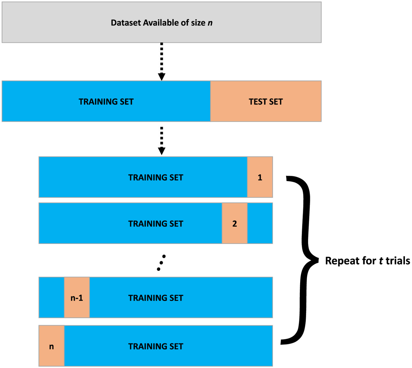
To make it clearer, the procedure associated with Delete-1 Jackknife Trials is summarized step-by-step as follows (Fig. 1):
1.
The dataset available of size is divided into two parts: training and test sets.
2.
Train the model with () observations and evaluate it using the remaining observation. For instance, given x as the input and y as the output variable in neural network, we would have as the training set, and the remaining observation () would be used to evaluate the model.
3.
Repeat the procedure in (2) times, excluding at each moment a different observation until all the observations have been deleted.
4.
The procedure in (2) and (3) is repeated a certain number of times (number of trials t). For example, if and the number of trials (denoted by t) is , one will get neural network predictors, which is 500 predictions for each single test point sample. In this case, the number of neural network predictors will be equal to .
Both Delete-d Jackknife and Hold-Out Trials are similar to Delete-1 Jackknife Trials. In the case of Delete-d Jackknife the training is performed with observations, without the need to define a number of trials, as explained previously by Eqs. (6) and (7). Finally, in the case of Hold-out, the dataset available is first randomly divided into training and testing, and it is repeated a certain number of times to quantify the uncertainties of the predictions.
Experiments and Results
Here we use resampling methods in neural networks and apply them to coordinate transformation. The coordinate transformation is a classic problem that always arises in various fields of engineering sciences, such as to convert coordinates from one geodetic reference system into another one (Ziggah et al. 2019a), to transform of 3-D point clouds from terrestrial laser scanning for deformation monitoring (Wujanz et al. 2018), to design and optimize geodetic networks (Teunissen 1985) and so on.
As a truly practical application, we present a problem of spatial transformation. In spatial transformation, each point of an input coordinate system is mapped to an output coordinate system. In this study, the input system corresponds to the image’s pixel indices (numCols, numRows), where numCols and numRows are the number of columns and rows in the image, respectively. We can specify locations in terms of their columns () and rows () and, therefore, it is a left-handed coordinate system. On the other hand, the output system is related to the grid body-fixed coordinate system, which in this case is a grid designed on white paper (Fig. 2).
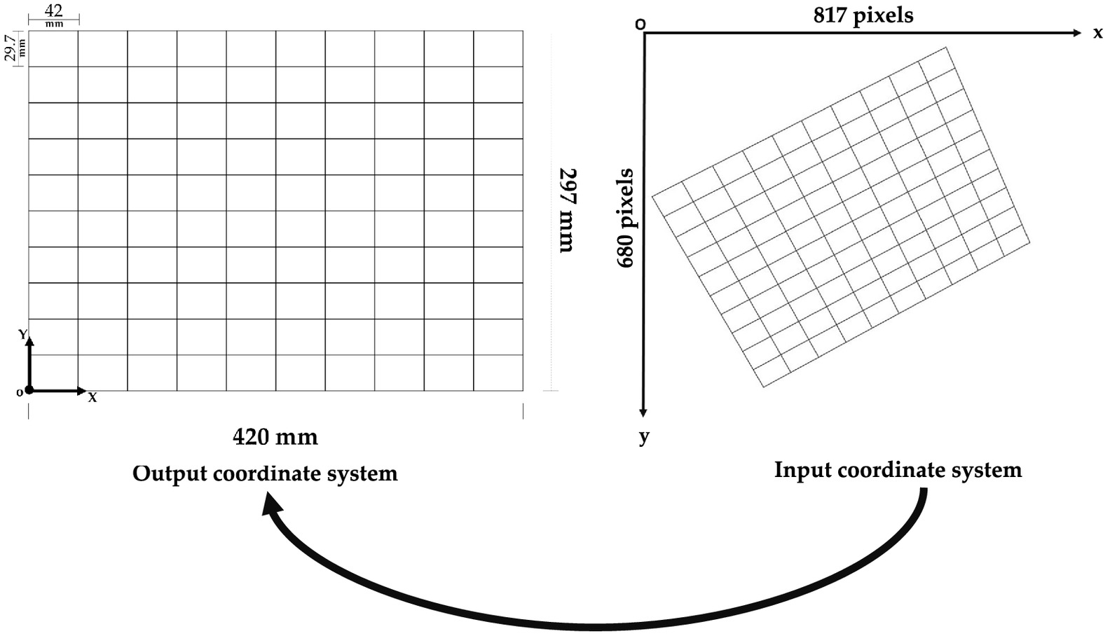
The origin of the output system is defined by the intersection of the first vertical line on the left and the first horizontal line at the bottom, which has coordinates. The horizontal and vertical axes are parallel to the grid width and height, respectively. It is therefore a right-handed coordinate system. The output system does not allow coordinates with negative values.
In general, we have the fixed coordinates in the output system and the observed coordinates in the input system , where denotes the point number. Since the grid dimension is and each point is offset by 42 mm in the X-direction and 29.7 mm in the Y-direction, we have a total of 121 points. All of these points were also selected in the image system. The image used here was captured by a cell phone camera at a distance of from the target (grid). The dimensions of this image are . The image was acquired with a camera oriented obliquely.
The choice related to the architecture, initialization, and learning procedure for the coordinate transformation problem was fixed here. The experiments were designed by considering one hidden layer composed of ten neurons (Fig. 3). The input data are the coordinates from the image system and the output data are the coordinates from the grid body-fixed coordinate system .
The training algorithm used here is the Levenberg–Marquardt back-propagation algorithm (LM). The Nguyen-Widrow algorithm was used to initialize the weights and biases (Nguyen and Widrow 1990). Levenberg’s contribution provided a “damped version” of the minimization problem for [Eq. (4)] (Gavin 2020)where is the Jacobian matrix containing first derivatives of with respect to the weights and biases; is the identity matrix, providing increment to the weights and biases estimated parameters . Note that are the desired outputs and are the output’s response from the network.
(10)
The non-negative damping factor () in Eq. (10) is adjusted at each iteration. If the reduction of the mean squared errors in equation Eq. (4) is quick, a smaller value can be used, bringing the algorithm closer to the Gauss-Newton algorithm, but if an iteration gives insufficient reductions to the error, can be increased, which would provide a step closer to the gradient-descent direction. Note that the gradient of with respect to is . This means that for large values of damping factor , the step will be taken approximately in the direction opposite to the gradient. In other words, if any iteration occurs to result in a worse approximation, i.e., , then is increased. On the other hand, as the solution improves, is decreased and the solution tends to go to the local minimum and, therefore, LM approaches the Gauss-Newton method (Madsen et al. 2004; Marquardt 1963; Gavin 2020).
The initial value of the damping factor adopted here was , with a decrease factor of 0.1 and increase factor of 10. The performance of the model was evaluated on the validation set at the end of each iteration (epoch). The aim of the validation set was to improve the generalization of the LM. When the network starts to over-fit the data, the performance on the validation set typically begins to decrease. When the validation error increases for a specified number of epochs the training is stopped, and the weights and biases at the minimum of the validation error are returned. This method for avoiding overfitting is called early stopping. The performance function is also given by the mean squared error in Eq. (4). We used the command-line functionality of the Matlab’s Neural Network toolbox (R2019b) for training and validating the neural network. Thus, the learning process was configured to stop when any of these conditions were met:
•
A maximum number of epochs (iteration) of 1,000 is reached.
•
The minimum performance gradient falls below .
•
.
•
The network performance on the validation set fails to improve or remains the same for six epochs.
The inputs and outputs values were normalized according to the z-score as follows:where represents the sample of the input or output of the neural network, is the mean of the sample, and is the standard deviation of the sample. In this case, the normalized function gives values between .
(11)
Resampling Methods in a Neural Network Applied to Coordinate Transformation
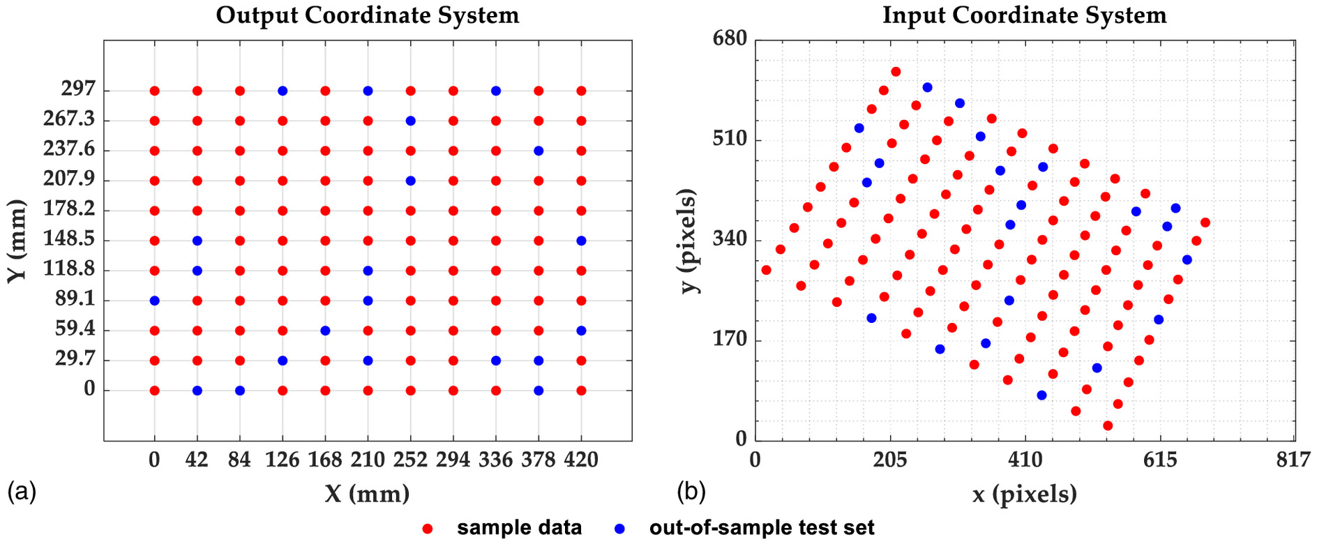
At first, we randomly selected 100 points from both coordinate systems for the application of resampling methods in the neural network. The remaining 21 points have not participated in any training, validation, or test procedures of the network. They were considered as out-of-sample sets to test resampling methods in neural network predictions (Fig. 4).
The subset size was chosen from all of the observations without replacement for the case of Delete-d Jackknife. Therefore, we got independent cross-validations and neural-network-based predictors from Eq. (6). In effect, we got repetitions for each point prediction from equation Eq. (7). For comparison, each resampling method was set up to have the same number of repetitions for each prediction point. Thus, Delete-1 Jackknife Trials was set up to have trials, which provides 99 repetitions for each point prediction and neural-network-based predictors and is twice as many predictors compared to Delete-d Jackknife with . In the case of Hold-Out Trials, we had to randomly divide the data into 88% (88 points) training set, 10% (10 points) validation set, and 2% (2 points) test set with trials . This gave us approximately repetitions for each point prediction and the same number of neural-network-based predictors of 4,950 as Delete-d Jackknife for . The training set was fixed with 88 points for all resampling methods.
The RMSE was computed according to Eq. (9), but now extended to two output neural network responses as follows:where and are the predicted values of and coordinates for each point of the grid, respectively; and and are the true and coordinates of each point of the grid (targets).
(12)
The bias of both coordinates and for each point were also computed by taking the difference between the most likely predicted value and the true value. In that case, the most likely values were computed by taking in the equation [Eq. (8)], which corresponds to the 50th percentile (i.e., the median) of the total number of predictions for each coordinate point . Thus, the resulting bias (denoted by ) was obtained through the Pythagorean decomposition between the bias in the X- and Y-directions as follows:where and represent the predictor bias for and of each grid point, respectively; and correspond to the 50th-percentile of the and coordinates for each point; and and are the true values of the grid coordinates.
(13)
(14)
(15)
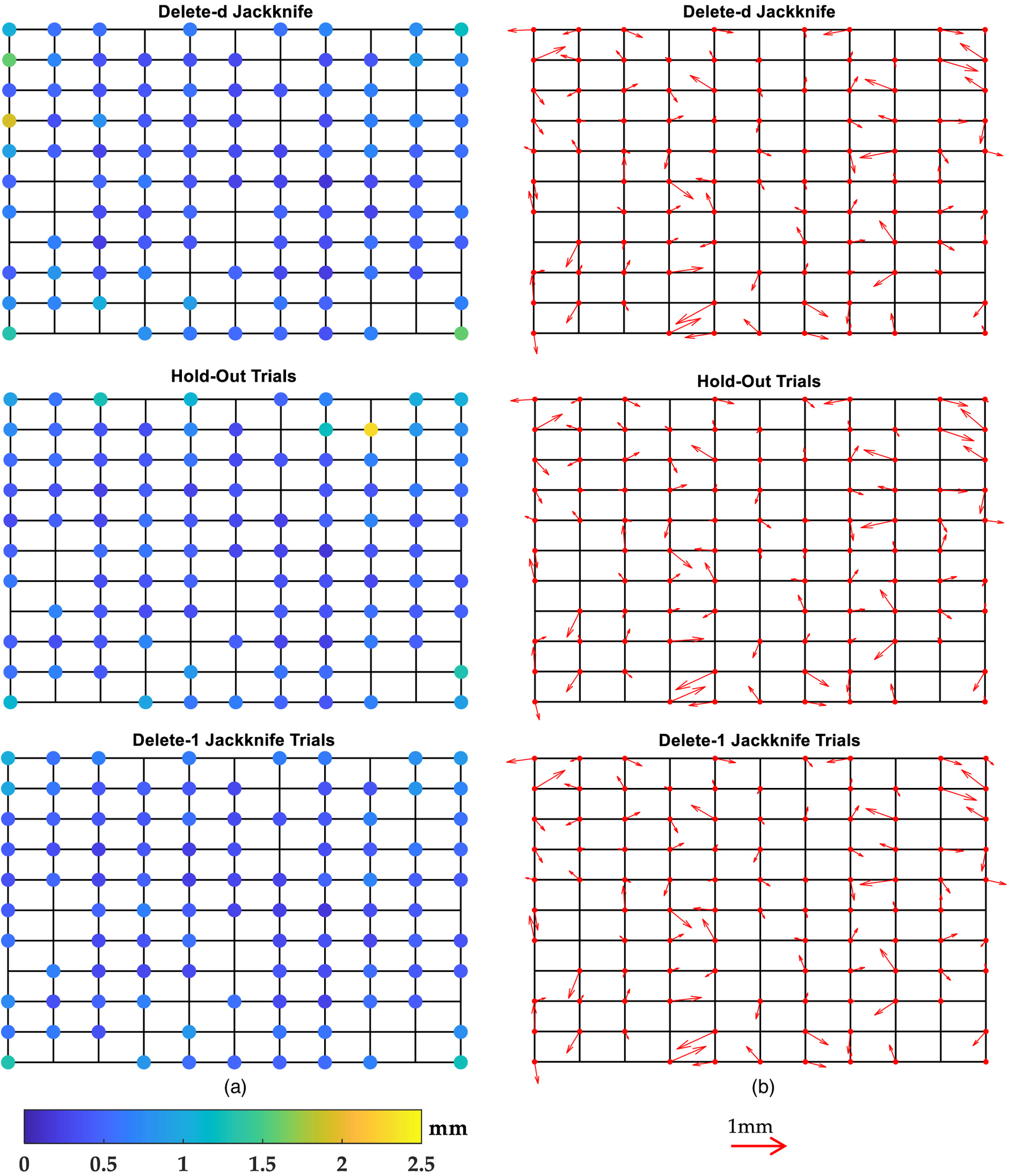
For this experiment, we had replicas of each point for both Jackknife methods and for Hold-Out Trials, with each RMSE and the resulting bias computed for each of the points. The RMSE and the resulting bias for each resampling method are displayed in Fig. 5. Table 1 summarizes the results of the resampling methods, listing the deletes of the data for test set (), number of trials (), number of all possible combinations (), number of repetitions of each point prediction (Repetitions), number of neural-network-based predictors, and the overall statistics of the RMSEs (mean, standard deviation, maximum and minimum) for each case.
| Resampling method | Repetitions | Number of predictors | Average RMSE | Max. RMSE | Min. RMSE | |||
|---|---|---|---|---|---|---|---|---|
| Jack-d | 2 | — | 4,950 | 99 | 4,950 | 0.56 () | 1.92 | 0.17 |
| Jack-1 | 1 | 99 | 100 | 99 | 9,900 | 0.50 () | 1.31 | 0.18 |
| H-out | 2 | 4,950 | — | 4,950 | 0.55 () | 2.28 | 0.17 |
Analysis of the Resampling Methods on the Out-of-Sample Test Set
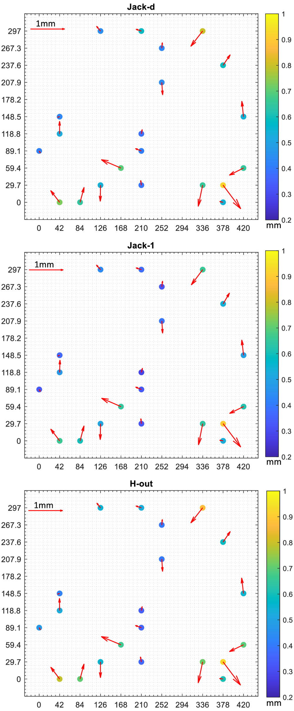
In this section, we evaluated the performance of the resampling methods based on the out-of-sample test set, which means that no decision was made using this test set during the resampling process. As mentioned previously, this set corresponds to 21 points points that have not participated in training, validation, or the test set. This may provide an unbiased evaluation. The number of neural network-based predictors applied to each of the 21 points was larger for Delete-1 Jackknife Trials (Jack-1: 9,900) than both Delete-d Jackknife (Jack-d: 4,950) and Hold-Out Trials (H-out: 4,950), as can be seen in Table 1. Fig. 6 displays the results of applying the neural-networks-based predictors constructed from Delete-d Jackknife (Jack-d), Delete-1 Jackknife Trials (Jack-1), and Hold-Out Trials (H-out), respectively. Table 2 summarizes the results of the application of the neural-network-based predictors on the out-sample-test set.
| Resampling method | Average RMSE | Max. RMSE | Min. RMSE | Average bias | Max. bias | Min. bias |
|---|---|---|---|---|---|---|
| Jack-d | 0.56 () | 0.92 | 0.38 | 0.31 () | 0.78 | 0.05 |
| Jack-1 | 0.50 () | 0.90 | 0.28 | 0.30 () | 0.77 | 0.05 |
| H-out | 0.57 () | 0.92 | 0.35 | 0.30 () | 0.77 | 0.06 |
Discussion
From Fig. 5, we observe that both the magnitude and the direction of the biases occurred in different ways at each point. In other words, the biases had a random behavior. The biases were less than 1 mm for all resampling methods. Considering all points, the biases averaged 0.31 mm () for all resampling methods. In terms of the evaluation of the resampling methods on the out-of-sample test set, Jack-1 was also slightly better than the other two methods, as seen in Table 2. From Fig. 6, again, the biases had a random behavior, and in that case, both biases and the RMSE exhibited values less than 1 mm.
Table 1 and Fig. 5 show that, in terms of RMSE, Jack-1 is slightly better [0.50 mm ()] than Jack-d [0.56 mm ()] and H-out [0.55 mm ()]. This is also true for the results of the application of neural-network-based predictors derived from the resampling methods on the out-of-sample test set in Table 2. This can be explained by the fact that the training set is almost equal to the number of observations . In other words, choosing in Eq. (6) should give the most accurate assessment. To support this analysis, we also apply resampling methods with different configurations and their results are displayed in Table 3.
| Resampling method | Repetitions | Number of predictors | Average RMSE | Max. RMSE | Min. RMSE | |||
|---|---|---|---|---|---|---|---|---|
| H-out | 1 | 9,900 | — | 9,900 | 0.53 () | 1.89 | 0.17 | |
| Jack-1 | 1 | 1,000 | 100 | 1,000 | 100,000 | 0.65 () | 12.45 | 0.22 |
| H-out | 1 | 100,000 | — | 100,000 | 0.64 () | 8.26 | 0.21 | |
| Jack-d | 3 | — | 161,700 | 4,851 | 161,700 | 0.73 () | 5.52 | 0.27 |
| H-out | 3 | 161,700 | — | 161,700 | 0.89 () | 20.67 | 0.25 |
Table 3 shows that the H-out method for and trials of provides similar results of Jack-1 for in Table 1. It is important to note that there are no advantages to increasing both the number of trials and the number of the validation subsets . Note that the RMSE worsened when increasing even to . This is due to the fact that there are more chances of overfitting or underfitting when increasing the trials . Consequently, in using the resampling process, there are certain chances that one or more predictions will deviate significantly from their true value, as can be seen by the maximum RMSE in Table 3.
Conclusions
Resampling methods can be used with powerful computers to construct inferential procedures in modern statistical data analysis. They replace theoretical derivations required in applying traditional methods by repeatedly resampling the original data and making inferences from the re-samples. In this contribution, we introduce three resampling methods in neural networks, namely Delete-d Jackknife (Jack-d), Delete-1 Jackknife Trials (Jack-1), and Hold-Out Trials (H-out).
The Jack-d method consists of separating the dataset into a subset of size and training the remaining each of the observations one at a time. The subset size d is selected from all of the observations without replacement. The Jack-1 method is an extension of the classical Delete-1 Jackknife by taking and training each of the remaining observations one at a time and by drawing many realizations (trials). Similar to Jack-1, Hold-out is also extended to its H-out version by randomly drawing many realizations, so that each prediction point is repeated a certain number of times. The user knows exactly the number of times each point prediction will be replicated for the cases where Jack-d and Jack-1 are in play. On the other hand, in the case of the H-out method, the user chooses the percentage of division of the sample for each set (training, validation and test) and the number of realizations (trials). An advantage of these resampling techniques is that they allow us to determine the approximate probability distribution for the predictor rather than simply providing a point prediction. A consequence of this is that in addition to all points passing through the test set, they are often tested using different training processes. By nature, neural networks are non-deterministic due to random initialization of the weights, biases, and different optimization techniques. Therefore, the training of a neural network is different for each trial due to this randomness associated with the neural network.
A neural-network-based on resampling methods was applied to a problem of coordinate transformations. The results suggest that, in general, the accuracy of the resampling methods is based on the choice of the size of the test set and the number of realizations (trials). The smaller the test group, the better the accuracy of the neural network model, since the training set is almost equal to the dimension of the dataset. There are no advantages to increasing both the number of trials and the number of the test subsets . Wang and Yu (2020) showed that the optimal is obtained by approaching its value to for the case of parameter estimation by the weighted total least squares. In terms of a neural network for prediction, however, our results show that the optimal choice is driven in favor of a smaller . However, in higher dimensional problems, both Jack-1 and Jack-d can lead to an increase in computational time for neural network learning. In that case, H-out with a larger test set should be more appropriate. Here, we are concerned less about the best selection of the neural network parameters. Instead, our key point is with respect to describing the quality of the neural network predictor. In future works, we will address efforts in the application of resampling methods to find the best network parameters.
Furthermore, due to the randomness associated with the neural network, there are certain chances that one or more predictions by the resampling process will significantly deviate from their true value. These deviations are understood to be outliers. Specifically, the Levenberg–Marquardt method used here is very sensitive to the initial network weighs. In addition, it does not consider outliers in the data. In fact, some realizations may have been overfitted. Since we have several predictions for each variable of output of the neural network, it is possible to remove those outliers. Therefore, outlier filtering methods will be studied and discussed in future works.
In the case of having independent and identically distributed variables (IIDs), the choice of Jack-1 should give the most accurate evaluation, since the training set is almost equal to the size of the dataset. The problem is that independence is not always guaranteed. For instance, the independence assumption is invalid for time series data. Therefore, Jack-d would be more suitable in this case. Actually, if the variables are not IIDs with respect to the underlying distribution, then an even more suitable way of resampling is to use the idea of H-out. In future studies, this issue will be addressed in detail.
Data Availability Statement
Some or all data, models, or code generated used during the study are available in a repository online in accordance with funder data retention policies (Rofatto and Matsuoka 2022).
References
Burman, P. 1989. “A comparative study of ordinary cross-validation, v-fold cross-validation and the repeated learning-testing methods.” Biometrika 76 (3): 503–514. https://doi.org/10.1093/biomet/76.3.503.
Efron, B. 1980. The Jackknife, the bootstrap, and other resampling plans. Stanford, CA: Stanford Univ.
Efron, B. 1982. “The Jackknife, the bootstrap and other resampling plans.” Accessed November 4, 2021. https://epubs.siam.org/doi/abs/10.1137/1.9781611970319.
Efron, B. 1992. “Jackknife-after-bootstrap standard errors and influence functions.” J. R. Stat. Soc. Ser. B 54 (1): 83–127.
Farolfi, G., and C. Del Ventisette. 2016. “Contemporary crustal velocity field in alpine Mediterranean area of Italy from new geodetic data.” GPS Solut. 20 (4): 715–722. https://doi.org/10.1007/s10291-015-0481-1.
Gavin, H. P. 2020. The Levenberg-Marquardt algorithm for nonlinear least squares curve-fitting problems. Durham, NC: Duke Univ.
Haykin, S. 1999. Neural networks a comprehensive foundation. 2nd ed. Englewood Cliff, NJ: Prentice Hall.
Kaloop, M. R., and D. Kim. 2014. “Gps-structural health monitoring of a long span bridge using neural network adaptive filter.” Survey Rev. 46 (334): 7–14. https://doi.org/10.1179/1752270613Y.0000000053.
Kavzoglu, T., and M. H. Saka. 2005. “Modelling local gps/levelling geoid undulations using artificial neural networks.” J. Geod. 78 (9): 520–527. https://doi.org/10.1007/s00190-004-0420-3.
Lehmann, R. 2012. “Improved critical values for extreme normalized and studentized residuals in Gauss–Markov models.” J. Geod. 86 (12): 1137–1146. https://doi.org/10.1007/s00190-012-0569-0.
Levenberg, K. 1944. “A method for the solution of certain non-linear problems in least squares.” Q. Appl. Math. 2 (2): 164–168. https://doi.org/10.1090/qam/10666.
Lin, L.-S. 2007. “Application of a back-propagation artificial neural network to regional grid-based geoid model generation using gps and leveling data.” J. Surv. Eng. 133 (2): 81–89. https://doi.org/10.1061/(ASCE)0733-9453(2007)133:2(81).
Liu, X., J. Liang, Z.-Y. Wang, Y.-T. Tsai, C.-C. Lin, and C.-C. Chen. 2020. “Content-based image copy detection using convolutional neural network.” Electronics 9 (12): 2029. https://doi.org/10.3390/electronics9122029.
Madsen, K., N. B. Nielsen, and O. Tinglef. 2004. Methods for nonlinear least squares problems. Lyngby, Denmark: Technical Univ. of Denmark.
Marquardt, D. W. 1963. “An algorithm for least-squares estimation of nonlinear parameters.” J. Soc. Ind. Appl. Math. 11 (2): 431–441. https://doi.org/10.1137/0111030.
McIntosh, A. 2016. “The Jackknife estimation method.” Preprint, submitted June 1, 2016. http://arxiv.org/abs,arXiv:1606.00497.
Miller, R. G. 1974. “The Jackknife—A review.” Biometrika 61 (1): 1–15. https://doi.org/10.2307/2334280.
Mollalo, A., L. Mao, P. Rashidi, and G. E. Glass. 2019. “A gis-based artificial neural network model for spatial distribution of tuberculosis across the continental united states.” Int. J. Environ. Res. Public Health 16 (1): 157. https://doi.org/10.3390/ijerph16010157.
Nguyen, D., and B. Widrow. 1990. “Improving the learning speed of 2-layer neural networks by choosing initial values of the adaptive weights.” In Vol. 3 of Proc., IJCNN Int. Joint Conf. on Neural Networks, 21–26. New York: IEEE.
Pan, L. 1998. “Resampling in neural networks with application to financial time series.” Ph.D. thesis, Faculty of Graduate Studies, Univ. of Guelph.
Quenouille, M. H. 1949. “Approximate tests of correlation in time-series.” J. R. Stat. Soc. Ser. B 11 (1): 68–84.
Reitermanová, Z. 2010. “Data splitting.” In Proc., Contributed Papers, Part I: Mathematics and Computer Sciences, edited by J. Šafránková and J. Pavlȯu. Prague, Czech Republic: MATFYZPRESS.
Rofatto, V., and M. Matsuoka. 2022. “Resampling for coordinate transformation.” Mendeley Data V1. Accessed February 24, 2022. https://doi.org/10.17632/cddjxjyrh4.1.
Rofatto, V. F., M. T. Matsuoka, I. Klein, M. Roberto Veronez, and L. G. da Silveira. 2020. “A Monte Carlo-based outlier diagnosis method for sensitivity analysis.” Remote Sens. 12 (5): 860. https://doi.org/10.3390/rs12050860.
Sothe, C., et al. 2020. “Evaluating a convolutional neural network for feature extraction and tree species classification using uav-hyperspectral images.” ISPRS Ann. Photogramm. Remote Sens. Spatial Inf. Sci. V-3-2020: 193–199. https://doi.org/10.5194/isprs-annals-V-3-2020-193-2020.
Stopar, B., T. Ambroi, M. Kuhar, and G. Turk. 2006. “Gps-derived geoid using artificial neural network and least squares collocation.” Surv. Rev. 38 (300): 513–524. https://doi.org/10.1179/sre.2006.38.300.513.
Teunissen, P. 1985. “Zero order design: Generalized inverses, adjustment, the datum problem and s-transformations.” In Optimization and design of geodetic networks, edited by E. W. Grafarend and F. Sansò, 11–55. Berlin: Springer.
Tierra, A., R. Dalazoana, and S. D. Freitas. 2008. “Using an artificial neural network to improve the transformation of coordinates between classical geodetic reference frames.” Comput. Geosci. 34 (3): 181–189. https://doi.org/10.1016/j.cageo.2007.03.011.
Tukey, J. W. 1958. “Bias and confidence in not-quite large samples.” Ann. Math. Stat. 29 (2): 614–623. https://doi.org/10.1214/aoms/1177706647.
Wang, L., Z. Li, and F. Yu. 2022. “Jackknife method for the location of gross errors in weighted total least squares.” Commun. Stat. Simul. Comput. 51 (4): 1946–1966. https://doi.org/10.1080/03610918.2019.1691225.
Wang, L., and F. Yu. 2020. “Jackknife resampling parameter estimation method for weighted total least squares.” Commun. Stat. Theory Methods 49 (23): 5810–5828. https://doi.org/10.1080/03610926.2019.1622725.
Wang, L., and F. Yu. 2021. “Jackknife resample method for precision estimation of weighted total least squares.” Commun. Stat. Simul. Comput. 50 (5): 1272–1289. https://doi.org/10.1080/03610918.2019.1580727.
Wang, L., F. Yu, Z. Li, and C. Zou. 2020. “Jackknife method for variance components estimation of partial eiv model.” J. Surv. Eng. 146 (4): 04020016. https://doi.org/10.1061/(ASCE)SU.1943-5428.0000327.
Wood, M. 2005. “Bootstrapped confidence intervals as an approach to statistical inference.” Organizational Res. Methods 8 (4): 454–470. https://doi.org/10.1177/1094428105280059.
Wujanz, D., M. Avian, D. Krueger, and F. Neitzel. 2018. “Identification of stable areas in unreferenced laser scans for automated geomorphometric monitoring.” Earth Surf. Dyn. 6 (2): 303–317. https://doi.org/10.5194/esurf-6-303-2018.
Yang, F., J. Guo, C. Zhang, Y. Li, and J. Li. 2021a. “A regional zenith tropospheric delay (ZTD) model based on GPT3 and ANN.” Remote Sens. 13 (5): 838. https://doi.org/10.3390/rs13050838.
Yang, G., K. C. P. Wang, J. Q. Li, Y. Fei, Y. Liu, K. C. Mahboub, and A. A. Zhang. 2021b. “Automatic pavement type recognition for image-based pavement condition survey using convolutional neural network.” J. Comput. Civ. Eng. 35 (1): 04020060. https://doi.org/10.1061/(ASCE)CP.1943-5487.0000944.
Ziggah, Y. Y., Y. Hu, Y. Issaka, and P. B. Laari. 2019a. “Least squares support vector machine model for coordinate transformation.” Geod. Cartography 45 (5): 16–27. https://doi.org/10.3846/gac.2019.6053.
Ziggah, Y. Y., H. Youjian, A. Tierra, A. A. Konaté, and Z. Hui. 2016. “Performance evaluation of artificial neural networks for planimetric coordinate transformation—A case study, ghana.” Arabian J. Geosci. 9 (17): 698. https://doi.org/10.1007/s12517-016-2729-7.
Ziggah, Y. Y., H. Youjian, A. R. Tierra, and P. B. Laari. 2019b. “Coordinate transformation between global and local datums based on artificial neural network with k-fold cross-validation: A case study, Ghana.” Earth Sci. Res. J. 23 (1): 67–77. https://doi.org/10.15446/esrj.v23n1.63860.
Information & Authors
Information
Published In

Journal of Surveying Engineering
Volume 149 • Issue 1 • February 2023
Copyright
This work is made available under the terms of the Creative Commons Attribution 4.0 International license, https://creativecommons.org/licenses/by/4.0/.
History
Received: Feb 25, 2022
Accepted: Sep 2, 2022
Published online: Dec 9, 2022
Published in print: Feb 1, 2023
Discussion open until: May 9, 2023
Authors
Metrics & Citations
Metrics
Citations
Download citation
If you have the appropriate software installed, you can download article citation data to the citation manager of your choice. Simply select your manager software from the list below and click Download.