Design and Control Benchmark of Rib-Stiffened Concrete Slabs Equipped with an Adaptive Tensioning System

Reksowardojo, Arka P.; Senatore, Gennaro; Bischoff, Manfred; Blandini, Lucio

doi:10.1061/JSENDH.STENG-12320

Open access

Technical Papers

Oct 28, 2023

Design and Control Benchmark of Rib-Stiffened Concrete Slabs Equipped with an Adaptive Tensioning System

Authors: Arka P. Reksowardojo, Ph.D., A.M.ASCE https://orcid.org/0000-0002-5626-430X, Gennaro Senatore, Ph.D. https://orcid.org/0000-0001-7418-9713 [email protected], Manfred Bischoff, Dr.Ing. https://orcid.org/0000-0003-1538-4281, and Lucio Blandini, Dr.Ing. https://orcid.org/0000-0002-4592-6347Author Affiliations

Publication: Journal of Structural Engineering

Volume 150, Issue 1

https://doi.org/10.1061/JSENDH.STENG-12320

PDF

Abstract

Floor systems are typically designed to satisfy tight deflection limits under out-of-plane loading. Although the use of concrete flat slabs is common in the built environment due to the ease of construction, the load-bearing performance is inefficient because the material is not optimally distributed within the cross section to take the bending caused by external loads. This typically results in significant oversizing. Floor slabs account for more than 50% of the material mass and associated emissions embodied in typical low-rise reinforced concrete buildings. In addition, the volume of carbon-intensive cement production has tripled in the last three decades. Therefore, lightweight floor systems that use minimum material resources causing low emissions can have a significant impact on reducing adverse environmental impacts of new constructions. Recent work has shown that rib-stiffened slabs offer significant potential for material savings compared with flat slabs. This work investigates adaptive rib-stiffened slabs equipped with an adaptive tensioning system. The adaptive tensioning system comprises cables embedded within the concrete rib through a duct that enables varying the cable tension as required to counteract the effect of different loading conditions without applying permanent prestress that might cause unwanted long-term effects including tension loss and amplified deflection. The cables are positioned following a profile so that the tension force is applied eccentrically to the neutral axis of the slab-ribs assembly. The resulting system of forces causes a bending moment that counteracts the effect of the external load. The rib placement is optimized through a greedy algorithm with a heuristic based on the direction of the principal stresses. The deflection of the slab is reduced by adjusting the cable tensile forces computed by a quasi-static controller. Benchmark studies comparing different cable profiles and active rib layouts are carried out to determine an efficient control configuration. A case study of an

8 \times 8 - m

adaptive rib-stiffened slab is implemented to evaluate material savings potential. Results show that the adaptive slab solution can achieve up to 67% of material savings compared with an equivalent passive flat slab.

Introduction

Previous Work

Civil structures are designed to satisfy strength and deformation criteria under strong and rarely occurring loads. Consequently, the structural capacity is underutilized for most of the service life. However, the building sector is globally responsible for 40% of the energy use (European Commission 2016) and 50% of the material consumption (OECD 2019). The volume of carbon-intensive cement production tripled between 1995 and 2014 and has since continued growing to fulfill demands in emerging countries (USGS 2016; Olivier et al. 2017; Andrew 2019). It has therefore become important to minimize the environmental impact of load-bearing structures made with concrete.

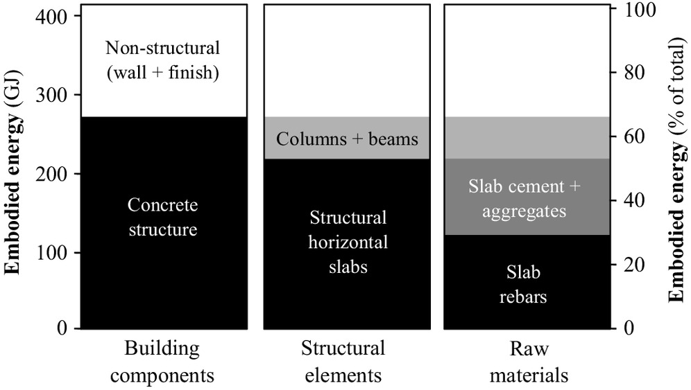
Construction projects generally involve large amounts of embodied energy and emissions, associated with the extraction, manufacturing, and transport of material as well as the fabrication and assembly of structural and architectural components. As illustrated in Fig. 1, floor slabs account for more than 50% of the total energy embodied in typical low-rise reinforced concrete buildings (Berger et al. 2013; Huberman et al. 2015). The ease of construction has greatly contributed to the widespread use of constant-thickness flat slabs. However, the load-bearing performance of flat slabs is generally inefficient because the material is distributed uniformly within the cross section while the load is transferred through bending. Typical design practice involves satisfying relatively tight deflection limits (e.g., span/500) under strong loads, which results in flat slabs with a conservative 250–300-mm depth for spans up to 9 m.

Fig. 1. Breakdown of embodied energy in typical low-rise reinforced concrete frame construction. (Reprinted from *Energy and Buildings*, Vol. 104, N. Huberman, D. Pearlmutter, E. Gal, and I. A. Meir, “Optimizing structural roof form for life-cycle energy efficiency,” pp. 336–349, © 2015, with permission from Elsevier.)

Adaptive structures that can react to loading through sensing and actuation offer a potential solution to significantly reduce the material and energy impacts of load-bearing structures (Senatore et al. 2019; Senatore and Reksowardojo 2020; Blandini et al. 2022). Adaptive structures embody sensors and actuators to maintain an optimal structural state against changing load conditions through active control (Soong 1988). An extensive body of work exists on the actuation of discrete systems such as trusses and frames (Reinhorn et al. 1993; Senatore et al. 2011, 2018; Weidner et al. 2018; Reksowardojo et al. 2022). However, the actuation of continuous systems such as plates and shells has received little attention. Neuhäuser (2014) employed actuation through actively controlled supports h to modify the in-plane membrane stress state in a doubly curved timber shell structure when disturbances such as local loadings, fabrication imperfections, or residual stress formed after formwork removal occur.

A new actuation strategy has been developed for concrete beams through integrated fluidic actuators (Kelleter et al. 2020). The actuation system comprises a series of lens-shaped pressure chambers made of two welded steel sheets that are embedded into the beam cross section. For simply supported beams, the pressure chambers are placed in the upper region above the neutral axis. The chambers expand through hydraulic pressure thus generating compressive forces eccentric to the neutral axis. The resulting active bending moment is employed to counteract the effect of the external load, which reduces stress and deflections. Control of deformation and stress for two-way slabs using new types of fluidic actuators is under investigation (Nitzlader et al. 2022a, b). Actuation modes have been implemented according to the principal moments caused by external loads and target displacement reduction showing good potential for significant reduction of deformations and material savings.

When considering all costs involved including construction, solid slabs are often preferred because they are still perceived as optimal, especially for short and medium spans. However, considering the effort to reduce the adverse effects of climate change, ongoing material scarcity, and the advent of robotic fabrication, it is very likely that in the not-so-distant future, the cost of construction will become a fraction of the cost of material and embodied carbon, especially if policies to tax embodied carbon will be implemented. In this scenario, solid slabs will no longer be competitive solutions.

The improvement of load-bearing properties in plates and thin shells through the addition of monolithically-integrated stiffening beams, which are hereafter referred to as ribs, is a well-established strategy in various fields of engineering. Within the context of civil structures, linear- or crossed-grid configurations are often employed for rib-stiffened floor slabs. In the work of Nervi (1956), floor slabs were stiffened by curvilinear ribs placed following the principal stress directions (Nervi 1956; Iori 2012; Halpern et al. 2013). In this case, the principal stress directions were obtained through a photoelastic experiment on an equivalent flat slab; hence, the design process could not be generalized. Digital fabrication techniques might facilitate the wider adoption of slabs stiffened by an optimized rib layout, which has been limited due to fabrication challenges (Rippmann et al. 2018). Recent work has shown that the additional stiffness provided by an optimized rib layout allows for up to 50% material savings compared with equivalent flat slabs (Wu et al. 2020; Ranaudo et al. 2021).

Previous work on variable post-tensioning systems has shown that they are an effective solution to counteract deflection in concrete beams (Pacheco and Adao da Fonseca 2002; Schnellenbach-Held et al. 2013). An experimental study (Schnellenbach-Held and Steiner 2014) has shown that a significant reduction of tensile stress can be achieved using variable post-tensioning, which is desirable because the tensile capacity of concrete is poor. However, most previous implementations rely on model-free controllers, and thus the relationship between cable tension and the responses of the concrete beams has not been formulated explicitly.

New Contribution

This work offers a new methodology to design adaptive rib-stiffened concrete slabs. The aim is to provide a solution for early-stage design, which can be further elaborated through appropriate detailing. An adaptive tensioning system is employed, which comprises a steel cable embedded within the concrete rib through a duct that enables varying the cable tension as required. The cables are positioned following a profile so that the resulting system of forces causes a bending moment that counteracts the effect of the external load. Although this actuation strategy shares similarities with conventional prestressing, there are several important differences. The application of tensile forces in conventional prestressing is a one-time action, and thus it is only effective under a single load case. Instead, in this work a variable post-tensioning system is employed to counteract effectively different loading conditions without applying sustained prestressing that might cause unwanted permanent stress and might accelerate the onset of long-term effects including tension loss and amplified deflection.

Although similar variable tensioning systems have been investigated in previous work (Pacheco and Adao da Fonseca 2002; Schnellenbach-Held et al. 2013), no explicit formulation has been provided to compute the required tension forces to control the structural response. In this paper, an explicit relationship between cable tensions and the structural response is formulated. Based on this relationship, the slab deflection is reduced by adjusting the cable tension. The control commands are computed through a quasi-static controller that employs bounded least-square optimization. The proposed adaptive rib-stiffened slab system offers two advantages: (1) the geometry of the ribs allows actuation forces to be applied eccentrically to the neutral axis of the slab-ribs assembly, and (2) the concrete cover protects the actuation system from environmental agents. In the event of a strong loading event, deflections are actively controlled to satisfy serviceability limits. The ability to actively counteract the effect of loading generally results in significant savings of material and thus embodied energy and associated emissions.

In addition, no method has been previously formulated to include in a design process the effect of response control through similar adaptive tensioning systems. This work provides a new integrated structure-control optimization process that can be applied to two-way slabs, thus extending previous use cases that have focused mostly on beam components.

Active Rib

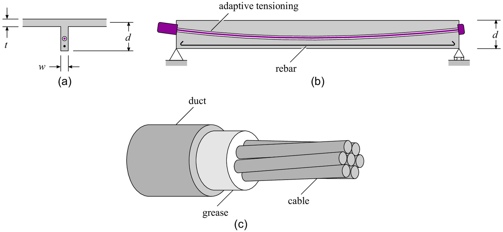
Figs. 2(a and b) illustrate an example of an active rib comprising a cable and a rebar placed in the lower region. For illustration, a cable with a parabolic profile is considered here. The slab thickness is denoted as

t

, and the width and the depth of the ribs are denoted

w

and

d

, respectively. The variable post-tensioning system consists of a steel cable, which is placed unbonded inside a grease-filled duct [Fig. 2(c)], and an actuator [Fig. 2(b)] that applies the required tension force by pulling on the cable. It is assumed that electromechanical actuators are used. The term unbonded refers to the absence of bonding between the duct and the cable. The inner diameter of the duct is larger than the external diameter of the cable to minimize mechanical contact. This allows the cable to slide with minimal resistance caused by friction with the duct and the grease viscosity.

Fig. 2. (a) Dimensions of an active rib; (b) longitudinal section of an active rib; and (c) detail of the adaptive tensioning system.

Design Method

The design process formulated in this work comprises two stages: (1) rib layout optimization, and (2) sizing optimization. The rib layout optimization is carried out first followed by sizing optimization of the slab and ribs. Both stages are formulated as optimization problems to minimize the material volume

V \in R

. The problem stated in Eqs. (1) and (2) is a formulation that is adopted in both stages, which differ primarily in the design variables.

In the rib layout optimization process, the variable vector

x

is a subset of an integer solution domain

Ω^{r} \in Z

. Each integer in

Ω^{r}

corresponds to a particular curve (i.e., a rib profile) in a predetermined layout (i.e., a set of curves). As a heuristic to aid the optimization process, the solution domain

Ω^{r}

is based on the direction of principal stresses for a flat slab with identical dimensions and boundary conditions under a uniformly distributed load. In the sizing optimization process, the solution vector

x \in R^{3}

comprises the thickness of the slab

t \in R

, the width of the ribs

w \in R

, and the depth of the ribs

d \in R

; therefore,

x = {[\begin{matrix} t & w & d \end{matrix}]}^{T}

. In each stage of the process, the design variables for Stage 2 are kept constant

\min_{x} V

(1)

subject to

\max (σ^{ULS, 0}, σ^{SLS, c}) \leq σ^{+}, σ^{-} \leq \min (σ^{ULS, 0}, σ^{SLS, c})

(2a)

\max (| C d^{SLS, c} |) \leq l^{s} / 500

(2b)

T \leq T^{\max}

(2c)

Eq. (2a) constrains the maximum principal stress

\max (σ^{ULS, 0}, σ^{SLS, c}) \in R

and the minimum principal stress

\min (σ^{ULS, 0}, σ^{SLS, c}) \in R

within admissible limits for tension

σ^{+} \in R

and compression

σ^{-} \in R

, respectively;

σ^{ULS, 0}

is the stress under the ultimate limit state (ULS) load for the uncontrolled case, and

σ^{SLS, c}

is the stress caused by the simultaneous action of the serviceability state load and actuation (i.e., controlled case).

It was assumed that (1) the ribs are reinforced in the tensile region, (2) the concrete tensile capacity is neglected, (3) the tensile behavior of the reinforcement is linearly elastic, (4) a perfect bond exists between concrete and reinforcement (ACI Committee 2015), and (5) the shear in the proximity of the supports is not included in the ULS state because it is compensated by a thicker column head (section “Discussion”). Accordingly,

σ^{+}

is set to the rupture stress

f_{u}

of the reinforcement bar (rebar), and

σ^{-}

is set to the concrete crushing stress

f_{c}^{'}

. Failsafe constraints are implemented by limiting the stress

σ^{ULS, 0}

not to exceed admissible limits in the uncontrolled case. In other words, in the event of control system failure or power outage and simultaneous occurrence of strong loading, load-carrying capacity will not be exceeded.

Eq. (2b) constrains the maximum displacements

\max (| C d^{SLS, c} |) \in R

caused by the combined action of the external load and actuation to deflection limits

l^{s} / 500

, where

l^{s}

is the span length. The control output matrix

C \in {0, 1}^{n^{c d} \times n^{d}}

is obtained from an identity matrix

I^{n^{d} \times n^{d}}

by omitting all rows except those whose index corresponds to

n^{c d} \in Z

controlled degrees of freedom.

Eq. (2c) constrains the control forces

T \in R^{n^{act}}

to a certain threshold, which is typically set to the maximum actuation force capacity. This helps to avoid a complete saturation of the actuation system. There are

n^{act} \in Z

active ribs. Each active rib is equipped with an actuator placed at one of the two ends. The magnitude of the control force

T_{m}

cannot exceed a predetermined limit of

T^{\max} \in R

, and thus

0 \leq T_{m} \leq T^{\max}

,

\forall m = {1, \dots, n^{act}}

. The calculation of the control forces

T

is explained in the section “Control Strategy.”

In Eq. (2), the locations of the active ribs are determined a priori and kept constant. The formulation given in this work considers only active ribs that are straight, in other words, curvilinear ribs cannot be active. The integration of adaptive tensioning in curvilinear ribs generates unwanted torsional effects and lateral forces perpendicular to the rib axis (Campbell and Chitnuyanondh 1975). The placement of the active ribs is obtained by evaluating the efficacy for deformation reduction of several symmetric active layouts made of straight ribs. This process is presented in the section “Benchmarking with Respect to Active Rib Layouts.”

The placement of passive ribs is obtained using a greedy algorithm that is summarized in Algorithm 1. All candidate ribs from

Ω^{r}

are tested in turn. For each rib, a finite-element (FE) model is generated and tested using the constraints expressed in Eqs. (2a)–(2c) to limit stress, displacements, and actuation forces, respectively. The FE model comprises

n^{n} \in Z

nodes and

n^{e} \in Z

elements. Quadrilateral shell elements and beam elements are employed to model the slab-ribs assembly and rebars, respectively. To account for in-plane membrane action in the ribs, a general-purpose quadrilateral shell element S4 from ABAQUS version 2021 has been used (Simulia 2009). In this case, each element has 24 degrees of freedom. Each node has three translational and three rotational degrees of freedom, and thus there are

n^{d} = 6 n^{n}

degrees of freedom in total.

Algorithm 1. Pseudocode of rib layout optimization

1 Initiate solution set as empty

x^{*} \leftarrow Ø

2 Initiate candidate set as

x^{c a n d} \leftarrow Ω^{r}

3 while true do

4 Initiate feasible and infeasible solution sets as empty sets

x^{f e a s} \leftarrow Ø

,

x^{i n f e a s} \leftarrow Ø

5 for x in

x^{c a n d}

do

6 Generate FE model combining ribs from the current solution set

x^{*}

and the new candidate

x

7 Perform analysis to obtain the stress field caused by the design load before control,

σ^{U L S, 0}

8 Simulate static control for the serviceability state, obtain cable tension

T

[Eqs. (8) and (9)]

9 if any of Eqs. (2a)–(2c) constraints is violated then

10 Add

x

to the infeasible set

x^{i n f e a s}

11 else

12 Add

x

to the feasible set

x^{f e a s}

13 end for

14 if the feasible set is empty

x^{f e a s} = Ø

then

15 Select the

x^{*}

having minimum distance to the constraint boundary from

x^{i n f e a s}

,

x^{*} = \arg \min ({∥ r (x^{i n f e a s}) ∥}_{2})

, and add it to the solution set

x^{*}

16 Remove

x^{*}

from the candidate set

x^{c a n d}

17 if the candidate set is empty

x^{c a n d} = Ø

then

18 No feasible solution is found, the search ends

19 break while

20 else

21 Select

x

giving minimum volume from

x^{f e a s}

,

x^{*} = \arg \min (V (x^{f e a s}))

and add it to the solution set

x^{*}

22 Solution set x* is the local minimum, the search ends

23 break while

24 end while

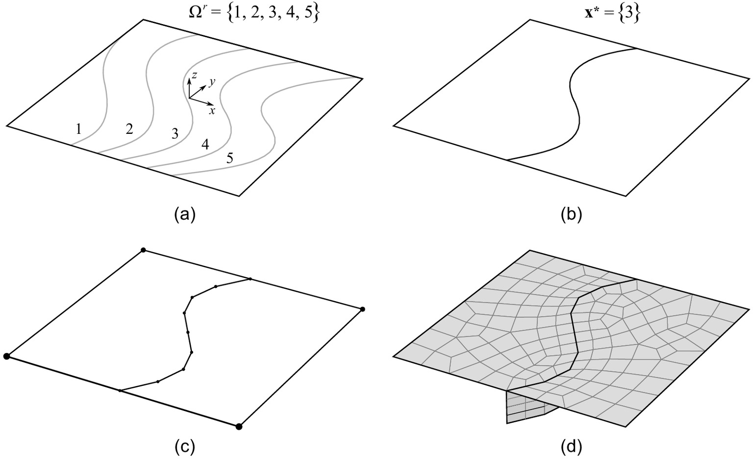
The FE model is generated through a series of geometric operations that are illustrated in Fig. 3. The slab is first subdivided into regions by setting one or more rib curve profiles depending on the candidate layout. The slab regions are then discretized into a series of shell elements using the Frontal Delaunay algorithm (Remacle, et al. 2010) from the Python library Gmsh (Geuzaine and Remacle 2009). At this stage, the slab thickness and rib cross-section dimensions [Fig. 2(a)] are kept constant. The slab thickness

t

is set to a predetermined minimum value (e.g., 40 mm). The depth of the ribs

d

is set so that the total depth of the floor system

(d + 0.5 t)

does not exceed a certain depth, which is determined based on typical dimensions for multistory buildings (e.g., 400 mm).

Fig. 3. Illustration of the FE model generation process: (a) solution domain $Ω^{r}$ ; (b) selection of solution set $x^{*}$ ; (c) curve discretization; and (d) rib extrusion and meshing.

At each iteration, all ribs in the candidate set

x^{cand}

are tested in combination with the ribs that are in the solution set

x^{*}

. The candidate set for the initial iteration is identical with

Ω^{r}

. In case no feasible configuration is obtained, the rib

x \in x^{cand}

having the minimum distance to the constraint boundary is added to the solution set

x^{*}

.

If multiple feasible configurations are obtained, the rib

x \in x^{cand}

causing the least deterioration of the objective function (i.e., the smallest increase in the volume of the slab-ribs assembly) is added to the solution set. Each time a rib

x^{*}

is added to the solution set

x^{*}

, it is removed from

x^{cand}

. The process repeats until the constraints in Eqs. (2a)–(2c) are satisfied.

After a rib layout is obtained, the slab thickness and rib cross-section sizing are optimized. For formulation and fabrication simplicity,

w

and

d

for all passive and active ribs are assumed to be identical. However, depending on the depth required to host the adaptive tensioning system, active ribs are typically deeper than passive ribs. In this formulation, the depth of the passive ribs is reduced by a factor

0 < β \leq 1

from that of the active ribs,

β d

. To further simplify the design variables

x = {[\begin{matrix} t & w & d \end{matrix}]}^{T}

, the rib width

w

is fixed to a predetermined ratio with respect to the slab thickness

t

(e.g.,

w / t = 2

). This ratio has been set to ensure minimum cover and sufficient space for the reinforcement and the tension cable. Combined with the limitation on the total depth of the floor system (e.g.,

d + 0.5 t = 400 mm

), the sizing optimization is formulated as a univariate problem with a design variable

x = t

. Because the objective function

V (x)

reduces monotonically with the value of

t

, the sizing optimization can be formulated as a minimization of the distance to the governing constraint boundary, which in this case is the displacement limit

\min_{x} (\max (| C d^{SLS, c} |) - \frac{l^{s}}{500})

(3)

which is solved through a univariate minimizer (Brent 1973) from the Python library SciPy (Jones et al. 2001).

It is assumed that the slabs are used in residential or office areas requiring a live load category of A and B according to Eurocode 2 (CEN 2010). In this work, live loads are nonsustained actions occurring for a period that is significantly shorter than the design life. The long-term deflection due to creep is estimated by magnifying the deflection under quasi-permanent load as

(1 + ψ) d^{SLS, \infty}

. In this case, a reduction factor of 0.3 for live loads is adopted as recommended by Eurocode 2 (CEN 2010). The creep coefficient

ψ

is computed by taking the following assumptions: (1) a relative humidity of 70% (based on an average measure in southwest Germany); and (2) because live loads have a long return period, it is extremely unlikely that peak loads occur at

t_{0} = 28

days, so the design load is assumed to occur not earlier than a concrete age of

t_{0} = 100

days. If the maximum compressive stress utilization exceeds 45%, the creep coefficient is magnified by

\exp (1.5 (ϕ - 0.45))

, where

ϕ

is the maximum compressive stress utilization. The long-term deflection criterion is met if

\max (| (1 + ψ) d^{SLS, \infty} |) \leq l^{s} / 250

.

Control Strategy

Controller Design

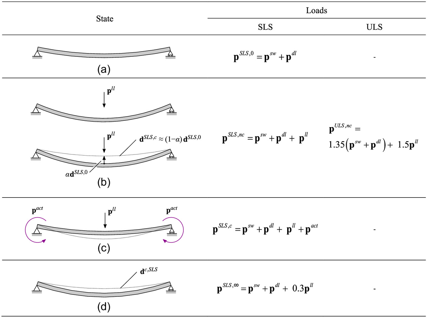
Fig. 4 gives an illustration of the main states of the structure during service, including the adaptation process. Fig. 4(a) shows the default state under permanent load (self-weight + superimposed dead load). Fig. 4(b) shows the noncontrolled state under the external load, and Fig. 4(c) shows the controlled state under the combined effect of external and actuation load. The superscript 0 generally refers to the non-controlled state, i.e., the response is caused by the effect of the external load only. Fig. 4(d) shows the long-term default state under quasi-permanent load (self-weight + superimposed dead load + reduced live load).

Fig. 4. Adaptation states and design limit states [load factors according to the Eurocode (CEN 2002)]: (a) default state, under permanent load; (b) deformed state, under load; (c) controlled state, under load; and (d) long-term default state, under quasi-permanent load.

The controller is designed to reduce deflections under loading to satisfy the required deflection criteria. Only static responses are considered, and thus the system is modeled as follows:

K d^{SLS, c} = p^{SLS} + p^{act}

(4)

where

K \in R^{n^{d} \times n^{d}}

is the global stiffness matrix of the structure;

d^{SLS, c} \in R^{n^{d}}

is the displacement caused by the combined action of the external load and actuation for the serviceability limit state; and

p^{SLS}

and

p^{act} \in R^{n^{d}}

are external and actuation loads (i.e., control input), respectively. In this case, the output

y

of the system, which is to be controlled, is the displacement of selected degrees of freedom:

y = C d^{SLS, c}

(5)

Because there are

n^{act}

active ribs, the control input

p^{act}

is a function of the cable tension

T \in R^{n^{act}}

. Introducing the term

p^{act} = D T

, Eq. (5) can be expanded as follows:

y = C K^{- 1} p^{SLS} + C K^{- 1} D T

(6)

The formulation of the control input matrix

D \in R^{n^{d} \times n^{act}}

, which transforms the cable tension

T

into the resulting forces applied to the slab-rib assembly, i.e., control input

p^{act} = D T

, is given in the section “Adaptive Tensioning System.” The cable tension is computed to reach a target displacement that is set using a linear function of the displacement caused by the external load, i.e.,

y = C d^{SLS, c} \approx (1 - α) C d^{SLS, 0}

. The cable tensions are computed by solving the unconstrained

L^{2}

-norm

{∥ C K^{- 1} D T + α C d^{SLS, 0} ∥}_{2}

for

T

T = - {(C K^{- 1} D)}^{+} α C \underset{d^{SLS, 0}}{\underset{⏟}{K^{- 1} p^{SLS}}}

(7)

For notation simplicity, the term

d^{SLS, 0} = K^{- 1} p^{SLS}

is introduced. Eq. (7) states that displacements caused by the control forces

C K^{- 1} D T

must be as close as possible to the displacement required to reach the target state, which is set to a fraction of the displacement caused by the external load

α C d^{SLS, 0}

. In this case, the target deflection after control is limited to

\max (| C d^{SLS, c} |) = l^{s} / 500

, and thus the scaling factor

α \in R

is

α = 1 - \frac{l^{s}}{500 \cdot \max (| C d^{SLS, 0} |)}

(8)

During control, the cable tension

T

is limited by the actuator capacity as well as the mechanical properties of the cable, and the controller [Eq. (7)] is modified to enforce an upper bound on

T^{\max}

as follows:

\min_{T} {∥ C K^{- 1} D T + α C d^{SLS, 0} ∥}_{2}

(9)

subject to

0 \leq T \leq T^{\max}

(10)

For clarity, if no solution can be obtained that meets the constraint on the tension force, all actuators are saturated, i.e.,

T

is a vector whose entries are all equal to the upper bound,

T_{i} = T^{\max} : \forall i = {1, 2, \dots, n^{act}}

, and is likely that the deflection limits cannot be met through control.

Adaptive Tensioning System

The transformation of the cable tension

T \in R^{n^{act}}

into control input

p^{act} \in R^{n^{d}}

is carried out through premultiplication by the control input matrix

D \in R^{n^{d} \times n^{act}}

, which collects columnwise the forces produced by the application of a unitary tensile force in the

m

th cable

D = [\begin{matrix} δ_{1} & \dots & δ_{m} & \dots & δ_{n^{act}} \end{matrix}]

(11)

The resulting or equivalent force on the structure

δ_{m} \in R^{n^{d}}

from the active tensioning of each cable is estimated through a numerical integration based on the two-point Gauss quadrature rule

δ_{m} = - \sum_{i = 1}^{2 n^{seg}} \sum_{j = 1}^{4} L_{h} \frac{l_{h}^{2} γ_{i}}{λ_{h}} (v_{i} v_{i}^{T}) J_{h i}^{- 1} {\begin{matrix} \frac{\partial N_{i j}}{\partial ξ} \\ \frac{\partial N_{i j}}{\partial η} \end{matrix}}; h = ⌈ \frac{i}{2} ⌉

(12)

Eq. (12) is formulated for active ribs with a straight axis and modeled with quadrilateral shell elements. Each rib has an

x - y

coordinate system originating from one of the two lower vertices. Each shell element in the active rib is considered a hosting element that has a local isoparametric

ξ - η

coordinate system originating from the center (0,0), where

- 1 \leq ξ \leq 1

and

- 1 \leq η \leq 1

. The cable is subdivided into

n^{seg} \in Z

segments according to how many shell elements it passes through. The subscript

h

,

\forall h = {1, \dots, n^{seg}}

, denotes the

h

th segment of the cable as well as the overlapping

h

th shell element. The subscript

i

,

\forall i = {1, \dots, 2 n^{seg}}

, indicates that the variable is evaluated at the

i

th integration point; there are two integration points for each cable segment, namely

{- 1 / \sqrt{3}, 1 / \sqrt{3}}

that correspond to

i = {2 h - 1, 2 h}

. The subscript

j

,

\forall j = {1, \dots, 4}

, denotes the

j

th node of the quadrilateral shell element that hosts the

h

th cable segment. The operator

⌈ \cdot ⌉

denotes a ceiling function, where

⌈ x ⌉ = \min {\bar{x} \in Z | \bar{x} \geq x}

.

L_{h} \in {0, 1}^{n^{d} \times 2}

is a matrix that maps the equivalent forces for each rib onto the corresponding structural degrees of freedom;

l_{h} \in R

and

λ_{h} \in R

are the length of the

h

th cable segment in global coordinates, and in the local (isoparametric) coordinate of the hosting element. Then,

v_{i} = {[\begin{matrix} v_{i x} & v_{i y} \end{matrix}]}^{T} = r^{'} (t) / ∥ r^{'} (t) ∥

is the normalized tangent vector of the cable evaluated at the

i

th integration point, and

r (t) = {[\begin{matrix} x (t) & y (t) \end{matrix}]}^{T}

is the cable placement profile expressed in a parametric form.

J_{h i} \in R^{2 \times 2}

is the Jacobian of the two-dimensional transformation between the

x - y

global coordinate and the

ξ - η

local coordinate of the shell element hosting the

h

th segment of the cable.

\partial N_{i k} / \partial ξ

and

\partial N_{i k} / \partial η

are the partial derivatives of the shape functions

N_{i} = {[\begin{matrix} N_{i 1} & N_{i 2} & N_{i 3} & N_{i 4} \end{matrix}]}^{T}

of the host element with respect to the local axes;

γ_{i} \in R

;

0 \leq γ_{i} \leq 1

is the factor of tension loss due to friction at the

i

th integration point based on an exponential decay function (CEN 2010)

γ_{i} = \exp {- μ ϖ l_{h} - μ \sum_{k = 1}^{i} \cos^{- 1} (\frac{v_{k}^{T} v_{k - 1}}{∥ v_{k} ∥ ∥ v_{k - 1} ∥})}; h = ⌈ \frac{i}{2} ⌉; \forall i = 1, \dots, 2 n^{seg}

(13)

where

μ

= static friction coefficient. The wobble factor

0.005 \leq ϖ \leq 0.01

is included to account for nonintended curvature caused by construction errors (CEN 2010), which also exists when the cable is straight, i.e.,

v_{k} = v_{k - 1}

;

\forall k = {1, \dots, i}

. Figs. 5(a and b) illustrate the indexing convention for Eqs. (12) and (13). The derivation of Eqs. (12) and (13) are given in Appendixes I and II, respectively.

Fig. 5. Resulting force distribution from cable tension: (a and b) coordinate systems and indexing convention; and (c) an example of the resulting distribution.

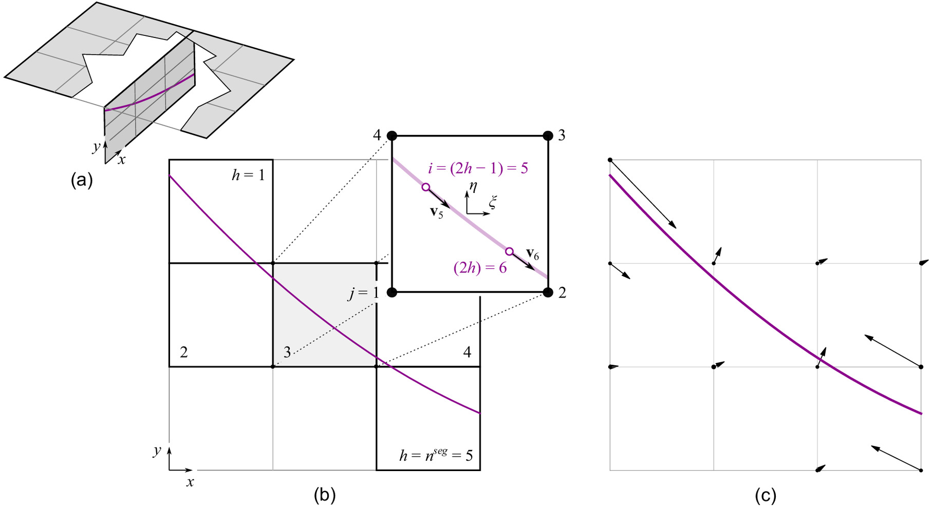
Figs. 5(c) and 6(a) show an example of the equivalent force distribution for a curved cable profile. Within the boundary of the structure, the forces act orthogonally to the cable. According to Eqs. (11) and (12), the orthogonal forces can be interpreted as off-balance force components that result from the variation of the direction of the cable tangent, i.e., a variation of the cable tension direction that can be employed to counteract the effect of the external load. At the boundary, the forces produced by the cable tension are tangential to the cable.

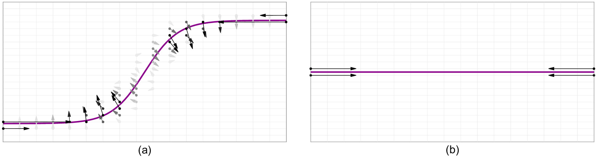
Fig. 6. Examples of resulting force distribution from cable tension: (a) curved cable; and (b) straight cable.

In case the cable is straight as shown in Fig. 6(b), the equivalent forces inside the domain are zero because they cancel at the interface of each shell element except those at the boundaries. Depending on the eccentricity of the cable axis to the slab-rib assembly axis, the overall effect is that produced by a negative moment, i.e., an upward bending that can also be employed to counteract the effect of the external load.

Case Study

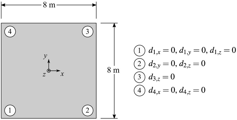
The method presented in the section “Design Method” has been applied to design an

8 \times 8 - m

adaptive rib-stiffened slab supported by four columns. The slab is assumed to be simply supported with boundary conditions illustrated in Fig. 7. In Support 1, translational movements are constrained in

x

-,

y

-, and

z

-directions. In Supports 2, 4, and 3 translational movements are allowed in

x

-,

y

-, and

x - y

-directions, respectively. The boundary condition was chosen to limit the complexity that arises from parasitic stresses that may occur in configurations with high degrees of redundancy. The slab is designed to take self-weight (SW) and live load (LL). SW is computed based on the volume of the structure assuming a 2,400 and

1,750 kg / m^{3}

density of concrete and rebars, respectively.

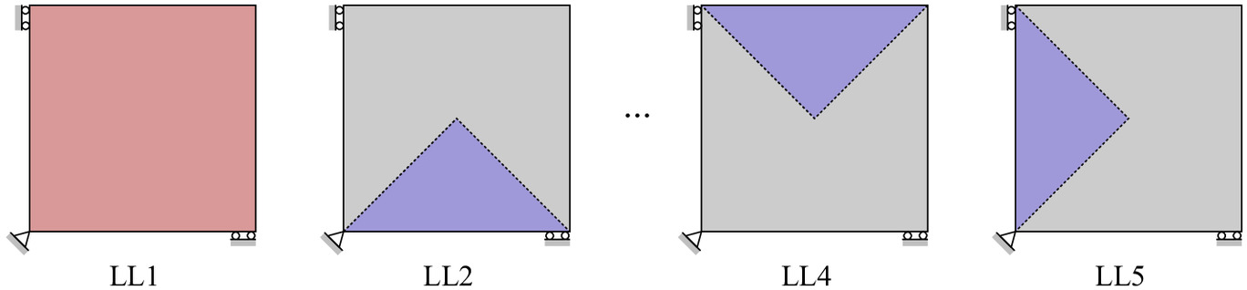
Fig. 7. Dimensions and boundary conditions.

As shown in Fig. 8, there are five live load patterns: LL1 is a uniformly distributed load of magnitude

3 kN / m^{2}

, and LL2 to LL5 are patch loads of magnitude

9 kN / m^{2}

applied anticlockwise to each of the four isosceles triangles formed by the two main diagonals. The magnitude of the patch loads has been set higher than that of the uniform load to evaluate the effect of asymmetrical actions on the control performance. In this case, it is of interest to investigate the control efficacy when the location of the maximum deflection is not directly above any active ribs. LL2 to LL5 are considered the worst cases for slabs supported by four columns according to the yield-line theory (Johansen 1962). Six load combinations were considered as summarized in Table 1.

Table 1. Load cases

Load case	Load combination
LC0	SW
LC1	SW + LL1
LC2	SW + LL2
LC3	SW + LL3
LC4	SW + LL4
LC5	SW + LL5

Because the stress utilization of the obtained solution is relatively high (e.g.,

\sim 0.5 f_{c}^{'}

), the slab was assumed to be made of

f_{c}^{'} = 50 MPa

concrete (C50/C60) with an estimated Young’s modulus of 37 GPa (CEN 2010) which is adequate to mitigate the long-term effects of creep as described in the section “Deflection and Stress Behavior.”

As a reinforcement, carbon fiber rebars were placed in the lower (tensile) region of the ribs, with a diameter of 10 mm and a concrete cover of 15 mm. Because the mechanical properties of carbon fiber vary greatly depending on material specifications, lower-bound values given in ACI 440.1R-15 (ACI Committee 2015) were used. Here,

f_{u}^{*} = 1863 MPa

was taken as the nominal rupture capacity of the rebars, which was reduced to

f_{u} = 0.5 f_{u}^{*} = 931 MPa

to account for long-term degradation. Carbon fiber-reinforced polymer (CFRP) rebars have been adopted to provide a feasible solution due to space limitations caused by significant concrete mass reduction. For example, the maximum rib width considered in this work is 80 mm. When the rib is active, it also houses the tension cable. If steel is adopted, the eccentricity of the cables with respect to the neutral axis must be reduced to fit an adequate concrete cover for anticorrosion measures.

The curve layout, shown in Fig. 9(a), is based on the directions of the principal stress caused by a uniformly applied load. The geometric construction of such a layout is carried out following a process described by Halpern et al. (2013). This curve layout is set as the solution domain

Ω^{r}

for the rib layout optimization (Section “Design Method”). The solution domain comprises 240 orthogonal curves. However, owing to the symmetry of the square configuration, the number of candidate ribs is reduced to 60. Fig. 9(b) shows the final rib layout configuration.

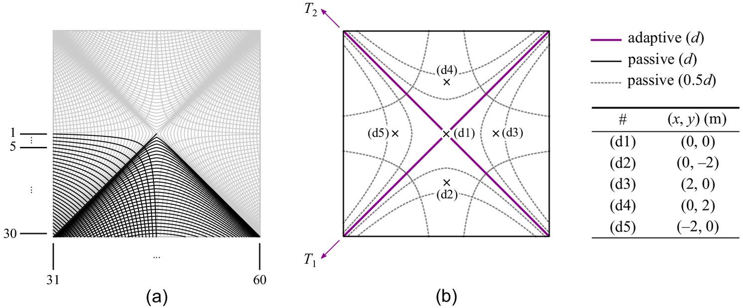
Fig. 9. (a) Solution domain $Ω^{r}$ ; and (b) rib layout, locations of observation points, and directions of control forces.

The diagonal cross ribs, indicated in continuous lines, are active ribs (

n^{act} = 2

) with a depth

d

. The required control forces

T = {[\begin{matrix} T_{1} & T_{2} \end{matrix}]}^{T}

were computed following the convention illustrated in Fig. 9(b). The four edge beams, indicated by solid lines, are passive ribs with a depth

d

. All other passive ribs, indicated by dashed curves, are assigned a depth

β d = 0.5 d

and are placed through the layout optimization process described in the section “Design Method.”

The slab thickness

t

(40 mm), rib width

w

(80 mm), and rib depth

d

(380 mm) [Fig. 2(a)] were obtained from sizing optimization (section “Design Method”). The total depth of the slab-ribs assembly was 400 mm

(d + 0.5 t = 400 mm)

.

The vertical degrees of freedom indicated by Points (d1)–(d5) in Fig. 9(b) were set as the controlled system output,

n^{c d} = 5

[Eq. (5)]. The controlled degrees of freedom were selected based on the estimated locations of the maximum displacement for each rib-layout configuration. Considering Load patterns LC1–LC5, regardless of the rib layout, the maximum displacement is expected to occur in the proximity of the centroid of each load pattern area.

The tension cable in the active rib was a steel strand with a nominal diameter of 48 mm (

A^{p} = 1,809.6 {mm}^{2}

) and Young’s modulus

E^{p} = 205 GPa

. The cable tension was assumed to be varied by an electromechanical actuator placed at one of the two ends of each active rib, indicated by arrows in Fig. 9(b). The tension loss

γ

in the cable (section “Adaptive Tensioning System”) was computed using a friction coefficient of

μ = 0.19

and a wobble factor (section “Adaptive Tensioning System”) of

ϖ = 0.005

assuming minimal alignment error resulting from fabrication (CEN 2010).

Benchmarking with Respect to Cable Profiles

As shown in Fig. 10, four cable profiles are benchmarked, namely, straight (S), parabolic (P), cosine (C), and super-Gaussian (SG). Cable profiles are expressed in a parametric form

r (t) = {[\begin{matrix} x (t) & y (t) \end{matrix}]}^{T}

, where

x (t) = t

and

y (t) = e^{p}

(14a)

y (t) = \frac{4 (e^{a} - e^{p}) t^{2}}{{(l^{r})}^{2}} + \frac{4 (e^{p} - e^{a}) y}{l^{r}} t + e^{a}

(14b)

y (t) = (e^{a} - e^{p}) \cos (\frac{2 π t}{l^{r}})

(14c)

y (t) = (e^{a} - e^{p}) [1 - 2 \exp {- {(\frac{2 t - l^{r}}{2 ζ})}^{2 q}}], q \in Z, 0 < ζ < 0.5 l^{r}

(14d)

for

0 \leq t \leq l^{r}

, where

l^{r} \in R

is the length of an active rib; and

e^{a} \in R

and

e^{p} \in R

is the cable elevations at the anchor and the apex, respectively. Four SG profiles were tested, namely SG1–DG4 obtained through Eq. (14d) by setting parameters

q \in {8, 3, 3, 1}

and

ζ \in {0.45 l^{r}, 0.375 l^{r}, 0.25 l^{r}, 0.125 l^{r}}

.

Fig. 10. Cable placement profiles: (a) straight (S); (b) parabolic (P); (c) cosine (C); and (d) super-Gaussian (SG).

Fig. 11 shows the variation of the average control forces

Σ T_{m} / n^{act}

required under LC1 for various cable profiles and anchor elevations

e^{a} \in {100, 200, 300, 360} (mm)

. Average values are presented because LC1 is a symmetric load case and thus

T_{1}

and

T_{2}

are not significantly different. Generally,

T_{1}

and

T_{2}

differ because the cables in the active ribs must meet with different elevations to avoid a collision, which generates an asymmetry in the control forces.

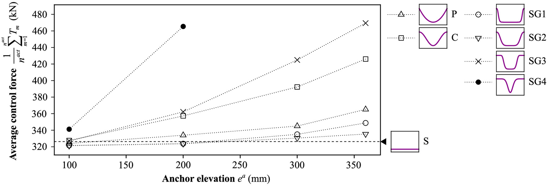
Fig. 11. Average of control forces under LC1 using various cable profiles and anchor elevation.

In this case, the apex elevation

e^{p}

of Active rib 1 was set to 50 mm, 100 mm lower than that for Active rib 2. A limit of

T^{\max} = 600 kN

on the control forces was enforced. The average control force for the straight (S) profile is indicated by a dashed horizontal line because the anchor elevation

e^{a}

is constant and identical with the apex elevation

e^{p}

.

The intensity of the control forces is also employed as a measure of control efficacy. Higher control efficacy is achieved when lower control forces are required to achieve the control objective. A comparatively uniform distribution of low-magnitude orthogonal forces is expected when the parabolic (P) and cosine (C) profiles are employed because the tangent directions do not vary significantly in this case. On the other hand, for the super-Gaussian (SG) profiles, higher-magnitude orthogonal forces are expected in the region where the cable tangent and curvature abruptly change direction, such as in SG1–SG4 profiles.

Results for SG3 and SG4 profiles show that drastic change of curvature in the center region of the rib generally resulted in poor control efficacy, especially when

200 \leq e^{a} (mm)

. Similarly, P and C profiles gave lower control efficacy although changes of curvature were less drastic. On the other hand, when the curvature change was localized at the extremities of the rib, such as in SG1 and SG2 profiles, control efficacy was generally high. For all profiles, higher control efficacy was obtained when the elevation

e^{a}

of the anchor was kept low. The active ribs considered in this work are relatively shallow (

d = 380 mm

) because in practice the total slab depth must be limited to within 400 mm. For this reason, the effect of the bending moment caused by the compressive forces at rib ends dominates over that of the orthogonal forces that develop by tensioning the cable (section “Adaptive Tensioning System”). Except for the SG4 profile, the variation in control forces when

e^{a} = 100 mm

was marginal, with SG2 giving the highest control efficacy.

Benchmarking with Respect to Active Rib Layouts

Three active rib layouts have been tested as illustrated in Fig. 12. In Layouts 1 and 2,

n^{act} = 2

diagonal cross ribs and

n^{act} = 4

edge ribs are active, respectively. Layout 3 is a combination of Layouts 1 and 2, resulting in a total of

n^{act} = 6

active ribs.

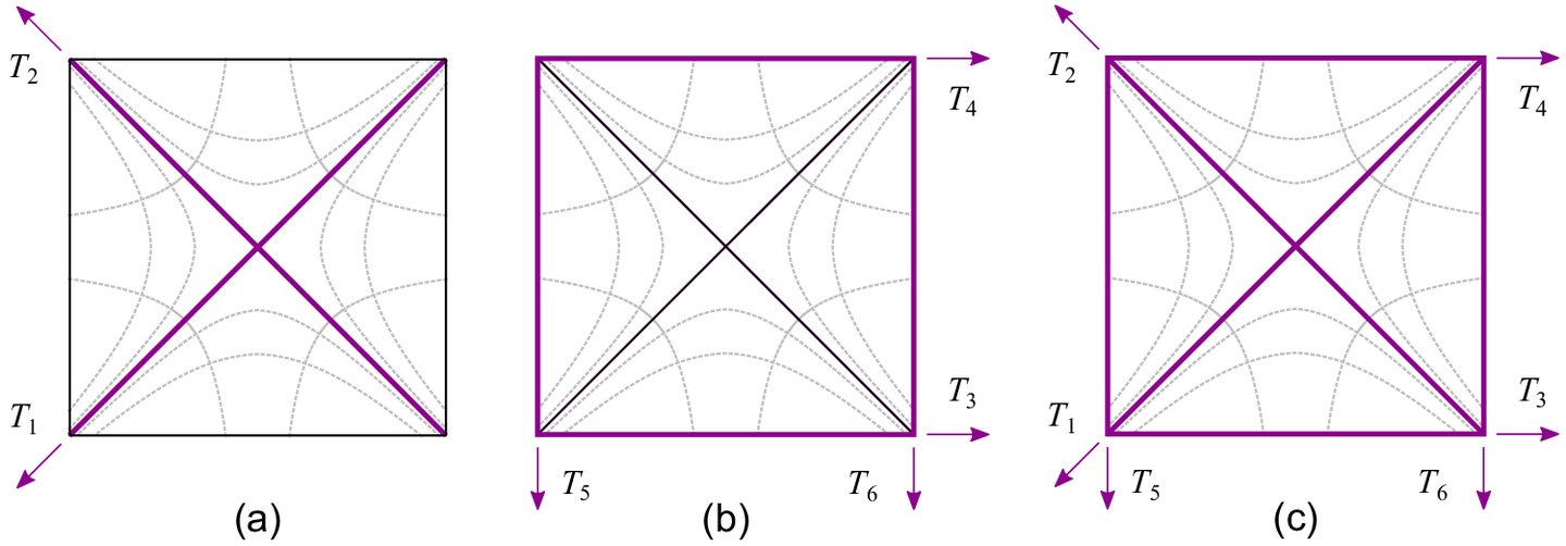
As given in Table 2, the cables of Active ribs 1 and 2–6 were placed following the SG2 and S profiles, respectively. Similar to section “Benchmarking with Respect to Cable Profiles,” the apex elevation

e^{p}

of Active rib 1 was set to 50 mm, 100 mm lower with respect to Active rib 2 to avoid collision between the two crossing cables. To provide room for the actuators, the anchor elevation

e^{a}

for Active ribs 1–2, 3–4, and 5–6 are offset at 100, 50, and 150 mm, respectively. The control forces

T^{\max}

for Layouts 1, 2, and 3 are limited to 400, 300, and 150 kN, respectively, to obtain solutions that can be implemented using standard actuators (e.g., electromechanical and hydraulics).

Table 2. Cable profile, cable elevation, and required control forces

Active rib	Cable profile	Cable elevation (mm)		Control force, $T_{m}$ (kN)
		Cable elevation (mm)		Layout 1			Layout 2			Layout 3
		$e^{a}$	$e^{p}$	LC1	LC2	LC3	LC1	LC2	LC3	LC1	LC2	LC3
1	SG2	100	50	320	81	400^a	—	—	—	150^a	150^a	150^a
2	S	100		323	400^a	9	—	—	—	150^a	150^a	150^a
3	S	50		—	—	—	202	300^a	134	123	150^a	52
4	S	50		—	—	—	202	52	85	123	0	0
5	S	150		—	—	—	258	166	136	150^a	0	66
6	S	150		—	—	—	258	108	300^a	150^a	60	150^a

a

Saturated active rib;

T_{m} = T^{\max}

.

For brevity, results for LC4 and LC5 are not presented because they mirror LC2 and LC3, respectively. Although the configuration of the adaptive rib-stiffened slab is symmetric, the control forces in the two tensioning cables

(T_{1}, T_{2})

are not identical, even under symmetric loads (e.g., LC1). The difference between the two tensioning cables can be attributed to (1) the difference in terms of the apex elevation (Table 2), (2) asymmetric application of the control force because only one actuator per active rib is employed [Fig. 9(b)], and (3) asymmetric boundary conditions (Fig. 7).

Table 3 gives the absolute values of the maximum displacements in the uncontrolled

| d^{SLS, 0} |

and controlled

| d^{SLS, c} |

states observed at Points d1–d5 [Fig. 9(b)]. In the uncontrolled case, the deformation limits

l^{s} / 500 = 16 mm

were never satisfied. A maximum displacement of 27 mm occurred at Point d1 under LC1. With Layout 1, one out of

n^{act} = 2

actuators was saturated, and the displacement limit was always satisfied through control. With Layout 2, although only one out of

n^{act} = 4

actuators was saturated under LC2 and LC3, the serviceability limits of 16 mm cannot be satisfied if the control forces are limited to

T^{\max} = 300 kN

. This occurs because none of the active ribs was placed in the proximity of the controlled degrees of freedom, resulting in low-efficacy actuators. Because Layout 3 has more actuators, serviceability limits were satisfied under all cases with a lower control force limit

T^{\max} = 150 kN

.

Table 3. Displacements before and after control

Observation point	Displacements before control, $\| d^{SLS, 0} \|$ (mm)			Displacements after control, $\| d^{SLS, c} \|$ (mm)
	Displacements before control, $\| d^{SLS, 0} \|$ (mm)			Layout 1			Layout 2			Layout 3
	LC1	LC2	LC3	LC1	LC2	LC3	LC1	LC2	LC3	LC1	LC2	LC3
(d1)	27^a	22^a	22^a	16	15	15	16	15	15	16	15	15
(d2)	23^a	24^a	18^a	14	16	12	14	17^a	12	13	16	12
(d3)	23^a	18^a	24^a	14	12	16	14	12	17^a	14	12	16
(d4)	23^a	17^a	17^a	14	11	11	14	11	12	13	11	12
(d5)	23^a	17^a	17^a	14	11	11	14	12	11	14	12	11

a

Deformation exceeding

l^{s} / 500 = 16 mm

limits.

Deflection and Stress Behavior

A configuration based on active rib Layout 3 [Fig. 12(c)] is studied in further detail from hereafter. Fig. 13 shows the gradient map of the vertical displacements under LC1–LC3 overlaid onto the planar view of the adaptive rib-stiffened slab. The uncontrolled displacements caused by the external load are shown in Figs. 13(a–c), and those caused by the controlled state in Figs. 13(d–f), respectively. A darker shade of gray indicates a greater displacement, and regions where the limit

l^{s} / 500 = 16 mm

is exceeded are also indicated.

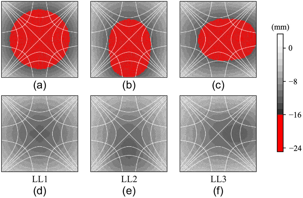
Fig. 13. Vertical displacements: (a–c) uncontrolled state; and (d–f) controlled state.

Fig. 14 shows the gradient map of the minimum principal stress (i.e., maximum compressive stress) observed at the uppermost region of the slab structure under LC1–LC3. Stress fields for the uncontrolled [Figs. 14(a–c)] and controlled [Figs. 14(d–f) cases are shown, respectively]. Fig. 15 shows the axial stress in the rebars under LC1–LC3.

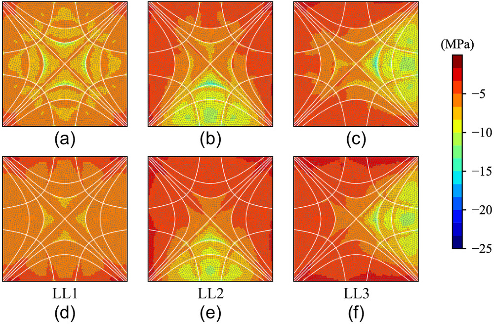
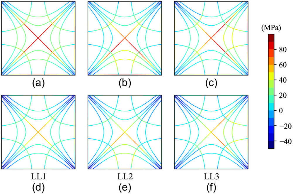
Fig. 14. Minimum principal stress on the uppermost fiber: (a–c) uncontrolled state; and (d–f) controlled state.

Fig. 15. Rebar stress: (a–c) uncontrolled state; and (d–f) controlled state.

Table 4 gives a summary of compressive stresses in the concrete slab and tensile stresses in the rebars. A metric of stress utilization

ϕ

is employed to indicate the percentage ratio between the observed stress and the material stress capacity. The compressive stress utilization was computed based on the compressive capacity of the concrete slab-ribs assembly,

f_{c}^{'} = 50 MPa

. Because the concrete tensile capacity is neglected, the tensile stress utilization was computed based on the tensile capacity of the carbon fiber rebar,

f_{u} = 931 MPa

. Therefore

ϕ = {\begin{matrix} - \min (σ) / f_{c}^{'} \\ \max (σ) / f_{u} \end{matrix}

(15)

Table 4. Maximum stress demand before and after control

Stress demand, $ϕ$	Before control (%)			After control (%)
Stress demand, $ϕ$	LC1	LC2	LC3	LC1	LC2	LC3
Concrete slab, upper fiber, cs	20 ^(cs1–4)	27 ^(cs1)	27 ^(cs2)	18 ^(cs1–4)	21 ^(cs1)	22 ^(cs2)
Concrete ribs, anchor area, cr	18 ^(cr1,2)	46 ^(cr1)	36 ^(cr2)	33 ^(cr1)	49 ^(cr1)	39 ^(cr2)
Carbon fiber rebars, r	8 ^(r1)	9 ^(r2,3)	9 ^(r4,5)	6 ^(r1)	7 ^(r6,7)	7 ^(r7,8)

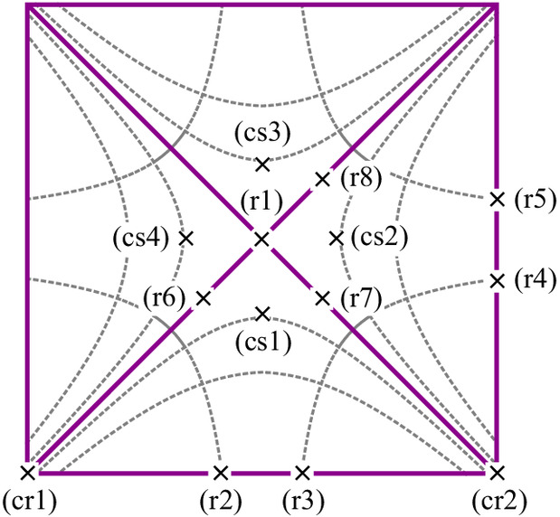
Note: Superscript indicates location of maximum stress demand as per Fig. 16.

Referring to Table 4, the compressive stress utilization in the slab (cs) and ribs (cr), as well as the rebar stress utilization (r), are given separately. Following the same naming conventions, the respective locations for the maximum stress are indicated in Fig. 16.

Under LC1 before control, a maximum compressive stress utilization of 20% occurred in the upper fiber of the slab at Points cs1–cs4. In the controlled case, the stress utilization reduced to 18%. In the anchor area of the rib at Points cr1,2, the stress increased significantly through control, resulting in 33% utilization compared with 18% for the uncontrolled case. Similarly, in the anchor area of the rib at Points cr1, an increase in stress utilization from 46% to 49% occurred through control under LC2. In the upper region of the slab at Points cs1, stress utilization reduced from 27% to 21% through control. The increase in compressive stress around the anchor area can be attributed to the compressive effects from the cable ends. As illustrated in Fig. 14, the application of control forces

T

resulted in a pair of compressive forces at the ends of the cable. Overall, through active control of deflections, compressive stresses reduced in the slab and increased in the ribs.

In terms of the rebar tensile stress, the maximum tensile stress utilization reduced from 8% to 6% through control under LC1. In both cases, the maximum tensile stress occurred at Point r1, where the two cross-diagonal ribs intersect. In the uncontrolled case under LC2, the maximum tensile stress occurred in the edge rib that is in direct proximity to the patch load, specifically at Points r2 and r3. In the controlled case, the location of maximum tensile stress moved to Points r6 and r7. In this case, the maximum tensile stress utilization reduced from 9% to 7% through control.

Similarly, under LC3, the maximum tensile stress occurred at Points r4 and r5 in the uncontrolled case, and then moved to Points r7 and r8 in the controlled case. Because the rebars were placed in the lower region, they were primarily in tension in the uncontrolled state. However, the rebars are in compression in proximity to the supports in the controlled state due to the compressive forces generated by tensioning the cable. Although the adaptive solution might not be the global optimum (Section “Discussion”), improvement in material utilization is limited by load factors that must be considered for ULS states. However, the stress utilization in the upper fiber under the uncontrolled state improved by up to 9% and 6% compared with the equivalent rib-stiffened slab and passive flat slab, respectively.

Although the tension in the lower fiber of the ribs reduced significantly through control, tensile stress, and thus cracks, in the controlled state are allowed in the formulation given in the section “Design Method.” The formation of cracks reduces the effective concrete cross section, thereby redistributing the tensile stress to the reinforcement. In this case, the ultimate resistance of the structure is outside the linear-elastic domain. However, the effect of cracks is not explicitly considered in the formulation to limit optimization complexity.

Criteria for the ultimate state provided in design codes typically limit the compressive strain in the upper fiber to 0.0035 under uniaxial bending. Although the adaptive rib-stiffened slab in this study is subjected to biaxial bending, the ribs resist external loads predominantly through uniaxial bending because the configuration is obtained through a heuristic based on principal stress directions. To evaluate this criterion, a loss of stiffness was simulated by not accounting for the effect of the rebars in the lower region, and the response was computed under the ULS load. The uncontrolled maximum compressive strains in the upper fiber are below the crushing strain limit of 0.0035, namely

2.35 \times 10^{- 4}

,

2.91 \times 10^{- 4}

, and

2.94 \times 10^{- 4}

under LC1, LC2, and LC3, respectively.

In terms of long-term deflection, the effect of creep was estimated by magnifying the deflection under quasi-permanent load cases as

(1 + ψ) d^{SLS, \infty}

. Using assumptions given in the section “Design Method,” a basic creep coefficient

ψ = 1.11

was obtained. Because the maximum compressive stress utilization reached 49% under LC2, a nonlinear creep coefficient

ψ = 1.11 \cdot \exp (1.5 (0.49 - 0.45)) = 1.18

was used under LC2. The absolute values of the maximum long-term displacements

| (1 + ψ) d^{SLS, \infty} |

were 32, 30, and 29 mm under LC1, LC2, and LC3, respectively, and therefore the criterion for long-term deflection is satisfied (

l^{s} / 250 = 32 mm

).

Mass and Energy Assessment

The adaptive rib-stiffened slab was benchmarked against an equivalent mass-optimized passive rib-stiffened slab, a passive flat slab, and a passive voided slab. The sizing of the passive slabs was optimized using the same formulation as in Eqs. (1) and (2), excluding the constraint on the control forces [Eq. (2c)] and adding a constraint that limits the maximum displacement to

l^{s} / 500

. The rib layout of the passive rib-stiffened slab was identical with that of the adaptive rib-stiffened slab. The resulting passive rib-stiffened slab had dimensions of 110 mm (

t

), 220 mm (

w

), and 345 mm (

d

). The total depth was

d + 0.5 t = 400 mm

. The passive rib-stiffened slab was not post-tensioned.

Because loads were assumed to have a long-return period, long-sustained stress due to post-tensioning might cause several problems including unwanted permanent stress and might accelerate creep-related issues. In addition, through conventional post-tensioning, there will be a loss of tension in the cable, potentially causing violation of the serviceability limit state. On the contrary, for the adaptive configuration, cable tensioning was applied when needed. For this reason, a benchmark with a post-tensioned passive rib-stiffness slab would not be significant.

The equivalent mass-optimized passive flat slab had a thickness

t

of 275 mm. For the equivalent passive voided slab, it was assumed that hollow spheres are employed. Following a design method for voided slabs given by Schmeer (2021), a 35% reduction in concrete volume was predetermined. Compared with a conventional flat slab with identical total thickness, this volume reduction corresponds approximately to a 10% loss in flexural stiffness, and thus a reduction of Young’s modulus in the same proportion (Fanella et al. 2017; Schmeer and Sobek 2018; Nigl et al. 2022). A passive voided slab with a total thickness

t

of 250 mm was obtained.

For the adaptive rib-stiffened slab, the actuator mass was estimated through the product of the maximum required force with a proportional constant of

0.1 kg / kN

(ENERPAC 2016). As indicated in Table 5, the adaptive rib-stiffened slab achieved 50%, 59%, and 67% material mass savings with respect to the passive voided slab, passive rib-stiffened slab, and passive flat slab, respectively.

Table 5. Mass and energy benchmark: adaptive versus passive

Metric	Flat−passive (Case 1)	Rib-stiffened−passive (Case 2)	Voided−passive (Case 3)	Rib-stiffened−adaptive (Case 4)
Mass of reinforced concrete (t)	44	35.1	28.5	14.3
Mass of actuators + cables (t)	0	0	0	0.8
Mass savings (%)
With respect to Case 1	—	20	35	67
With respect to Case 2	—	—	19	59
With respect to Case 3	—	—	—	50
Active hours	0	0	0	6,249
$E^{e m}$ (MJ)	$6.614 \times 10^{5}$	$5.279 \times 10^{5}$	$4.284 \times 10^{5}$	$2.326 \times 10^{5}$
$E^{o p}$ (MJ)	0	0	0	$0.581 \times 10^{5}$
$E^{e m} + E^{o p}$ (MJ)	$6.614 \times 10^{5}$	$5.279 \times 10^{5}$	$4.284 \times 10^{5}$	$2.907 \times 10^{5}$
Energy savings (%)
With respect to Case 1	—	20	35	56
With respect to Case 2	—	—	19	45
With respect to Case 3	—	—	—	32

The embodied energy

E^{e m}

is the share of total energy embodied in the structural and actuation system. Based on data from the ÖKOBAUDAT database (Ministry for Housing, Urban Development and Building, Federal Republic of Germany 2013), the embodied energy associated with the structural system was obtained through the product of the total mass of reinforced concrete with a material energy intensity of

15 MJ / kg

. For a conservative estimation, it was assumed that actuators and tensioning cables are entirely made of nonrecycled primary steel with a material energy intensity of

35.4 MJ / kg

.

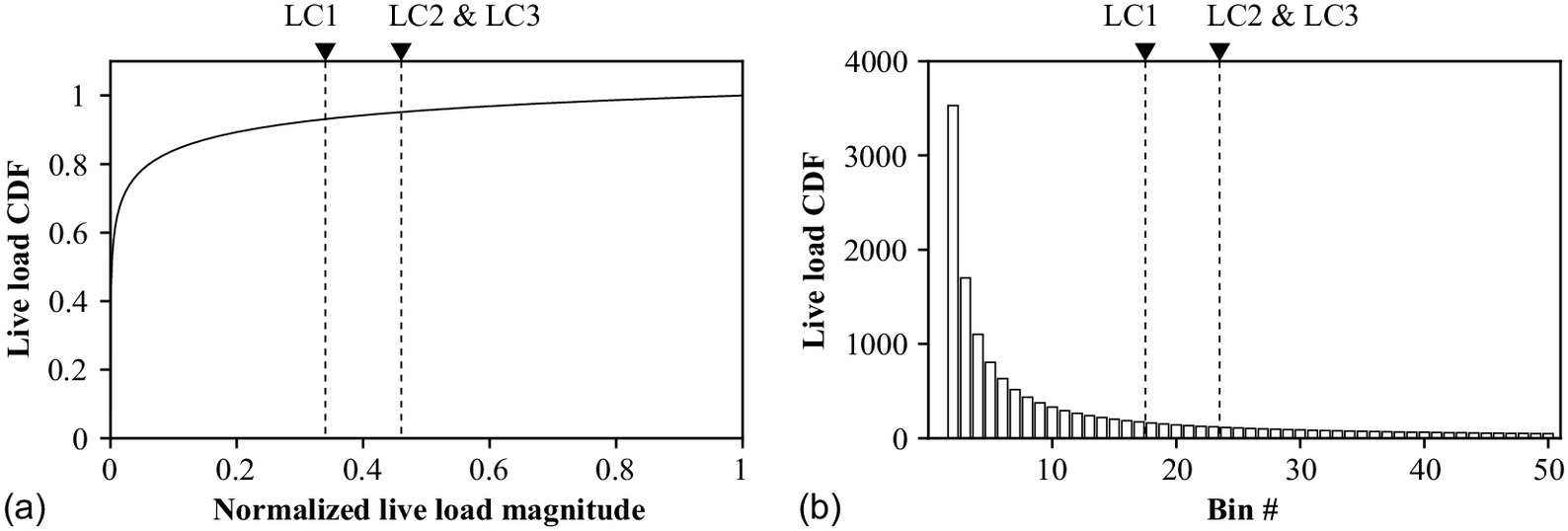
To estimate the operational energy

E^{o p}

, the live load magnitude was assumed to be distributed according to a lognormal function (Senatore et al. 2019). This means that the logarithm of the live load event is normally distributed. In this case,

p^{l l}

was set as the characteristic value, which corresponds to the 95th percentile of the associated normal distribution. The probability distribution function has been discretized into

n^{b} = 50

bins, i.e., 50 discrete load occurrences. The service life of the slab was set to 50 years.

Fig. 17 shows the live load cumulative distribution function (CDF) and the duration of the live load occurrence. The vertical dashed lines in Fig. 17 indicate the magnitude corresponding to the load activation threshold (LAT). The LAT is the highest loading intensity that the structure can take without adaptation (Senatore et al. 2019). The LAT criterion was set to

l^{s} / 500 = 16 mm

displacement limits. The vertical dashed lines in Fig. 17 indicate the magnitudes corresponding to LATs of

0.34 p^{l l}

under LC1 and

0.46 p^{l l}

under LC2 and LC3. The total number of active hours during which deflection control is required is 4,415.

L \subseteq {1, \dots, n^{b}}

is a set containing indices of bins that correspond to loads of magnitude larger than the LAT. Adopting the formulation given by Senatore et al. (2019), the operational energy

E^{o p}

is computed as follows:

E^{o p} = \sum_{m = 1}^{n^{act}} \sum_{l \in L}^{n^{b}} (\frac{w_{m l} Δ t_{l}}{η} \frac{ω}{2 π}); w_{m l} = \frac{T^{\min} + T_{m l}}{2} \underset{Δ l_{m l}}{\underset{⏟}{\frac{T_{m l} l_{m}^{p}}{E^{p} A^{p}}}}

(16)

where

w_{m l}

= work performed by the

m

th actuator to counteract the

l

th load occurrence through the application of the required total force

T_{m l}

. It was assumed that to perform deflection control [from the state in Fig. 4(b) to that in Fig. 4(c)], the actuators apply tensile forces linearly from a minimum magnitude

T^{\min} = 10 kN

to the required total force

T_{m l}

.

Fig. 17. (a) Live load CDF; and (b) duration of live load occurrence. LAT (indicated by solid triangles) is set to the deflection limit of $l^{s} / 500$ .

The magnitude of length changes (i.e., actuator strokes)

Δ l_{m l}

was estimated as the strain in the cable, which was computed through the multiplication of the total forces

T_{m l}

with the reciprocal of the axial stiffness of the cable

l_{m}^{p} / (E^{p} A^{p})

. In this case, the work

w_{m l}

is the area of a trapezoid with heights

(T^{\min}, T_{m l})

and width

Δ l_{m l}

. To compute the operational energy, it is assumed that the working frequency is equal to the fundamental frequency of the slab

ω / 2 π = 5.9 Hz

and the actuator mechanical efficiency is

η = 0.8

. It is assumed that no energy is needed to return to the default state after the load is removed [Fig. 4(a)] because this process involves a gradual release of tension in the cables.

Table 5 gives the whole-live energy assessment. Energy savings of 32%, 45%, and 56% were achieved with respect to the passive voided slab, passive rib-stiffened slab, and the passive flat slab, respectively.

Equivalent Carbon Assessment

The equivalent carbon (

{kgCO}_{2}

-equivalent) was computed by assuming that the slab is built in southwest Germany. Based on data from the ÖKOBAUDAT database (Ministry for Housing, Urban Development and Building, Federal Republic of Germany 2013), carbon equivalent metrics of 1.2 and

0.47 {kgCO}_{2} - eq. / kg

were taken to compute the total carbon footprint generated from fabrication and transport of the reinforced concrete slab and the actuation system, respectively.

The current energy mix for electricity generation (year 2022) causes approximately

0.4 {kgCO}_{2} - eq. / kWh

of greenhouse emissions (Energie Baden-Württemberg 2022). It has been estimated (European Environment Agency 2022) that the use of renewable sources is expected to increase significantly in the year 2050 to a proportion where electricity generation will cause

0.2 {kgCO}_{2} - eq. / kWh

of greenhouse emissions. Table 6 gives the equivalent carbon assessment based on the energy mix in the year 2022. The adaptive solution achieved up to 33%, 46%, and 57% reductions in carbon equivalent compared with the passive voided slab, passive rib-stiffened slab, and passive flat slab, respectively. Assuming that the target for the renewable energy mix will be achieved by the year 2050 (Table 7), the equivalent carbon can be further reduced by up to 42%, 53%, and 63% compared with the passive voided slab, passive rib-stiffened slab, and the passive flat slab, respectively.

Table 6. Equivalent carbon benchmark adaptive versus passive for 2022 energy mix in southwest Germany

Metric	Flat−passive (Case 1)	Rib-stiffened−passive (Case 2)	Voided−passive (Case 3)	Rib-stiffened−adaptive (Case 4)
$C O^{e m}$ ( ${kgCO}_{2} - eq$ )	$5.308 \times 10^{4}$	$4.236 \times 10^{4}$	$3.437 \times 10^{4}$	$1.662 \times 10^{4}$
$C O^{o p}$ ( ${kgCO}_{2} - eq$ )	0	0	0	$0.646 \times 10^{4}$
$C O^{e m} + C O^{o p}$ ( ${kgCO}_{2} - eq$ )	$5.308 \times 10^{4}$	$4.236 \times 10^{4}$	$3.437 \times 10^{4}$	$2.308 \times 10^{4}$
Carbon reductions (%)
wrt. Case 1	—	20	35	57
wrt. Case 2	—	—	19	46
wrt. Case 3	—	—	—	33

Source: Data from Energie Baden-Württemberg (2022).

Table 7. Equivalent carbon benchmark adaptive versus passive for 2050 energy mix according to the EU projection

Metric	Flat−passive (Case 1)	Rib-stiffened−passive (Case 2)	Voided−passive (Case 3)	Rib-stiffened−adaptive (Case 4)
$C O^{e m}$ ( ${kgCO}_{2} - eq$ )	$5.308 \times 10^{4}$	$4.236 \times 10^{4}$	$3.437 \times 10^{4}$	$1.662 \times 10^{4}$
$C O^{o p}$ ( ${kgCO}_{2} - eq$ )	0	0	0	$0.323 \times 10^{4}$
$C O^{e m} + C O^{o p}$ ( ${kgCO}_{2} - eq$ )	$5.308 \times 10^{4}$	$4.236 \times 10^{4}$	$3.437 \times 10^{4}$	$1.985 \times 10^{4}$
Carbon reductions (%)
wrt. Case 1	—	20	35	63
wrt. Case 2	—	—	19	53
wrt. Case 3	—	—	—	42

Source: Data from European Commission (2016).

Discussion

The methodology presented in this work provides a solution for an early-stage design that can be further elaborated through appropriate detailing. Labor and other activities that affect monetary costs are important aspects. To keep the optimization reasonably simple, these aspects are not included in the formulation. Fabrication costs depend significantly on the type of adopted technology, and the cost of labor hours is typically specific to a particular region or country. In addition, considering the ongoing and future material scarcity and the advent of robotic fabrication, it is reasonable to assume that fabrication costs will be a fraction of the total construction cost. Material costs and potential additional costs associated with taxation on embodied carbon and global warming potential are likely to become dominant. Therefore, the solution for the adaptive floor system proposed in this work is likely to become a competitive solution. The examples discussed in the section “Case Study” have shown the methodology proposed in this work can produce practical solutions. For example, the solution proposed for the

8 \times 8 - m

slab requires only six actuators with a force capacity of 150 kN, which can be applied by standard actuators. This reduces significantly the control system complexity and indirectly the associated monetary costs.

To limit the formulation complexity, the effect of plasticity caused by tensile cracks was not explicitly considered in the optimization method. Instead, a 0.0035 compressive strain criterion from Eurocode 2 (CEN 2010) was evaluated after optimization (section “Deflection and Stress Behavior”). This criterion is typically used for beams and one-way slabs. However, because the ribs are resisting external actions predominantly through uniaxial bending, it is possible to evaluate the compressive strain and assess if the crushing strain limit is satisfied in the upper fiber.

The shear in the ULS state at the supports is assumed to be compensated by a thicker column head. Typically, it is desirable to thicken the slab in the proximity of the columns so that the thickness is at least equal to the height of the secondary ribs, which simplifies construction. This assumption was taken because the sizing of the columns depends on the building configuration, which is out of the scope of this work.

Because the analysis of continuous structures such as plates and shells is generally more complex compared with discrete systems such as trusses and frames, the total energy has not been explicitly formulated as the objective function as done in previous work (Wang and Senatore 2020). That being said, the energy and carbon appraisals (with global warming potential) that compare the adaptive with equivalent passive solutions give a good indication of the benefits that could be gained after mainstream adoption.

The rib layout optimization process presented in the section “Design Method” has been formulated as a combinatorial problem. Although several noncombinatorial approaches for rib placement have been proposed in previous studies (Afonso et al. 2000; Lam and Santhikumar 2003; Khosravi et al. 2007; Li et al. 2021), the resulting configurations generally involve complex geometries (e.g., nonprismatic ribs) and thus are difficult to fabricate. Through the proposed approach, configurations comprising prismatic ribs with a rectangular section can be obtained, thereby facilitating the integration of adaptive tensioning systems.

The combination of a greedy algorithm and heuristics based on the direction of principal stresses enables efficient solving of the combinatorial rib layout optimization problem. Taking the case study in the section “Case Study” as an example, there are 60 candidate ribs in the solution domain

Ω^{r}

. The rib placement process in the section “Design Method” is treated as a binary no-rib/rib problem for each candidate rib such that there are

2^{60} = 1.15 \times 10^{18}

possible solutions. On an Intel Core 17 3.60 GHz processor, the evaluation of a single candidate solution took approximately 240 s. A full enumeration of all possible combinations thus would take at least

8.77 \times 10^{12} years

to complete. For this reason, the global optimality of the solution can neither be guaranteed nor verified. By employing a greedy algorithm, a local minimum was obtained after 180 evaluations, which took approximately 12 h to complete. Although the final configuration is not guaranteed to be a global optimum, it gives 50%, 59%, and 67% mass savings compared with a passive voided slab, passive rib-stiffened slab, and the passive flat slab, respectively.

Results from the cable profile benchmark given in the section “Benchmarking with Respect to Cable Profiles” show that higher control efficacy can generally be achieved using a lower anchor elevation. This suggests that because the ribs are relatively shallow, the orthogonal forces caused by the change of cable curvature are not dominant. Instead, the compressive forces generated by tensioning the cable result in a moment that counteracts effectively the effect of the external load. As shown by the controlled responses in terms of stress (section “Deflection and Stress Behavior”), the compressive forces at the cable end cause a high utilization around the support area, which should be mitigated through adequate reinforcement detailing. Curvilinear ribs are not considered feasible candidates for active ribs because the integration of adaptive tensioning in curvilinear ribs generates undesired torsional effects and lateral forces perpendicular to the rib axis (Campbell and Chitnuyanondh 1975).

There are only six straight ribs in the solution domain

Ω^{r}

(two cross-diagonals and four edges), and thus the placement of active ribs was obtained by evaluating the performance of three symmetric layouts made of straight ribs on the control of the slab displacements. Results from the active rib layout benchmark given in the section “Benchmark with Respect to Active Rib Layouts” show that target displacement reduction can be achieved exactly when active ribs pass in proximity of the controlled degrees of freedom, i.e., when active ribs are placed in the two cross-diagonals. However, control forces up to 400 kN are required in this case. When the active ribs are placed in the cross-diagonals and the edges, the required control forces reduce to a more practical magnitude of 150 kN.

Compensation of dynamic responses (e.g., due to footfall) using the proposed system is feasible provided that the actuators can generate the required control forces at a frequency that match at least the first eigenfrequency of the slab. For example, the eigenfrequency of the

8 \times 8 - m

slab is 5.9 Hz. Because walking pace frequencies are typically within the range of 1.8–2.2 Hz, the slab studied in this work is not susceptible to the first and second harmonics of the excitation frequency. In this case, the maximum response due to footfall is likely to be significantly lower than the maximum static deflection (

\sim 10 mm

) that the proposed adaptive system is designed to compensate for. Therefore, the required magnitude of control forces for vibration control is likely to be significantly lower than that for static deflection control. Future work could look into extending the methodology to include dynamic effects.

Conclusion

A new method to design adaptive rib-stiffened concrete slabs is presented in this paper. A rib layout optimization process employing heuristics based on the principal stress directions has been formulated. A search method based on a greedy algorithm was proposed to solve the combinatorial problem for rib layout optimization. A control strategy based on a variable post-tensioning system integrated inside the ribs is employed. The deflection of the slab is reduced by adjusting the cable tensile force that is computed through a quasi-static controller based on constrained least-square optimization. A closed-form relationship between the cable tension and the response of the structure has been presented. Results from numerical simulations lead to the following conclusions:

•

The proposed method produces an adaptive rib-stiffened slab that satisfies safety criteria without the contribution of the active system, and serviceability limits are satisfied through active control.

•

Displacements are controlled within an acceptable margin of error (

\pm 0.5 mm

).

•

Displacement control reduces tensile stress by increasing compression, which is the desired behavior in concrete structures.

•

The required control forces can be kept below a practical threshold (

< 200 kN

).

•

The adaptive rib-stiffened slab achieves up to 67% material mass savings as well as 56% total energy savings compared with a flat slab.

•

The adaptive rib-stiffened slab achieves up to 57% equivalent carbon reductions assuming a typical energy mix for electricity generation.

Further investigation is necessary to confirm the feasibility of the proposed actuation system. The effect of stiffness reduction caused by cracks as well as long-term effects on the control performance will be evaluated. The effect of cable movements on control efficacy will be quantified through high-fidelity modeling. Experimental testing will be carried out to validate numerical findings. Future work could also investigate a reformulation of the structure-control optimization problem given in this work to achieve an all-in-one design problem statement whereby rib layout, actuator placement, and sizing of the slab-ribs assembly are carried out simultaneously to produce better quality solutions.

Appendix I. Equivalent Forces from a Curvilinear Cable under Tension

Cable Strain and Nodal Displacements Relationship

Assume a cable placed according to a given profile

r (t) = {[\begin{matrix} x (t) & y (t) \end{matrix}]}^{T}

passing through an infinitesimally-small square in the

x - y

Cartesian space. Wherever the cable colocates with the infinitesimal square, the cable profile is described by a unit tangent vector

v = {[\begin{matrix} v_{x} & v_{y} \end{matrix}]}^{T} = r^{'} (t) / ∥ r^{'} (t) ∥

. Assume that the strains of the cable and the hosting square elements are compatible and that the cable is prestressed. A displacement gradient applied to the infinitesimal square can therefore be transformed into an equivalent strain in the cable

ε^{p} \in R

as follows:

ε^{p} = - [\begin{matrix} v_{x} & v_{y} \end{matrix}] [\begin{matrix} \frac{\partial d_{x}^{q}}{\partial x} & \frac{\partial d_{y}^{q}}{\partial x} \\ \frac{\partial d_{x}^{q}}{\partial y} & \frac{\partial d_{y}^{q}}{\partial y} \end{matrix}] {\begin{matrix} v_{x} \\ v_{y} \end{matrix}}

(17)

The negative sign denotes the opposing action-reaction relationship between the tensile strain in the cable and the resulting displacements in the hosting square element. Grouping the terms related to the displacements in the

x

- and

y

-direction (global Cartesian coordinate), Eq. (17) becomes

ε^{p} = - (\frac{\partial d_{x}^{q}}{\partial x} v_{x}^{2} + \frac{\partial d_{x}^{q}}{\partial y} v_{x} v_{y} + \frac{\partial d_{y}^{q}}{\partial x} v_{x} v_{y} + \frac{\partial d_{y}^{q}}{\partial y} v_{y}^{2})

(18)

In this case, the strain in the cable and the displacements in the hosting square element are evaluated at a single point within the

x - y

space because the latter is infinitesimal. In the case of a two-dimensional (2D) quadrilateral element with nodal coordinates of

{(x_{1}, y_{1}), \dots, (x_{4}, y_{4})}

and

ξ - η

local coordinate system, bilinear shape functions

N \in R^{4}

are employed to describe the displacement field as follows:

N = {\begin{matrix} N_{1} \\ N_{2} \\ N_{3} \\ N_{4} \end{matrix}} = \frac{1}{4} {\begin{matrix} (1 - ξ) (1 - η) \\ (1 + ξ) (1 - η) \\ (1 + ξ) (1 + η) \\ (1 - ξ) (1 + η) \end{matrix}}

(19)

Thus, the strain in the cable

ε^{p}

can be thought of as the projection of the nodal displacements of a 2D quadrilateral element

d^{q} = {[\begin{matrix} d_{1 x}^{q} & d_{1 y}^{q} & \dots & d_{4 x}^{q} & d_{4 x}^{q} \end{matrix}]}^{T}

and can be written in the following vector inner product form:

ε^{p} = - {(d^{q})}^{T} {\begin{matrix} \frac{\partial N_{1}}{\partial x} v_{x}^{2} + \frac{\partial N_{1}}{\partial y} v_{x} v_{y} \\ \frac{\partial N_{1}}{\partial x} v_{x} v_{y} + \frac{\partial N_{1}}{\partial y} v_{y}^{2} \\ ⋮ \\ \frac{\partial N_{4}}{\partial x} v_{x}^{2} + \frac{\partial N_{4}}{\partial y} v_{x} v_{y} \\ \frac{\partial N_{4}}{\partial x} v_{x} v_{y} + \frac{\partial N_{4}}{\partial y} v_{y}^{2} \end{matrix}}

(20)

The derivatives of the shape functions with respect to

x

and

y

can be obtained through the following chain rule:

\frac{\partial N_{j}}{\partial x} = \frac{\partial N_{j}}{\partial ξ} \frac{\partial ξ}{\partial x} + \frac{\partial N_{j}}{\partial η} \frac{\partial η}{\partial x}; \frac{\partial N_{j}}{\partial y} = \frac{\partial N_{j}}{\partial ξ} \frac{\partial ξ}{\partial y} + \frac{\partial N_{j}}{\partial η} \frac{\partial η}{\partial y}

(21)

which can be written in matrix form, where the first term of the matrix-vector product is the inverse of the Jacobian matrix

J \in R^{2 \times 2}

of the transformation between isoparametric and local coordinates (Felippa 2004)

{\begin{matrix} \frac{\partial N_{j}}{\partial x} \\ \frac{\partial N_{j}}{\partial y} \end{matrix}} = [\begin{matrix} \frac{\partial ξ}{\partial x} & \frac{\partial η}{\partial x} \\ \frac{\partial ξ}{\partial y} & \frac{\partial η}{\partial y} \end{matrix}] {\begin{matrix} \frac{\partial N_{j}}{\partial ξ} \\ \frac{\partial N_{j}}{\partial η} \end{matrix}} = J^{- 1} {\begin{matrix} \frac{\partial N_{j}}{\partial ξ} \\ \frac{\partial N_{j}}{\partial η} \end{matrix}}

(22)

Using Eq. (22), Eq. (20) can be written in the form of a summation as follows:

ε^{p} = - \sum_{j = 1}^{4} {\begin{matrix} d_{j x}^{q} \\ d_{j y}^{q} \end{matrix}}^{T} \underset{Λ}{\underset{⏟}{[\begin{matrix} v_{x}^{2} & v_{x} v_{y} \\ v_{x} v_{y} & v_{y}^{2} \end{matrix}] J^{- 1} {\begin{matrix} \frac{\partial N_{j}}{\partial ξ} \\ \frac{\partial N_{j}}{\partial η} \end{matrix}}}}

(23)

The term

Λ \in R^{2}

is introduced to simplify Eq. (23) into a vector inner product

ε^{p} = {(d^{q})}^{T} Λ

(24)

Equivalent Forces through the Principle of Virtual Work

The equivalent forces

δ

acting on the square element and resulting from cable tension

T = A^{p} σ^{p}

are obtained through the principle of virtual work

{(d^{q})}^{T} δ = \int_{l^{p}} γ A^{p} ε^{p} σ^{p} d l

(25)

Eq. (25) states that the total work performed by

δ

along the trajectories defined by the displacement field

d^{q}

is equal to the work done by

\int A^{p} σ^{p}

along the trajectory

\int ε^{p}

throughout the length of the cable

l^{p}

. The term

γ

is the tension loss factor due to friction, defined in Appendix II. In this case,

δ

is defined as the equivalent forces applied on the nodes of the quadrilateral elements resulting from unitary cable tension

T = 1

, and thus

A^{p} σ^{p} = 1

{(d^{q})}^{T} δ = \int_{l^{p}} γ ε^{p} d l

(26)

Substituting

ε^{p}

with Eq. (24) gives

{(d^{q})}^{T} δ = - \int_{l^{p}} γ {(d^{q})}^{T} Λ d l

(27)

which can be simplified by eliminating the term

d^{q}

from both sides

δ = - \int_{l^{p}} γ Λ d l

(28)

Computing

δ

through Eq. (28) involves an integration over the length of the cable

l^{p}

. For computational efficiency, an estimate based on the two-point Gauss quadrature rule is employed

δ = - \sum_{i = 1}^{2 n^{seg}} \sum_{j = 1}^{4} \frac{l_{h}^{2} γ_{i}}{λ_{h}} L_{h} (v_{i} v_{i}^{T}) J_{h i}^{- 1} {\begin{matrix} \frac{\partial N_{i j}}{\partial ξ} \\ \frac{\partial N_{i j}}{\partial η} \end{matrix}}; h = ⌈ \frac{i}{2} ⌉

(29)

where

L_{h} \in {0, 1}^{n^{d} \times 2}

is a matrix that maps the equivalent forces in

x

- and

y

-directions to their respective degrees of freedom;

l_{h}

= length of a cable segment in the global Cartesian coordinate;

λ_{h}

= length of a cable segment in the local (isoparametric) coordinate system; and the operator

⌈ \cdot ⌉

= ceiling function.

J_{h}

can be computed as follows (Felippa 2004):

J_{h} = [\begin{matrix} \frac{\partial N_{1}}{\partial ξ} & \frac{\partial N_{2}}{\partial ξ} & \frac{\partial N_{3}}{\partial ξ} & \frac{\partial N_{4}}{\partial ξ} \\ \frac{\partial N_{1}}{\partial η} & \frac{\partial N_{2}}{\partial η} & \frac{\partial N_{3}}{\partial η} & \frac{\partial N_{4}}{\partial η} \end{matrix}] [\begin{matrix} x_{h 1} & y_{h 1} \\ x_{h 2} & y_{h 2} \\ x_{h 3} & y_{h 3} \\ x_{h 4} & y_{h 4} \end{matrix}]

(30)

Appendix II. Tensile Loss as a Result of Friction

The generalized Euler-Eytelwein exponential decay model for the friction effect between cable and curved surface is employed (Johnson 1985) as follows:

γ = \frac{T^{o}}{T} = \exp (- μ \int_{l^{o}} (ϖ + κ) d l)

(31)

where

T

= tensile force at the application point of tension;

T^{o}

= tensile force at an observation point

o

, where in this case,

l^{o} \leq l^{s}

and

T^{o} = γ T \leq T

apply;

μ

= static friction coefficient; and

κ

= intended curvature of the cable.

Any arbitrary curve can be represented by a connected series of circular arcs, and thus the curvature

κ

at any point of the curve can be defined as the derivative of the arc angle [Fig. 18(a)]

κ = \frac{d φ}{d l}

(32)

Fig. 18. (a) Cable in contact with a curved surface; and (b) force diagram in an infinitesimal cable segment (cable indicated in purple).

Next,

ϖ

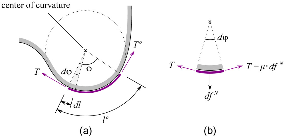
is a factor of nonintended curvature caused by construction errors (CEN 2010), which also exists when the cable is straight (

κ = 0

). As shown in Fig. 18(b), the normal force

d f^{N}

should be directed away from the center of curvature in order for the cable and the housing to be always in contact. In Eq. (31), the cable is assumed to be always in contact with the housing duct; in other words, the normal force

d f^{N}

is always positive at all points of the curve, and thus friction forces are acting along the whole length of the cable (Konyukhov and Shala 2021) [Figs. 18(a and b)]

d f^{N} = - κ T = - \frac{d φ}{d l} T > 0

(33)

When the condition in Eq. (33) is not satisfied, the cable and the housing are not in contact, and thus separation occurs. Separation does not occur if and only if the following conditions are satisfied: (1) the cable placement follows a convex function (e.g., parabolic) where the angle

φ

is a strictly monotonic function, and thus

sgn (κ) = sgn (d φ / d l)

is unchanging, or (2) the application of tension (i.e., actuation force) and the anchoring condition are oriented as the tangents at the cable extremities. Although several nonconvex functions (e.g., cosine and upside-down Gaussian) are employed in this work, separation is neglected by omitting the sign from

κ = d φ / d l

.

This way the effect of friction is estimated conservatively. For the sake of consistency with Eq. (29), the tension loss factor

γ

due to friction at the

i

th integration point is computed through a cumulative sum of the friction effect as follows:

γ_{i} = \exp {- μ ϖ l_{h} - μ \sum_{k = 1}^{i} Δ φ_{k}}; h = ⌈ \frac{i}{2} ⌉; \forall i = 1, \dots, 2 n^{seg}

(34)

where

Δ φ_{k}

,

\forall k = {1, \dots, i}

= angle formed by two neighboring unit tangent vectors

v_{k - 1}

and

v_{k}

Δ φ_{k} = \cos^{- 1} (\frac{v_{k}^{T} v_{k - 1}}{∥ v_{k} ∥ ∥ v_{k - 1} ∥})

(35)

Data Availability Statement

Some or all data, models, or code that support the findings of this study are available from the corresponding author upon reasonable request.

Acknowledgments

This work has been carried out within the framework of the Collaborative Research Centre 1244 “Adaptive Skins and Structures for the Built Environment of Tomorrow” under Grant No. 279064222. The authors gratefully acknowledge the German Research Foundation [Deutsche Forschungsgemeinschaft (DFG)] for providing core funding and their generous support. The authors thank Daniel Schmeer of Werner Sobek for his contribution to the benchmark against the voided slab configuration.

References

ACI (American Concrete Institute) Committee. 2015. Guide for the design and construction of structural concrete reinforced with fiber-reinforced polymer (FRP) bars. ACI 440.1R-15. Farmington Hills, MI: ACI.

Google Scholar

Afonso, S. B., F. Belblidia, E. Hinton, and G. R. Antonino. 2000. “A combined structural topology and sizing optimization procedure for optimum plates design.” In European congress on computational methods in applied sciences and engineering (ECCOMAS). Barcelona: ECCOMAS.

Google Scholar

Andrew, R. M. 2019. “Global

{CO}_{2}

emissions from cement production, 1928–2018.” Earth Syst. Sci. Data 11 (4): 1675–1710. https://doi.org/10.5194/essd-11-1675-2019.

Google Scholar

Berger, T., P. Prasser, and H. G. Rinke. 2013. “Einsparung von Grauer Energie bei Hochhaeusern.” Beton Stahlbetonbau 108 (6): 395–403. https://doi.org/10.1002/best.201300019.

Google Scholar

Blandini, L., W. Haase, S. Weidner, M. Böhm, T. Burghardt, D. Roth, O. Sawodny, and W. Sobek. 2022. “D1244: Design and construction of the first adaptive high-rise experimental building.” Front. Built Environ. 8 (Jun): 814911. https://doi.org/10.3389/fbuil.2022.814911.

Google Scholar

Brent, R. P. 1973. “Chapter 4: An algorithm with guaranteed convergence for finding a zero of a function.” In Algorithms for minimization without derivatives. Englewood Cliffs: Prentice-Hall.

Google Scholar

Campbell, T. I., and L. Chitnuyanondh. 1975. “Horizontally-curved continuous post-tensioned concrete beams.” PCI J. 20 (2): 58–71. https://doi.org/10.15554/pcij.03011975.58.71.

Google Scholar

CEN (European Committee for Standardization). 2002. Basis of structural design. EN 1990 Eurocode. Brussels, Belgium: CEN.

Google Scholar

CEN (European Committee for Standardization). 2010. Design of concrete structures. EN 1992 Eurocode 2. Brussels, Belgium: CEN.

Google Scholar

Energie Baden-Württemberg. 2022. “EnBW environmental data 2022.” Accessed June 5, 2023. https://www.enbw.com/media/konzern/docs/umweltschutz/umweltdatentabelle_enbw_2022_enbw-com.xlsx.

Google Scholar

ENERPAC. 2016. “E328e Industrial Tools—Europe.” Accessed May 4, 2023. https://www.enerpac.com/enus/.

Google Scholar

European Commission. 2016. Study on the energy saving potential of increasing resource efficiency. Brussels, Belgium: European Commission, Directorate-General for Environment.

Google Scholar

European Environment Agency. 2022. Trends and projections in Europe 2022. Copenhagen, Denmark: European Environment Agency.

Google Scholar

Fanella, D. A., M. Mahamid, and M. Mota. 2017. “Flat plate–voided concrete slab systems: Design, serviceability, fire resistance, and construction.” Pract. Period. Struct. Des. Constr. 22 (3): 04017004. https://doi.org/10.1061/(ASCE)SC.1943-5576.0000322.

Google Scholar

Felippa, C. A. 2004. Introduction to finite element methods. Boulder, CO: Univ. of Colorado.

Google Scholar

Geuzaine, C., and J. F. Remacle. 2009. “Gmsh: A 3-D finite element mesh generator with built-in pre- and post-processing facilities.” Int. J. Numer. Methods Eng. 79 (11): 1309–1331. https://doi.org/10.1002/nme.2579.

Google Scholar

Halpern, A. B., D. P. Billington, and S. Adriaenssens. 2013. “The ribbed floor slab systems of pier Luigi Nervi.” In Proc., Int. Association for Shell and Spatial Structures (IASS) Symp. 2013. Madrid, Spain: International Association for Shell and Spatial Structures.

Google Scholar

Huberman, N., D. Pearlmutter, E. Gal, and I. A. Meir. 2015. “Optimizing structural roof form for life-cycle energy efficiency.” Energy Build. 104 (Oct): 336–349. https://doi.org/10.1016/j.enbuild.2015.07.008.

Google Scholar

Iori, T. 2012. “Le plancher à nervures isostatiques de Nervi.” In L’architrave, le plancher, la plate-forme: Nouvell histoire de la construction, edited by R. Gargiani, 755–760. Lausanne, Switzerland: Presses Polytechniques et Universitaires Romandes.

Google Scholar

Johansen, K. W. 1962. Yield-line theory. Washington, DC: Cement and Concrete Association.

Google Scholar

Johnson, K. L. 1985. Contact mechanics. Cambridge, UK: Cambridge University Press.

Crossref

Google Scholar

Jones, E., T. Oliphant, and P. Peterson. 2001. “SciPy: Open source scientific tools for Python.” Accessed June 8, 2023. https://www.scipy.org.

Google Scholar

Kelleter, C., T. Burghardt, H. Binz, L. Blandini, and W. Sobek. 2020. “Adaptive concrete beams equipped with integrated fluidic actuators.” Front. Built Environ. 6 (Jul): 91. https://doi.org/10.3389/fbuil.2020.00091.

Google Scholar

Khosravi, P., R. Sedaghati, and R. Ganesan. 2007. “Optimization of stiffened panels considering geometric nonlinearity.” J. Mech. Mater. Struct. 2 (7): 1249–1265. https://doi.org/10.2140/jomms.2007.2.1249.

Google Scholar

Konyukhov, A., and S. Shala. 2021. “New benchmark problems for verification of the curve-to-surface contact algorithm based on the generalized Euler-Eytelwein problem.” Int. J. Numer. Methods Eng. 123 (2): 411–443. https://doi.org/10.1002/nme.6861.

Google Scholar

Lam, Y. C., and S. Santhikumar. 2003. “Automated rib location and optimization for plate structures.” Struct. Multidiscip. Optim. 25 (1): 35–45. https://doi.org/10.1007/s00158-002-0270-7.

Google Scholar

Li, L., C. Liu, W. Zhang, Z. Du, and X. Guo. 2021. “Combined model-based topology optimization of stiffened plate structures via MMC approach.” Int. J. Mech. Sci. 208 (Oct): 106682. https://doi.org/10.1016/j.ijmecsci.2021.106682.

Google Scholar

Ministry for Housing, Urban Development and Building, Federal Republic of Germany. 2013. “ÖKOBAUDAT—Sustainable Construction Information Portal.” Accessed June 5, 2023. https://www.oekobaudat.de.

Google Scholar

Nervi, P. L. 1956. Structures. New York: F.W. Dodge Corp.

Google Scholar

Neuhäuser, S. 2014. “Untersuchungen zur Homogenisierung von Spannungsfeldern bei adaptiven Schalentragwerken mittels Auflagerverschiebung.” Doctoral dissertation, Institute for Lightweight Structures and Conceptual Design (ILEK), Univ. of Stuttgart.

Google Scholar

Nigl, D., O. Gericke, L. Blandini, and W. Sobek. 2022. “Numerical investigations on the biaxial load-bearing behaviour of graded concrete slabs.” In Proc., Fib Int. Congress. Lausanne, Switzerland: International Federation for Structural Concrete (fib).

Google Scholar

Nitzlader, M., M. J. Bosch, H. Binz, M. Kreimeyer, and L. Blandini. 2022a. “Actuation of concrete slabs under bending with integrated fluidic actuators.” In Proc., World Congress on Computational Mechanics. Barcelona, Spain: International Association for Computational Mechanics.

Google Scholar

Nitzlader, M., S. Steffen, M. J. Bosch, H. Binz, M. Kreimeyer, and L. Blandini. 2022b. “Designing actuation concepts for adaptive slabs with integrated fluidic actuators using influence matrices.” Civ. Eng. 3 (3): 809–830. https://doi.org/10.3390/civileng3030047.

Google Scholar

OECD. 2019. Global material resources outlook to 2060: Economic drivers and environmental consequences. Paris: OECD Publishing.

Crossref

Google Scholar

Olivier, J. G. J., K. M. Schure, and J. A. H. W. Peters. 2017. Trends in global ${CO}_{2}$ and total greenhouse gas emissions. The Hague, Netherlands: PBL Netherlands Environmental Assessment Agency.

Google Scholar

Pacheco, P., and A. Adao da Fonseca. 2002. “Organic prestressing.” J. Struct. Eng. 128 (3): 400–405. https://doi.org/10.1061/(ASCE)0733-9445(2002)128:3(400).

Google Scholar

Ranaudo, F., T. Van Mele, and P. Block. 2021. “A low-carbon, funicular concrete floor system: Design and engineering of the HiLo floors.” In Proc., IABSE Congress, Ghent 2021: Structural Engineering for Future Societal Needs. Zurich, Switzerland: International Association for Bridge and Structural Engineering.

Google Scholar

Reinhorn, A. M., T. T. Riley, M. A. Soong, and R. C. Lin. 1993. “Full-scale implementation of active control. II: Installation and performance.” J. Struct. Eng. 119 (6): 1935–1960. https://doi.org/10.1061/(ASCE)0733-9445(1993)119:6(1935).

Google Scholar

Reksowardojo, A. P., G. Senatore, A. Srivastava, C. Carrol, and I. F. C. Smith. 2022. “Design and testing of a low-energy and -carbon prototype structure that adapts to loading through shape morphing.” Int. J. Solids Struct. 252 (Oct): 111629. https://doi.org/10.1016/j.ijsolstr.2022.111629.

Google Scholar

Remacle, J.-F., F. Henrotte, T. Carrier-Baudouin, E. Bêchet, E. Marchandise, C. Geuzaine, and T. Mouton. 2010. “A frontal Delaunay quad mesh generator using the L∞ norm.” Int. J. Numer. Methods Eng. 94 (5): 455–472. https://doi.org/10.1002/nme.4458.

Google Scholar

Rippmann, M., A. Liew, V. Mele, and P. Block. 2018. “Design, fabrication and testing of discrete 3D sand-printed floor prototypes.” Mater. Today Commun. 15 (Jun): 254–259. https://doi.org/10.1016/j.mtcomm.2018.03.005.

Google Scholar

Schmeer, D. 2021. Mesogradierung von Betonbauteilen: Herstellung und Tragverhalten von Betonbauteilen mit integrierten mineralischen Hohlkugeln. Düren, Germany: Shaker.

Google Scholar

Schmeer, D., and W. Sobek. 2018. “Gradientenbeton.” In Vol. 108 of Beton Kalender 2019: Parkbauten Geotechnik und Eurocode 7, 455–476. Berlin: Ernst & Sohn.

Crossref

Google Scholar

Schnellenbach-Held, M., A. Fakhouri, D. Steiner, and O. Kühn. 2013. “Upgrade of concrete bridges by adaptive prestressing.” In Proc., IABSE Conf.: Assessment, Upgrading and Refurbishment of Infrastructures. Zurich, Switzerland: The International Association for Bridge and Structural Engineering.

Google Scholar

Schnellenbach-Held, M., and D. Steiner. 2014. “Self-tuning closed-loop fuzzy logic control algorithm for adaptive prestressed structures.” Struct. Eng. Int. 24 (2): 163–172. https://doi.org/10.2749/101686614X13830790993528.

Google Scholar

Senatore, G., P. Duffour, S. Hanna, F. Labbe, and P. Winslow. 2011. “Adaptive structures for whole-life energy savings.” J. Int. Assoc. Shell Spatial Struct. 52 (4): 233–240.

Google Scholar

Senatore, G., P. Duffour, and P. Winslow. 2019. “Synthesis of minimum energy adaptive structures.” Struct. Multidiscip. Optim. 60 (3): 849–877. https://doi.org/10.1007/s00158-019-02224-8.

Google Scholar

Senatore, G., P. Duffour, P. Winslow, and C. Wise. 2018. “Shape control and whole-life energy assessment of an ‘infinitely stiff’ prototype adaptive structure.” Smart Mater. Struct. 27 (1): 015022. https://doi.org/10.1088/1361-665X/aa8cb8.

Google Scholar

Senatore, G., and A. P. Reksowardojo. 2020. “Force and shape control strategies for minimum energy adaptive structures.” Front. Built Environ. 6 (Jul): 105. https://doi.org/10.3389/fbuil.2020.00105.

Google Scholar

Simulia. 2009. “ABAQUS version 6.6 documentation.” Accessed July 6, 2023. https://classes.engineering.wustl.edu/2009/spring/mase5513/abaqus/docs/v6.6/books/usb/default.htm?startat=pt06ch23s06alm15.html.

Google Scholar

Soong, T. 1988. “Active structural control in civil engineering.” Eng. Struct. 10 (2): 74–84. https://doi.org/10.1016/0141-0296(88)90033-8.

Google Scholar

USGS. 2016. “U.S. Geological Survey: Mineral commodity summaries 2016.” Accessed June 8, 2023. http://minerals.usgs.gov/minerals/pubs/com-modity/cement/.

Google Scholar

Wang, Y., and G. Senatore. 2020. “Minimum energy adaptive structures—All-in-one problem formulation.” Comput. Struct. 236 (Aug): 106266. https://doi.org/10.1016/j.compstruc.2020.106266.

Google Scholar

Weidner, S., et al. 2018. “The implementation of adaptive elements into an experimental high-rise building.” Steel Constr. Des. Res. 11 (2): 109–117. https://doi.org/10.1002/stco.201810019.

Google Scholar

Wu, H., A. Liew, T. Van Mele, and P. Block. 2020. “Analysis and optimisation of a rib-stiffened vaulted floor for dynamic performance.” Eng. Struct. 213 (Jun): 110577. https://doi.org/10.1016/j.engstruct.2020.110577.

Google Scholar

Information & Authors

Information

Published In

Journal of Structural Engineering

Volume 150 • Issue 1 • January 2024

Copyright

This work is made available under the terms of the Creative Commons Attribution 4.0 International license, https://creativecommons.org/licenses/by/4.0/.

History

Received: Dec 19, 2022

Accepted: Aug 15, 2023

Published online: Oct 28, 2023

Published in print: Jan 1, 2024

Discussion open until: Mar 28, 2024

Authors

Affiliations

Arka P. Reksowardojo, Ph.D., A.M.ASCE https://orcid.org/0000-0002-5626-430X

Scientist, Institute for Lightweight Structures and Conceptual Design (ILEK), Univ. of Stuttgart, Stuttgart 70569, Germany. ORCID: https://orcid.org/0000-0002-5626-430X

View all articles by this author

Gennaro Senatore, Ph.D. https://orcid.org/0000-0001-7418-9713 [email protected]

Research Group Leader (Senior Scientist), Institute for Lightweight Structures and Conceptual Design (ILEK), Univ. of Stuttgart, Stuttgart 70569, Germany (corresponding author). ORCID: https://orcid.org/0000-0001-7418-9713. Email: [email protected]

View all articles by this author

Manfred Bischoff, Dr.Ing. https://orcid.org/0000-0003-1538-4281

Professor, Institute for Structural Mechanics (IBB), Univ. of Stuttgart, Stuttgart 70569, Germany. ORCID: https://orcid.org/0000-0003-1538-4281

View all articles by this author

Lucio Blandini, Dr.Ing. https://orcid.org/0000-0002-4592-6347

Professor, Institute for Lightweight Structures and Conceptual Design (ILEK), Univ. of Stuttgart, Stuttgart 70569 Germany. ORCID: https://orcid.org/0000-0002-4592-6347

View all articles by this author

Metrics & Citations

Metrics

Citations

Download citation

If you have the appropriate software installed, you can download article citation data to the citation manager of your choice. Simply select your manager software from the list below and click Download.

Abstract

Introduction

Previous Work

New Contribution

Active Rib

Design Method

Control Strategy

Controller Design

Adaptive Tensioning System

Case Study

Benchmarking with Respect to Cable Profiles

Benchmarking with Respect to Active Rib Layouts

Deflection and Stress Behavior

Mass and Energy Assessment

Equivalent Carbon Assessment

Discussion

Conclusion

Appendix I. Equivalent Forces from a Curvilinear Cable under Tension

Cable Strain and Nodal Displacements Relationship

Equivalent Forces through the Principle of Virtual Work

Appendix II. Tensile Loss as a Result of Friction

Data Availability Statement

Acknowledgments

References

Information

Published In

Copyright

History

Authors

Affiliations

Metrics

Citations

Download citation

Figures

Other

Share

Copy the content Link

Share with email

Share

Request Username

Create a new account

Change Password

Password Changed Successfully

Verify Phone

Congrats!