Numerical Optimization of Wastewater Treatment Plant Design for a High-Nitrate Industrial Waste
Publication: Journal of Environmental Engineering
Volume 149, Issue 12
Abstract
This study develops an optimal design of a municipal water resource recovery facility (WRRF) to treat a high-nitrate industrial waste. The study demonstrated two basic results: first, that a numerical optimization scheme has the potential to significantly reduce construction and operating costs for wastewater treatment. Second, it demonstrated the potential for high-nitrate industrial waste to partially satisfy the electron acceptor requirement for treating municipal wastewater, whereas the wastewater reduces the demand for supplemental carbon for treating the nitrate. The optimization scheme sought to minimize an objective function, which included annualized construction costs, operating costs, and penalties for environmental performance. The optimization algorithm used was the Nelder–Mead method. This was coupled with a commercial activated sludge simulation program in an iterative calculation to predict the performance of successive process designs. The optimized process had a predicted 89% removal of total nitrogen from the combined municipal and industrial wastewater. The optimization reduced the objective function by 53% in comparison to initial designs that were manually optimized without the algorithm. The supplemental carbon requirement was reduced by 15.5% over literature values. The unique aspect of this research is the coupling of an external biological simulation model with a numerical optimization algorithm that could significantly improve the cost-effectiveness of process design along with operating costs and effluent quality. Furthermore, it demonstrates the feasibility of treating these types of wastes in a municipal facility.
Practical Applications
The results of this study indicate that coupling a numerical optimization scheme with commercial activated sludge (or other) process simulation models has the potential to make the construction and operation of treatment facilities significantly more cost effective. This study also shows that high-nitrate industrial wastewater has the potential to be treated in combination with municipal wastewater, reducing the cost of supplemental carbon for the nitrate reduction while simultaneously reducing the cost of aeration for the wastewater treatment. We began by developing a daily cost of treatment (the objective function) based on the annualized cost for design parameters such as aeration tank and clarifier size plus operating costs for aeration and pumping energy, methanol dosage, and solids disposal. Added to this were cost penalties for effluent discharge of biochemical oxygen demand (BOD), total suspended solids (TSS), and nitrogen species. The optimization scheme iteratively makes adjustments to the design parameters to seek to minimize the total costs in the objective function. The development of an objective function that includes capital and operating costs and environmental performance factors is unique to this study.
Introduction
Many industries produce waste with very high nitrate concentrations, typically greater than as nitrogen. Discharge of these nitrate-containing wastes can create serious environmental and public health problems. These problems include eutrophication and its resultant effect on water quality and ecology and migration of nitrate to surface water and groundwater, impacting the safety of drinking water sources (USEPA 2022b; Dubrovsky et al. 2010). Successfully treating and disposing of this waste can be expensive and problematic because there has been an increase in environmental regulations governing nitrogen discharges (USEPA 2015, 2022a). The most common way to remove nitrate from wastewater is through the biological process of denitrification (Metcalf and Eddy 2014).
Biological denitrification is well understood and widely used for nitrogen removal from municipal wastewater (Barnard 2006). Biological denitrification is a heterotrophic process. In the absence of oxygen, heterotrophic organisms use either nitrite or nitrate as the electron acceptor rather than oxygen. However, applying it to high-nitrate industrial wastes discharged to an existing water resource recovery facility (WRRF) can be difficult because of design constraints at the facility, the risk of not meeting low effluent total nitrogen (TN) permit limits, or the concern that some of the chemical constituents in the industrial waste might be inhibitory or toxic to the microorganisms.
There have been several studies evaluating different biological methods of reducing nitrate from various sources with different nitrate concentrations. Some of the studies used specially cultured microorganisms. For example, Fernández-Nava et al. (2008) studied denitrification of stainless-steel production wastewater with a concentration between 600 and using a specialized microbial community isolated from either landfill leachate or wastewater solids. Cyplik et al. (2012) studied biological treatment of wastewater from explosive production with a concentration of using an engineered microbial population isolated from petroleum-contaminated soil. Dhamole et al. (2007) studied the effect of using bacteria isolated from a fertilizer plant sludge to reduce a synthetic waste with a concentration of . One study evaluated an anoxic-oxic membrane bioreactor (MBR) process (Shen et al. 2009), and others evaluated various external carbon sources and carbon-to-nitrogen ratios (Fernández-Nava et al. 2008; Mohan et al. 2016; DeFilippis et al. 2013). Glass and Silverstein (1999) studied the removal of nitrate from a waste containing and a very high salinity using typical activated sludge bacteria. There was no research identified that studied discharging these waste products to a municipal wastewater treatment facility. If the industrial waste is discharged to a municipal system, the organic carbon in the wastewater could reduce the nitrate, thus reducing the expense of carbon supplementation, whereas the nitrate oxidizes the biochemical oxygen demand (BOD) in the waste, potentially reducing aeration costs.
The goal of this study is to evaluate the concept of discharging this waste directly to a typical municipal wastewater treatment facility to determine any design modifications necessary to the facility, to optimize the design using a numerical optimization algorithm, and to demonstrate a financial benefit to the municipality through energy or other cost savings by using the carbon in the wastewater to reduce the demand for supplemental carbon. This is based on the “circular economy” concept wherein the waste produced by one activity becomes a resource for another (USEPA 2009). In this case, the circularity works in both directions–the industrial nitrate waste is used to oxidize the wastewater, reducing the energy requirement for aeration, and the wastewater chemical oxygen demand (COD) is used to reduce the nitrate waste, potentially reducing the need for supplemental carbon.
Our approach consisted of the following steps:
•
An objective function (OF) was defined that encompassed all the relevant costs for the process, including capital costs, operating costs, and penalties to account for process performance.
•
Initial design configurations were developed by a manual suboptimization approach using BioWin process simulation software (EnviroSim).
•
The Nelder–Mead simplex optimization algorithm was used to refine the design parameters for the best configuration from the previous step.
A next step (currently underway) is experimental validation of the optimized design using a pilot plant.
Wastewater Characteristics
The flow rate of the domestic wastewater was assumed to be (10.5 MGD), and the flow rate for the industrial waste was (2.5 MGD). The influent wastewater and industrial waste characteristics for this study are shown in Table 1.
| Parameter | Municipal wastewater | Industrial waste | Combined influent |
|---|---|---|---|
| , | 39,750 | 9,464 | 49,210 |
| COD, | 537 | 14 | 436 |
| TKN, | 47 | — | 38 |
| , | 33 | — | 27 |
| , | 0 | 384 | 74 |
| , | 0 | 6 | 1 |
Process Design and Model Simulations
Before beginning the optimization procedure, an initial process configuration and design parameters needed to be established. The approach used here is a conventional design methodology coupled with numerical process simulation. Three process configurations were considered. The first was the modified Ludzack–Ettinger (MLE) nitrification–denitrification process. For a second configuration, the MLE itself was modified to incorporate a step-feed of the industrial nitrate waste in order to distribute the denitrification rate through the reactor. The third configuration was an attempt to increase the biologically available COD by incorporating a sidestream fermentation reactor.
The denitrification reaction shown in Eq. (1) (neglecting cell yield) is based on using methanol as the electron donor/carbon source (Metcalf and Eddy 2014)
(1)
If there is insufficient carbon in the wastewater, an external source of carbon is added, typically methanol or glycerol (Metcalf and Eddy 2014). From Eq. (1), the stoichiometric requirement for methanol is . The stoichiometric oxygen demand of methanol is . Thus, the stoichiometric carbon-to-nitrogen ratio (), with carbon expressed as COD, is (when not considering biomass yield). In practice, ratios about twice this value are used to ensure complete denitrification (Metcalf and Eddy 2014).
The preliminary process designs were validated using computer process models. Mathematical modeling of biological nitrogen removal processes has been used successfully for many years for evaluation, design, and process control (Daigger and Nolasco 1995; Daigger 2011). There are various proprietary modeling software packages available. Even though they have different interfaces and outputs, they are all based on the IWA ASM models (Henze et al. 2006). BioWin process simulation software (EnviroSim) was used for this project. It is a commercial software program that allows for the numerical simulation of various physical and chemical processes used in wastewater treatment. It is used throughout the sector for designing and upgrading wastewater processes and is based on the IWA ASM3 models. The default model parameters in the BioWin software were used in this study.
Numerical Optimization
Any process has numerous parameter choices that must be made. Numerical optimization is a procedure for selecting a combination of parameters that minimizes (or maximizes) a function, called the objective function (OF), that expresses the goal of the design. By incorporating design and operating costs as well as penalties for effluent quality, optimization of wastewater process design can ensure that a WRRF meets permit requirements at the lowest operating and capital costs possible. The OF can express the trade-offs in process design. For example, methanol costs for denitrification can be significant, but reducing methanol dosage may result in increasing costs associated with discharging nitrate with the effluent. By expressing each of the objectives associated with a design one in terms of cost, one can express the multiple-objective problem as having a single objective. Wastewater treatment design is a nonlinear problem with multiple variables, so optimizing design is a complex problem requiring an iterative method. It is important that the objective function include all relevant variables that could affect treatment costs. Omission of an important variable could drive the optimization to sacrifice that factor. For example, if a factor were not included for solids disposal cost, then the algorithm would tend to drive the process toward having a lower solids retention time (SRT), resulting in a higher solids disposal cost.
Numeric optimization algorithms have been used for various wastewater engineering problems. Rafati et al. (2022) studied the use of the particle swarm optimization algorithm coupled with the activated sludge model to determine the optimum rate of return activated sludge, internal recycle, and value of the oxygen transfer coefficient. Chen et al. (2020) examined the use of a multiobjective function for optimizing design. Zhang et al. (2014) evaluated the use of multiobjective optimization for optimizing effluent quality and operating cost, and Dai et al. (2016) evaluated the use of multiobjective optimization coupled with the activated sludge model to optimize effluent quality, operation cost, and operation stability. Chen et al. (2014) studied the use of the multiobjective optimization for optimizing performance and energy consumption. Ludwig et al. (2011) used a genetic algorithm coupled with the GPX-S wastewater simulation software to optimize relaxation and filtration times of submerged microfiltration flat modules in membrane bioreactors. Khoja et al. (2018) used a particle swarm optimization algorithm as a method for the identification of parameters for modeling the activated sludge process for control but not design. Hakanen et al. (2013) combined the GPX-S wastewater simulation software with multiobjective optimization software for optimizing wastewater design and operation. Their approach required involvement of a “decision-maker” to make trade-off decisions for conflicting objectives. Alvarez-Vázquez et al. (2002) compared the use of three different numerical algorithms: an interior point algorithm, the Nelder and Mead (1965) simplex method, and a duality method for optimizing the location of wastewater outfalls, concluding that the Nelder–Mead algorithm provided the best results. Kim et al. (2015) successfully used the Nelder–Mead algorithm for optimizing wastewater treatment to minimize greenhouse gas emission. The current study is novel in its coupling of a biological simulation model with a numerical algorithm to optimize a combination of design (capital) costs, performance (permit compliance), and operating costs.
Objective Function
A critical step in optimization is developing the objective function (OF). The OF should express all major capital and operating costs, plus penalties based on effluent quality. Omitting a factor that realistically should be included may result in unrealistic, or at least uneconomic, values for that factor.
The objective function in this work had two factors for capital costs, four factors for operating costs, and four factors for effluent quality. Table 2 lists each cost component () of the OF, which when multiplied by its corresponding cost factor () yields the contribution of that component to the OF in dollars per day. These are then summed to yield the total OF
(2)
| Cost component | Cost factor | Units | Reference |
|---|---|---|---|
| Capital costs | |||
| Reactor | 0.216 | (Fournier, personal communication, 2022) | |
| Clarifier | 0.003175 | (Fournier, personal communication, 2022) | |
| Operating costs | |||
| MeOH | 338 | (Mamaroneck WPCA, personal communication, 2021) | |
| Internal recycle | 544 | () | (Metcalf and Eddy 2014; EIA 2021) |
| Aeration cost | 0.036 | (EIA 2021) | |
| Solids disposal | 0.529 | (NYC 2021) | |
| Effluent quality | |||
| BOD + TSS | 0.162 | (USEPA 2022c) | |
| TKN | 10.85 | (CTNCAB 2021) | |
| Nitrate | 2.82 | (CTNCAB 2021) | |
| Nitrite | 2.23 | (CTNCAB 2021) | |
The actual values of the cost factors in Table 2 could be different for individual cases. This would change the resulting optimum design. However, this would not be expected to affect the validity of the design procedure that is being developed here.
Capital costs were amortized so that both capital and operating costs could be expressed in units of dollars per day. The capital cost factors include the costs for reactor volume and clarifier capacity. The reactor costs were calculated based on current construction cost amortized over 20 years at 3.0% interest. The reactor cost is based on the total volume of all reactors, whether aerobic, anoxic, or anaerobic. Reactor cost was $4.50M per million gallons of reactor volume. This value was developed using 2019 construction costs in Connecticut (Fournier, personal communication, 2022). The clarifier cost was based on the solids loading rate, which effectively drives the size of the unit and the current construction cost using 2019 construction costs in Connecticut (Fournier, personal communication, 2022).
The operating cost factors include the cost of electricity for aeration (EIA 2021), electrical cost for internal recycle pumping based on the power requirement (Metcalf and Eddy 2014; EIA 2021), the cost of methanol (Mamaroneck WPCA, personal communication, 2021), and the disposal cost for waste activated sludge (NYC 2021).
The effluent quality cost factors are penalties based on what it would cost either for permit violations or additional treatment costs. These included factors for BOD and total suspended solids (TSS) combined and for the different forms of effluent nitrogen. The BOD+TSS cost factor was based on the cost of permit violations for BOD and TSS (USEPA). The nitrogen cost factors were based on the Connecticut Nitrogen Trading program (CTNCAB 2021) cost per pound of TN discharged and other nitrogen-related costs for removal of TKN, nitrate, and nitrite.
Nelder–Mead Optimization Algorithm
The Nelder–Mead algorithm (Nelder and Mead 1965) was chosen for the optimization of the proposed design because it is robust with respect to complex process response surfaces, yet it is efficient in terms of computational iterations required and does not require computation of derivatives. The Nelder–Mead optimization algorithm was implemented using a program implemented in the MATLAB programming and numeric software package (MathWorks 2008). The program is provided in the Appendix, “Nelder Mead Code.” It is useful for multidimensional, unconstrained optimization without derivatives (Scholarpedia 2009). A major advantage is that it tends to require many fewer function evaluations (simulations in this context) than other methods. The algorithm uses the following steps (Scholarpedia 2009):
1.
An initial simplex is generated. The simplex is a set of unique points in an space, where is the number of input variables. In two dimensions, the simplex is a triangle; in three, it is a tetrahedron. The initial simplex is designed to encompass the range of expected input values such that the optimum combination is within or near the simplex. The procedure used to develop the initial simplex in this study is described subsequently.
2.
Transformation of the simplex. A new simplex is computed to replace the current one and then replace the worst vertex with better points by one of the following transformations: reflection, expansion, contraction, or shrinking. Essentially, this is a new set of input variables proposed by the Nelder–Mead algorithm.
3.
A new objective function value is computed and input to the algorithm. Step 2 is repeated until the simplex converges on the optimum to within some convergence criterion.
Optimization Procedure
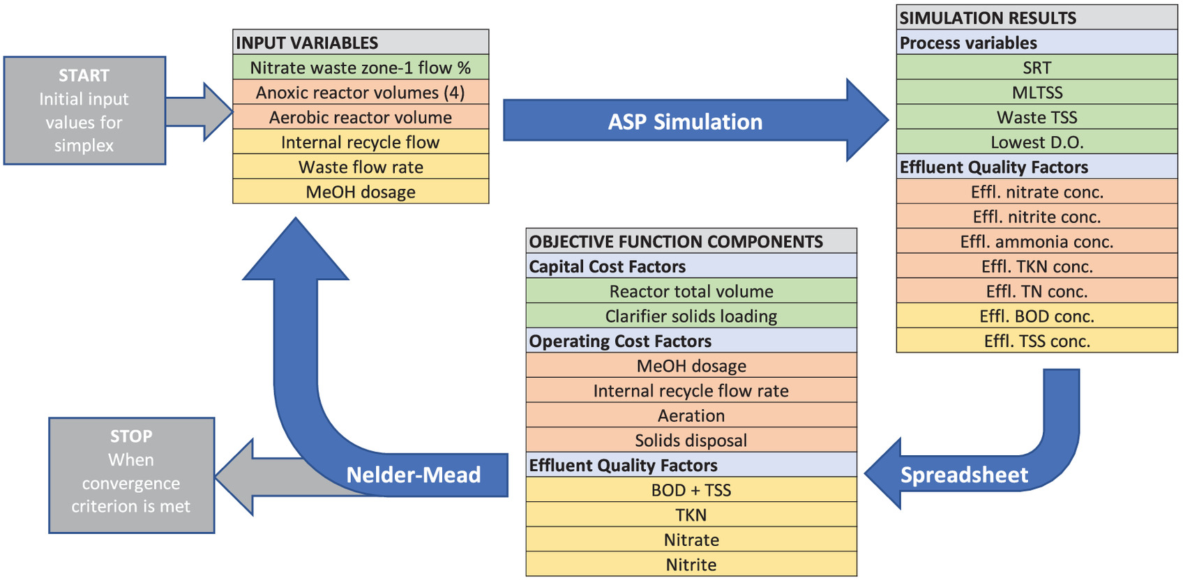
The numerical optimization procedure consisted of the following iterative steps combining the use of process simulation, objective function calculation, and Nelder–Mead algorithm. Fig. 1 graphically illustrates the procedure described by these steps.
1.
A set of input variables is defined consisting of the design and operating parameters required to simulate the process. In this study, . Fig. 1 shows the nine input variables used in this study.
2.
An initial set of maximum and minimum values is selected for each of the input variables that are judged to span the feasible range of each. These values define opposite corners of an hypercube. The starting simplex for the Nelder–Mead algorithm will consist of all the vertices of the hypercube adjacent to the vertex consisting of all minimum values. Each vertex of the simplex is a unique combination of input values.
3.
For each set of input variables (corresponding to one of the vertices), a simulation is run using BioWin. BioWin computes the process performance, which is summarized as the set of simulation results, as listed in Fig. 1.
4.
5.
The resulting OF value is entered into the Nelder–Mead program. The program checks to see if convergence was attained. If it was, the procedure is stopped.
6.
If the convergence criterion is not reached, the next iteration is begun with Step 3.
Before beginning the use of the numerical optimization procedure, a preliminary investigation was conducted using BioWin simulation alone. The preliminary investigation tested four treatment configurations. The best among these was selected for optimization.
The selected configuration had nine independent design and operating input variables (Fig. 1). The output from the simulation included the simulation results, as shown in Fig. 1. The values for the input variables and simulation results were entered into a spreadsheet to compute the OF using the cost factors from Table 2.
If an output variable was not realistic (for example, if the waste activated sludge flow rate was zero, or if there was a negative value for any of the variables) the objective function was doubled, and that value was entered into the next iteration of the Nelder–Mead algorithm.
The convergence criterion was chosen so that iterations were stopped when the difference between the largest and smallest OF values associated with any of the simplex vertices was less than $500 per day. The steps of the procedure as shown in Fig. 1 were performed by manually copying data between the three software programs (BioWin, Excel, and the MATLAB Nelder–Mead program). The potential exists for this manual procedure to be automated within a biological simulation program.
Results
The goal of the initial simulations was to determine which preliminary process would yield the highest nitrate removal at lowest cost. Cost was reflected by the value of OF for the configuration and operating conditions. As mentioned, four basic process configurations were studied before settling on one configuration to use in the complete optimization study. Effluent TN was used as the criterion for selecting which preliminary process would be used in the optimization part of the study.
MLE Process
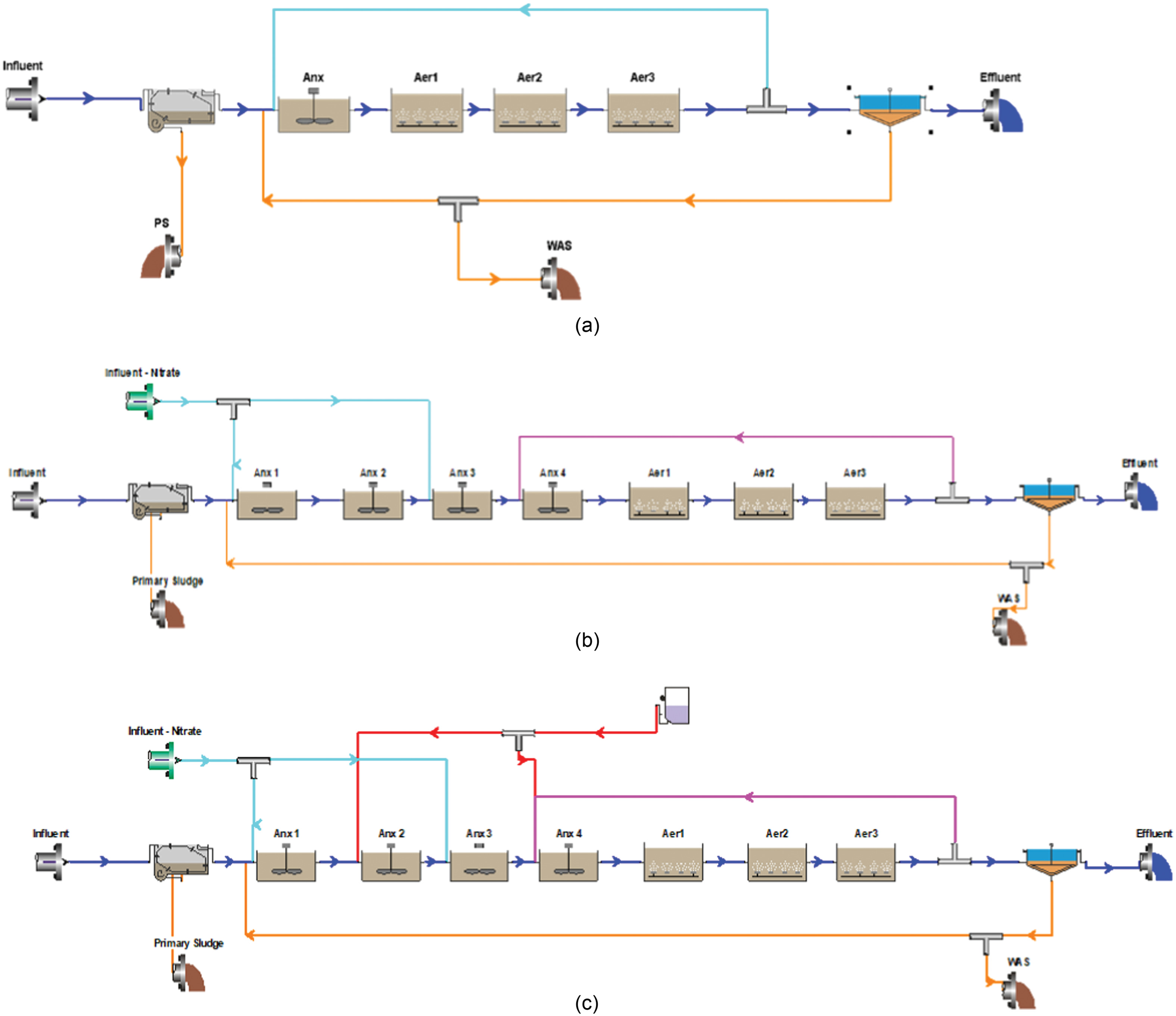
A common design used for biological nitrogen removal is the modified Ludzack–Ettinger process, which has a preanoxic zone followed by an aerobic zone [Fig. 2(a)]. In the MLE process, ammonia is oxidized to nitrate in the aerobic zone (nitrification), and the nitrate is then recycled to the anoxic zone for denitrification using a high-volume mixed liquor recycle. The MLE process does use not typically use an external carbon source but only the carbon available from the wastewater.
For an MLE process for domestic wastewater, the anoxic zone is typically about 25% to 30% of the total reactor volume (Metcalf and Eddy 2014). However, due to the high nitrate loading for this study, the anoxic volume needed to be considerably larger. This was achieved by varying the hydraulic residence time (HRT) of the anoxic reactor (). All HRT values in this work, except for the sidestream reactor described subsequently, are defined as the volume of the relevant reactors divided by the total flow through the process, in this case consisting of the influent wastewater plus the industrial waste.
The purpose of this series was to determine the quantity of nitrogen that could be removed without adding external sources of carbon. Therefore, the only carbon source for these simulations was the influent wastewater. The simulations evaluated the effects of chemical oxygen demand to total nitrogen () ratio and also anoxic hydraulic retention time (). For this series, the industrial waste was added at the headworks of the treatment facility and mixed with the influent wastewater. All simulations were performed at 20°C and a 10-day SRT and used the BioWin default kinetics. The results of the simulations would be different at other temperatures, but for the purpose of this study, a constant temperature of 20°C is adequate to demonstrate the concept. The optimization procedure developed here would not be affected by the choice of different parameters.
Although the stoichiometric ratio is 2.55, the typical ratio used for wastewater treatment facilities ranges from 4.0 to 5.0 because not all of the COD in wastewater is readily bioavailable (Metcalf and Eddy 2014). The influent wastewater characteristics used in these simulations (Table 1) resulted in a ratio of 2.6 when using primary treatment or 3.9 in the case of assuming that there is no primary treatment.
The value of varied from 2.0 to 14.2 h, whereas aerobic was maintained at a constant 6 h. The results of these simulations are shown in Table 3 and clearly show the relationship between ratio and effluent nitrogen at a given . Removal of TN increased with both ratio and . The lowest effluent TN concentration was , achieved with a ratio and an anoxic HRT of 14.2 h.
| HRT, h | %TN Rem | Eff TN | |
|---|---|---|---|
| 2.6 | 2 | 28 | 82 |
| 6.1 | 36 | 75 | |
| 10.2 | 41 | 69 | |
| 12.2 | 44 | 67 | |
| 14.2 | 43 | 64 | |
| 3.9 | 2 | 43 | 65 |
| 6.1 | 53 | 56 | |
| 10.2 | 61 | 47 | |
| 12.2 | 64 | 44 | |
| 14.2 | 65 | 42 |
Step-Nitrate Feed with and without Methanol Addition
The next series of simulations evaluated the effect of step-feeding the industrial waste at two locations within the reactor rather than discharging it directly to the headworks of the WRRF and varying the by dosing with methanol. The rationale for step-feeding was to try to equalize the quantity of COD available for the organisms in more than one zone. The process flow configuration used for this series is shown in Fig. 2(b).
The first set of simulations with this configuration evaluated nitrate removal without the addition of external carbon but divided the industrial waste discharge equally into two different zones: Anox 1 and Anox 3 [Fig. 2(b)]. The total anoxic HRT was 11.7 h, and the total aerobic HRT was 5.7 h. The TN mass entering the biological reactors was , and the mass leaving the system was , for a 44% removal. Another simulation used the same HRTs but added the industrial waste only in Anox 1. The removal rate did not change, showing that the addition point had little or no effect. Additionally, these simulations showed that without the addition of external carbon, it was not possible to get high removals of TN with this configuration. The best effluent TN concentration for step-feeding without methanol addition was .
For the next series of simulations, methanol was fed to the reactor [Fig. 2(c)] in various amounts ranging from 0.4 to , resulting in ratios from 2.9 to 5.1 based on the combined wastewater and methanol COD. The same reactor volumes and operating conditions were used in this series as in the previous series but with methanol dose being the only variable. The results are shown in Table 4. The highest percent removal, 93%, and the lowest effluent TN, , were achieved using a methanol dose of . The resulting operating cost for methanol to achieve this effluent quality would be over $3,800 per day based on a methanol cost of (Mamaroneck, personal communication, 2021).
| Eff TN, | TN Rem, (%) | |
|---|---|---|
| 2.9 | 61.2 | 44 |
| 3.2 | 50.3 | 54 |
| 3.7 | 39.1 | 64 |
| 3.9 | 27.9 | 75 |
| 4.2 | 17.4 | 84 |
| 4.6 | 9.0 | 92 |
| 5.1 | 7.6 | 93 |
Sidestream Fermentation Process
The next process used was an attempt to minimize the need for external carbon by producing volatile acids by fermentation of a portion of the return activated sludge (RAS). This was accomplished by adding a sidestream anaerobic reactor in the return sludge line. The typical of the sidestream reactor ranges from 16 to 48 h. The value of is computed as the volume of the anaerobic reactor divided by the portion of the RAS flow it receives. Between 4% and 30% of the RAS is sent to the reactor (Onnis-Hayden et al. 2020). Fig. 3 shows the process flow diagram used for these simulations.
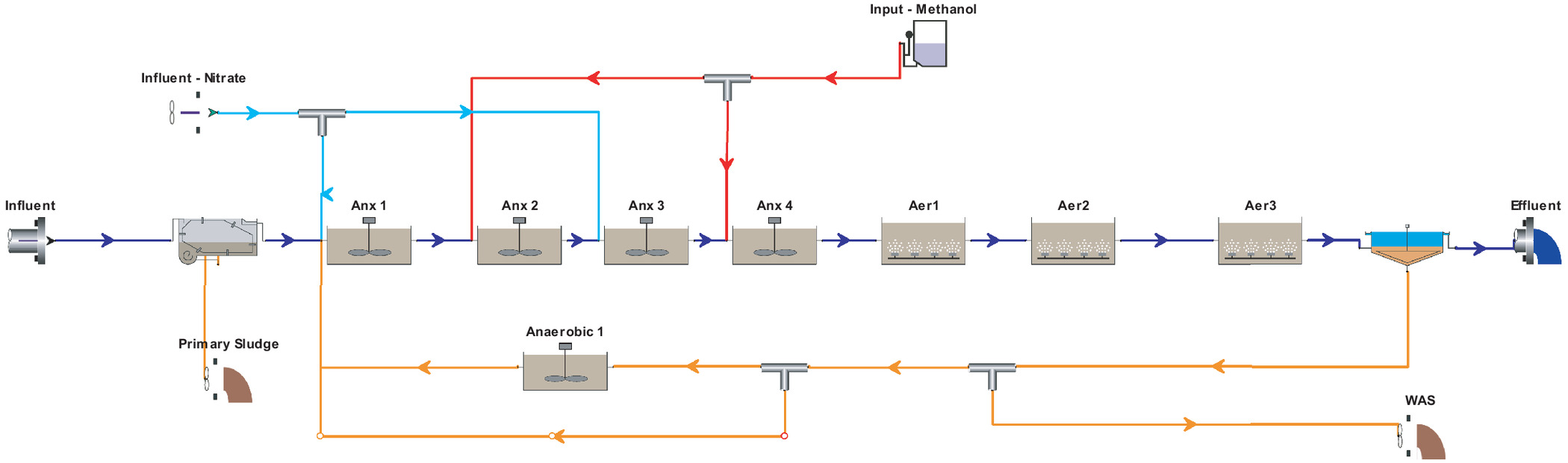
These simulations used a 24-h anaerobic and 20% of the RAS flow. Particulate COD constituted the largest fraction of COD, with less than 1% as readily biodegradable COD. The simulations showed that the addition of fermentation resulted in a negligible improvement in effluent TN removal. For example, methanol dosing without fermentation resulted in an effluent TN of , whereas the combination of the same dose of methanol with fermentation resulted in an effluent TN of . Thus, the sidestream reactor was not considered further in this study.
Optimization Results
Based on the preliminary simulations described previously, the nitrate step-feed process with methanol addition configuration [Fig. 2(c)] had the lowest effluent TN concentration and therefore was selected for numerical optimization.
Sixty iterations of the numerical optimization procedure (Fig. 1) were required to meet the convergence criteria. The initial value for the objective function was $30,947/d, and the final value was $14,331/d (Fig. 4), for a 54% reduction in overall daily cost. There was a reduction in bioreactor volume from 35,280 to (Fig. 5), which results in a reduction in total HRT from 17.2 to 8.2 h. The final effluent TN was , and the concentration was , which was within the desired effluent concentration constraint of less than . The methanol dosage was removed. This compares to typical values of 3.3 to removed (Metcalf and Eddy 2014).
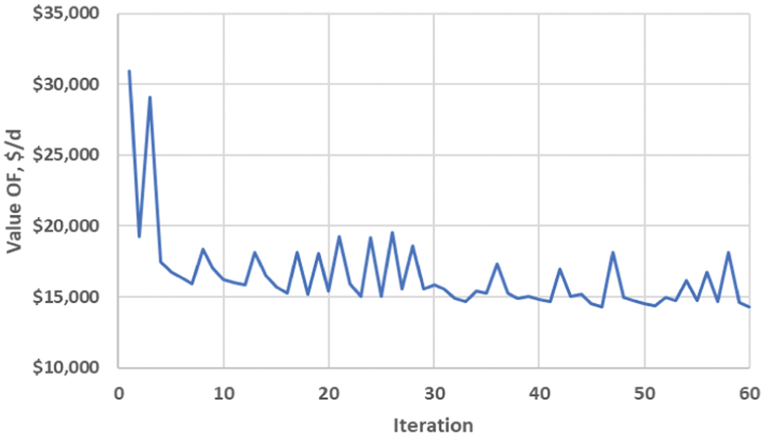
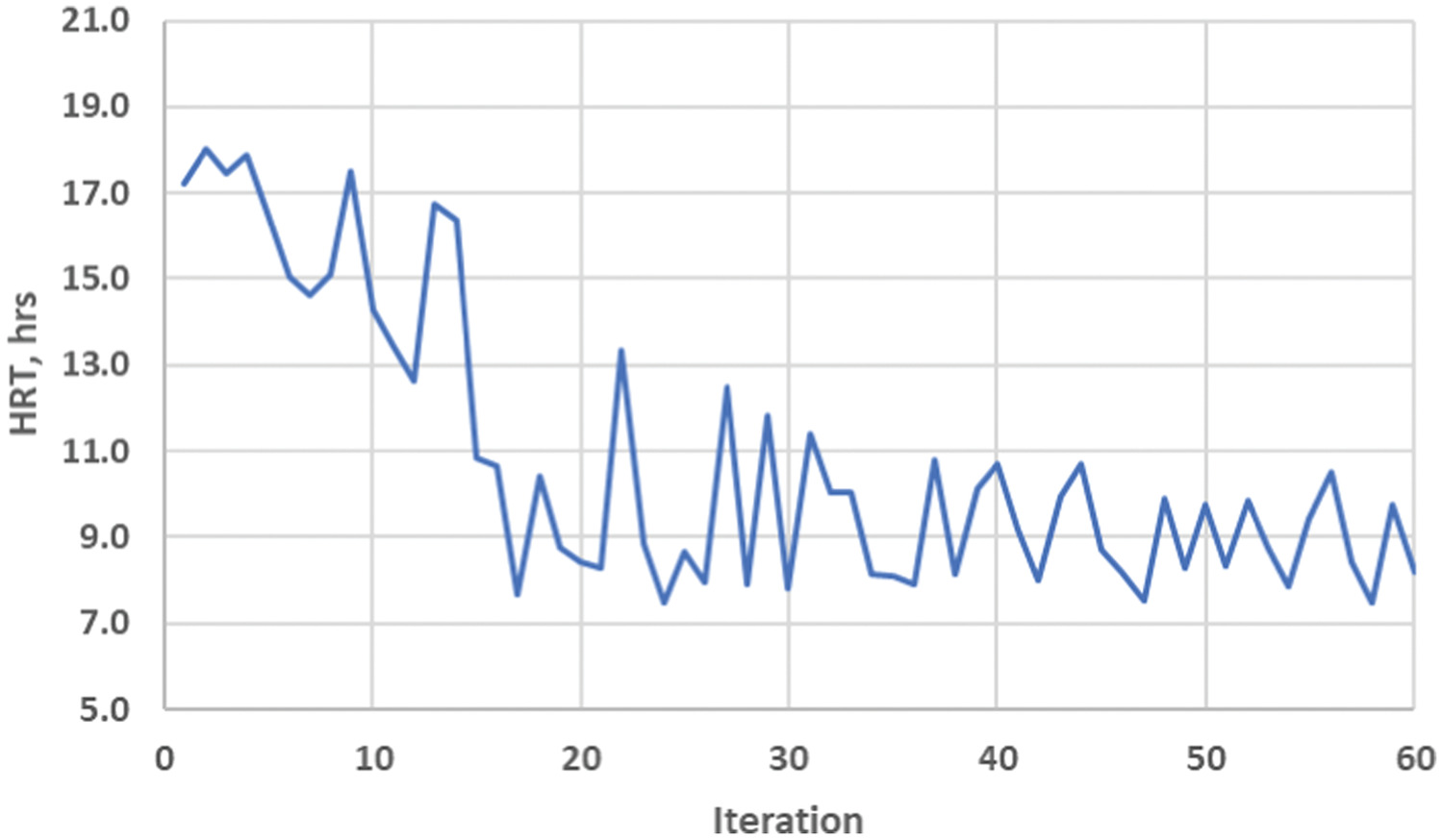
Table 5 is a summary of the input variables and the simulation results for the final optimized design. Table 6 shows the cost for each of the OF elements for the optimal design and the percentage each contributes to the overall cost. It can be seen that the factors that contribute most to the costs are the size of the reactor, solids disposal, and methanol supplementation. These add to 72.7% of the total objective function costs. A further 14.1% of the cost is attributable to a penalty for total Kjeldahl nitrogen (TKN) in the effluent.
| Input variable | Value | Parameter | Value |
|---|---|---|---|
| Nitrate waste flow zone 1, % | 50.00 | SRT (days) | 11.6 |
| Anoxic HRT 1 (h) | 2.00 | () | 5.0 |
| Anoxic HRT 2 (h) | 1.10 | () | 3.8 |
| Anoxic HRT 3 (h) | 0.60 | () | 1.3 |
| Anoxic HRT 4 (h) | 7.90 | TKN () | 3.8 |
| Aerobic HRT (h) | 5.70 | TN () | 12.6 |
| Total HRT (h) | 17.30 | BOD () | 4.4 |
| Internal recycle ratio | 3.60 | TSS () | 8.0 |
| WAS flow ratio | 0.01 | — | — |
Note: Nitrate Waste Flow Zone 1 is the fraction of nitrate waste added to the first reactor. The HRT, internal recycle ratio, and WAS flow ratio are all relative to the domestic wastewater flow rate plus the industrial flow rate: .
| Element | Percentage | Cost, |
|---|---|---|
| Reactor cost | 25.3 | 2,806 |
| MeOH cost | 22.6 | 3,234 |
| Clarifier cost | 2.5 | 357 |
| Aeration cost | 1.6 | 229 |
| Internal recycle | 0.7 | 101 |
| BOD + TSS | 0.7 | 98 |
| TKN penalty | 14.1 | 2,016 |
| Nitrate penalty | 4.9 | 698 |
| Nitrite penalty | 2.9 | 419 |
| Solids disposal | 24.8 | 3,552 |
Conclusions and Next Steps
The results of this study indicate that industrial waste with a high nitrate concentration has the potential to be economically treated using carbon from municipal wastewater to reduce the need for supplemental carbon dosage. Furthermore, the coupling of the external biological models with the Nelder–Mead optimization algorithm indicates that substantial capital and operating costs savings can be achieved in the design process. This research was unique in the coupling of an external biological simulation model with a numerical optimization algorithm to minimize total costs including those related to design, operation, and performance. This approach has the potential to significantly improve the cost effectiveness of wastewater treatment design and operation in practice.
Although the steps of the optimization procedure as shown in Fig. 1 were conducted by manually communicating data from one program to the next, it is recommended that ASM simulation programs be modified to incorporate calculation of the objective function and the Nelder–Mead calculation in order to automate the approach developed in this work. Also, it is recommended that the simulation incorporate variability in diurnal and seasonal influent characteristics so that the range of process performance results could be evaluated. Therefore, the next step in this study (which is underway) is to design, construct, and operate a pilot system located at a WRRF using actual wastewater influent to the reactor to validate this concept.
Appendix. Nelder–Mead Code
This appendix shows the MATLAB code used for the Nelder–Mead optimization process.
| % Nelder-Mead Interactive Experiment Guide |
| % by Carlo Vaccari |
| % and David A. Vaccari |
| % Stevens Institute of Technology |
| alpha = 1.0; %reflect factor |
| gamma = 2.0; %expand factor |
| rho = 0.5; %contract factor |
| sigma = 0.5; %shrink factor |
| varCount = input(“Number of independent variables: ”); |
| threshold = input(“Enter convergence tolerance: ”); |
| iVars = zeros(varCount+1, varCount); |
| disp(“Entering the coordinates of opposite corners of a hypercube will be”) |
| disp(“ used to define the starting simplex for Nelder-Mead optimization.”) |
| disp(“ The first set will be the low values for each independent variable.”) |
| disp(“ The second set will be the high values for each independent variable.”) |
| disp(“ ”) |
| disp(“Enter first (low values) set of independent variables:”) |
| for i=(1:varCount) |
| iVars(:,i) = input(strcat(“Independent variable %”,int2str(i),“: ”)); |
| end%for |
| disp(“ ”) |
| disp(“Enter second (high values) set of variables:”) |
| for i=(1:varCount) |
| iVars(i+1,i) = input(strcat(“Independent variable %”,int2str(i),“: ”)); |
| end%for |
| results = zeros(varCount+1,1); |
| for i=(1: varCount+1) |
| disp(“ ”) |
| disp(“Enter result for experiment with the following variables:”) |
| for varNum=(1:varCount) |
| disp(strcat(“Independent variable %”,int2str(varNum),“: ”,num2str(iVars(i,varNum)))) |
| end%for |
| results(i) = input(“Result: ”); |
| end%for |
| step = 0; |
| while true |
| worst = max(results); |
| worstIndex = find(results==worst,1); |
| worstPoint = iVars(worstIndex,:); |
| best = min(results); |
| bestIndex = find(results==best,1); |
| bestPoint = iVars(bestIndex,:); |
| MaxDiff = worst-best |
| disp(strcat(“Worst-Best = ”,num2str(MaxDiff))) |
| % Choose one of the following termination criteria: |
| % (Make sure one and only one is commented out) |
| if (MaxDiff < threshold) %First termination criterion |
| % if (best < threshold) %Second termination criterion |
| break |
| end%if |
| sortedResults = sort(results); |
| centroid = zeros(1,varCount); |
| for i=(1:varCount+1) |
| if (i ∼= worstIndex) |
| centroid=centroid+iVars(i,:)); |
| end%if |
| end%for |
| centroid = centroid/varCount; |
| % Reflection |
| reflectPoint = centroid+alpha*(centroid-worstPoint); |
| disp(“ ”) |
| step = step+1; |
| disp(strcat(“Step ”,int2str(step))) |
| disp(“Enter result for experiment with the following variables (reflected):”) |
| for varNum=(1:varCount) |
| disp(strcat(“Independent variable %”,int2str(varNum),“: ”,num2str(reflectPoint(varNum)))) |
| end%for |
| reflectResult = input(“Result: ”); |
| if (reflectResult < sortedResults(varcount))%If reflected is better than second-worst |
| if (reflectResult > best) %and worse than best |
| %then replace worst point with reflected. |
| iVars(worstIndex,:) = reflectPoint; |
| results(worstIndex) = reflectResult; |
| continue; |
| else %Check whether to expand. |
| expandPoint = centroid+gamma*(centroid-worstPoint); |
| disp(“ ”) |
| step=step+1; |
| disp(strcat(“Step ”,int2str(step))) |
| disp(“Enter result for experiment with the following variables (expanded):”) |
| for varNum=(1:varCount) |
| disp(strcat(“Independent variable %”,int2str(varNum),“: ”,num2str(expandPoint(varNum)))) |
| end%for |
| expandResult = input(“Result: ”); |
| if (expandResult < reflectResult)% Expanded is better than reflected |
| %expand |
| iVars(worstIndex,:) = expandPoint; |
| results(worstIndex) = expandResult; |
| else |
| %reflect |
| iVars(worstIndex,:) = reflectPoint; |
| results(worstIndex) = reflectResult; |
| end%if |
| end%if |
| else %reflect is still worse than second-worst |
| %contract to centroid? |
| contractPoint = centroid+rho*(worstPoint-centroid); |
| disp(“ ”) |
| step=step+1; |
| disp(strcat(“Step ”,int2str(step))) |
| disp(“Enter result for experiment with the following variables (contract):”) |
| for varNum=(1:varCount) |
| disp(strcat(“Independent variable %”,int2str(varNum),”: ”,num2str(contractPoint(varNum)))) |
| end%for |
| contractResult = input(“Result: ”); |
| if (contractResult < worst)%contract is better than worst |
| %contract |
| iVars(worstIndex,:) = contractPoint; |
| results(worstIndex) = contractResult; |
| else |
| %shrink about best |
| for i=1:varCount+1 |
| if (i ∼= bestIndex) |
| iVars(i,:) = bestPoint+sigma*(iVars(i,:)-bestPoint); |
| disp(“ ”) |
| step=step+1; |
| disp(strcat(“Step ”,int2str(step))) |
| disp(“Enter result for experiment with the following variables (shrink):”) |
| for varNum=(1:varCount) |
| disp(strcat(“Independent variable %”,int2str(varNum),“: ”,num2str(iVars(i,varNum)))) |
| end%for |
| results(i) = input(“Result: ”); |
| end%if |
| end%for |
| end%if |
| end%if |
| end%while |
| disp(“ ”) |
| disp(strcat(“DONE. Best result: ”,num2str(best))) |
| for i=1:varCount |
| disp(strcat(“Optimal independent variable %”,int2str(i),“: ”,num2str(bestPoint(i)))) |
| end%for |
Data Availability Statement
All data, models, or code that support the findings of this study are available from the corresponding author upon reasonable request (BioWin simulation results, Nelder–Mead simulation results, Excel optimization spreadsheets).
Acknowledgments
The project was supported by the Center for Environmental Systems, Stevens Institute of Technology.
References
Alvarez-Vázquez, L. J., A. Martínez, C. Rodríguez, and M. E. Vázquez-Méndez. 2002. “Numerical optimization for the location of wastewater outfalls.” Comput. Optim. Appl. 22 (3): 399–417. https://doi.org/10.1023/A:1019767123324.
Barnard, J. L. 2006. “Biological nutrient removal: Where we have been, where we are going?” In Proc., Water Environment Federation, 1–25. Alexandria, VA: Water Environment Federation.
Chen, W., H. Dai, T. Han, X. Wang, X. Lu, and C. Yao. 2020. “Mathematical modeling and modification of a cycle operating activated sludge process via the multi-objective optimization method.” J. Environ. Chem. Eng. 8 (6): 104470. https://doi.org/10.1016/j.jece.2020.104470.
Chen, W., C. Yao, and X. Lu. 2014. “Optimal design activated sludge process by means of multi-objective optimization: Case study in Benchmark Simulation Model 1 (BSM1).” Water Sci. Technol. 69 (10): 2052–2058. https://doi.org/10.2166/wst.2014.119.
CTNCAB (Connecticut Nitrogen Credit Advisory Board). 2021. “Buyers and sellers.” Accessed September 10, 2021. https://portal.ct.gov/DEEP/Municipal-Wastewater/Nitrogen-Credit-Advisory-Board/Nitrogen-Credit-Advisory-Board.
Cyplik, P., R. Marecik, A. Piotrowska-Cyplik, A. Olejnik, A. Drożdżyńska, and Ł. Chrzanowski. 2012. “Biological denitrification of high nitrate processing wastewaters from explosives production plant.” Water Air Soil Pollut. 223 (May): 1791–1800.
Dai, H., W. Chen, and X. Lu. 2016. “The application of multi-objective optimization method for activated sludge process: A review.” Water Sci. Technol. 73 (2): 223–235. https://doi.org/10.2166/wst.2015.489.
Daigger, G. T. 2011. “A practitioner’s perspective on the uses and future developments for wastewater treatment modeling.” Water Sci. Technol. 63 (3): 516–526. https://doi.org/10.2166/wst.2011.252.
Daigger, G. T., and D. Nolasco. 1995. “Evaluation and design of full-scale wastewater treatment plants using biological process models.” Water Sci. Technol. 31 (2): 245–255. https://doi.org/10.2166/wst.1995.0112.
De Filippis, P., L. Di Palma, M. Scarsella, and N. Verdone. 2013. “Biological denitrification of high-nitrate wastewaters: A comparison between three electron donors.” Chem. Eng. 32 (2013): 319–324.
Dhamole, P. D., R. R. Nair, S. F. D’Souza, and S. S. Lele. 2007. “Denitrification of high strength nitrate waste.” In Bioresource technology. Amsterdam, Netherlands: Elsevier.
Dubrovsky, N. M., et al. 2010. The quality of our nation’s waters—Nutrients in the nation’s streams and groundwater, 1992–2004. Washington, DC: USGS.
EIA (Energy Information Administration). 2021. “US electricity profile 2021.” Accessed September 10, 2021. https://www.eia.gov/electricity/data/state/.
Fernández-Nava, Y., E. Maranon, J. Soons, and L. Castrillon. 2008. “Denitrification of wastewater containing high nitrate and calcium concentrations.” In Bioresource technology. Amsterdam, Netherlands: Elsevier.
Glass, C., and J. Silverstein. 1999. “Denitrification of high-nitrate, high-salinity wastewater.” Water Res. 33 (1): 223–229.
Hakanen, J., K. Sahlstedt, and K. Miettinen. 2013. “Wastewater treatment plant design and operation under multiple conflicting objective functions.” Environ. Modell. Software 46 (Aug): 240–249. https://doi.org/10.1016/j.envsoft.2013.03.016.
Henze, M., W. Gujer, T. Mino, and M. C. van Loosdrecht. 2006. Activated sludge models ASM1, ASM2, ASM2d and ASM3. London: IWA.
Khoja, I., T. Ladhari, A. Sakly, and F. M’sahli. 2018. “Parameter identification of an activated sludge wastewater treatment process based on particle swarm optimization method.” Math. Probl. Eng. 2018 (Oct): 1–11. https://doi.org/10.1155/2018/7823930.
Kim, D., J. D. Bowen, and E. C. Ozelkan. 2015. “Optimization of wastewater treatment plant operation for greenhouse gas mitigation.” J. Environ. Manage. 163 (Nov): 39–48. https://doi.org/10.1016/j.jenvman.2015.07.005.
Ludwig, T., P. Kern, M. Bongards, and C. Wolf. 2011. “Simulation and optimization of an experimental membrane wastewater treatment plant using computational intelligence methods.” Water Sci. Technol. 63 (10): 2255–2260. https://doi.org/10.2166/wst.2011.135.
MathWorks. 2008. MATLAB 7, function reference. Natick, MA: MathWorks.
Metcalf and Eddy. 2014. Wastewater engineering: Treatment and reuse. 5th ed. New York: McGraw-Hill.
Mohan, T. K., Y. V. Nancharaiah, V. P. Venugopalan, and P. S. Sai. 2016. “Effect of C/N ratio on denitrification of high-strength nitrate wastewater in anoxic granular sludge sequencing batch reactors.” Ecol. Eng. 91 (Jun): 441–448.
Nelder, J. A., and R. Mead. 1965. “A simplex method for function minimization.” Comput. J. 7 (4): 308–313. https://doi.org/10.1093/comjnl/7.4.308.
NYC (New York City). 2021. “A new way to dispose of NYC’s sewage biosolids can save money and counter the climate crisis at the same time—but needs support from NYC and NY State agencies and legislators.” Accessed August 8, 2021. https://www.beyondoilnyc.org/lowering-nyc-waste-costs.
Onnis-Hayden, A., V. Srinivasan, N. B. Tooker, G. Li, D. Wang, J. L. Barnard, and A. Z. Gu. 2020. “Survey of full-scale sidestream enhanced biological phosphorus removal (S2EBPR) systems and comparison with conventional EBPRs in North America: Process stability, kinetics, and microbial populations.” Water Environ. Res. 92 (3): 403–417. https://doi.org/10.1002/wer.1198.
Rafati, M., M. Pazouki, H. Ghadamian, A. Hossein Nia, and A. Jalilzadeh. 2022. “Determine the most effective process control parameters on activated sludge based on particle swarm optimisation algorithm.” Int. J. Environ. Anal. Chem. 102 (19): 7595–7616. https://doi.org/10.1080/03067319.2020.1836169.
Scholarpedia. 2009. “Nelder-Mead algorithm.” Accessed April 14, 2021. http://www.scholarpedia.org/article/Nelder-Mead_algorithm.
Shen, J., R. He, W. Han, X. Sun, J. Li, and L. Wang. 2009. “Biological denitrification of high-nitrate wastewater in a modified anoxic/oxic-membrane bioreactor (A/O-MBR).” J. Hazard. Mater. 172 (2–3): 595–600.
USEPA. 2009. “Circular economy.” Accessed August 9, 2021. https://www.epa.gov/recyclingstrategy/what-circular-economy.
USEPA. 2015. “A compilation of cost data associated with the impacts and control of nutrient pollution.” Accessed August 9, 2021. https://www.epa.gov/sites/production/files/2015-04/documents/nutrient-economics-report-2015.pdf.
USEPA. 2022a. “2022 EPA nutrient reduction memorandum.” Accessed July 9, 2022. https://www.epa.gov/nutrient-policy-data/2022-epa-nutrient-reduction-memorandum.
USEPA. 2022b. “The issue.” Accessed July 9, 2022. https://www.epa.gov/nutrientpollution/issue.
USEPA. 2022c. “Criminal provisions.” Accessed August 9, 2021. https://www.epa.gov/enforcement/criminal-provisions-water-pollution.
Zhang, R., W. Xie, H. Yu, and W. Li. 2014. “Optimizing municipal wastewater treatment plants using an improved multi-objective optimization method.” Bioresour. Technol. 157 (2014): 161–165.
Information & Authors
Information
Published In

Journal of Environmental Engineering
Volume 149 • Issue 12 • December 2023
Copyright
This work is made available under the terms of the Creative Commons Attribution 4.0 International license, https://creativecommons.org/licenses/by/4.0/.
History
Received: Feb 13, 2023
Accepted: Jul 21, 2023
Published online: Oct 11, 2023
Published in print: Dec 1, 2023
Discussion open until: Mar 11, 2024
ASCE Technical Topics:
- Analysis (by type)
- Buildings
- Engineering fundamentals
- Environmental engineering
- Facilities (by type)
- Industrial facilities
- Industrial wastes
- Municipal wastes
- Municipal wastewater
- Numerical analysis
- Pollutants
- Solid wastes
- Structural engineering
- Structures (by type)
- Waste management
- Waste treatment
- Waste treatment plants
- Wastes
- Wastewater management
- Wastewater treatment plants
- Water treatment
- Water treatment plants
Authors
Metrics & Citations
Metrics
Citations
Download citation
If you have the appropriate software installed, you can download article citation data to the citation manager of your choice. Simply select your manager software from the list below and click Download.