Enhancing the Evaporation Method for Accurately Determining Unsaturated Soil Properties in the Wet Range
Publication: Journal of Hydrologic Engineering
Volume 29, Issue 6
Abstract
The evaporation (EV) method is a widely used experimental approach to determine unsaturated hydraulic conductivity (UHC) and soil water retention (SWR) functions. However, the EV method has some limitations in evaluating accurate UHC values near the wet range. This restricts the working range of the models that utilize these UHC values for predicting soil water content and water fluxes for problems involving wet conditions (e.g., infiltration under ponding conditions). Our experimental study shows that when using the EV method, tensiometer offset errors as low as 1 cm can cause problems with wet-range measurements. Current methods to overcome these errors are expensive, inefficient, or cumbersome. In this study, we developed an improved EV method that utilizes a simple experimental protocol for standardizing the soil saturation procedure and a robust calibration method to quantify tensiometer offset errors. The proposed approach utilizes existing EV method hardware without requiring additional specialized instrumentation. Experiments performed using a silt loam soil sample show that our approach can extend the working range of the EV method to the wet range. Therefore, reliable estimates of the UHC and SWR functions can now be obtained over the entire range of soil suction heads. Our study also contributes to a better understanding of the EV method and uses this knowledge for collecting reliable and reproducible SWR and UHC data. The improved EV method is simple, effective, and cost-efficient. This method has the potential to greatly improve soil water content predictions, leading to better-informed decisions for groundwater resources management, sustainable agriculture, and environmental protection.
Introduction
The evaporation (EV) method is one of the most efficient methods available for estimating unsaturated soil properties (Wind 1968). The EV method, also known as the Wind method, essentially records volumetric water content and matric potential data at different times as a soil sample is allowed to dry via surface evaporation. By analyzing these data using an analytical procedure, one can construct both soil water retention (SWR) and unsaturated hydraulic conductivity (UHC) functions. Over the years, various experimental modifications and data analysis methods have been proposed to improve the EV method (Schindler 1980; Wendroth et al. 1993; Schindler and Müller 2006).
Schindler (1980) proposed a widely adopted variant of the EV method, which uses changes in the soil weight and the value of matric potential measured at two points to develop SWR and UHC functions. The data analysis procedure assumes linear variation in water flux within the soil sample (Schindler and Müller 2006), an assumption that is valid for matric potential values up to 1,000 cm (Schindler et al. 2010a; Peters et al. 2015). In the early years, the applicability range of the EV method was limited primarily by the cavitation limit of the tensiometers. Schindler et al. (2010b) used improved tensiometers fitted with a porous ceramic cup, that avoided early cavitation, to extend the pressure range. Schindler et al. (2010a) later refined the method by using degassed water in the tensiometer to further delay cavitation. Schindler et al. (2012) conducted a validation study in which they compared the SWR curves obtained using both the classic equilibrium method and the EV method and concluded that both methods produced comparable results.
However, the UHC function developed using the EV method has some limitations because the UHC data collected near the wet range tend to have considerable variation (Wendroth et al. 1993; Tamari et al. 1993; Schindler et al. 2010b). These variations are due primarily to tensiometer measurement errors (Wendroth et al. 1993; Tamari et al. 1993; Peters and Durner 2008). Peters and Durner (2008) used synthetic data sets to demonstrate numerically how tensiometer offset errors can lead to erroneous overestimation (referred to here as Case 1) or underestimation (referred to here as Case 2) of UHC values. To address this problem, they proposed a rejection criterion to discard UHC data collected near the wet range. However, applying the criterion often results in discarding more than 50% of measured data points, potentially yielding unrealistic UHC functions. Fig. 1(a) illustrates the overestimation problem (Case 1), in which the data have an overestimation trend. In Fig. 1(a), taken from Peters and Durner (2008), the overshoot extends up to a matric potential of about 100 cm because Peters and Durner (2008) discarded the unstable data collected near the wet range (matric potential values below 70 cm) by applying data rejection criteria. Even after rejection, the data points trend toward unrealistic high values and form a distinctly different shape compared with the expected UHC function that was fitted to the van Genuchten–Mualem (van Genuchten 1980) function using the remaining data. The theoretical model–based data clearly exhibit a downward trend, in contrast to the experimental data that have an upward trend.
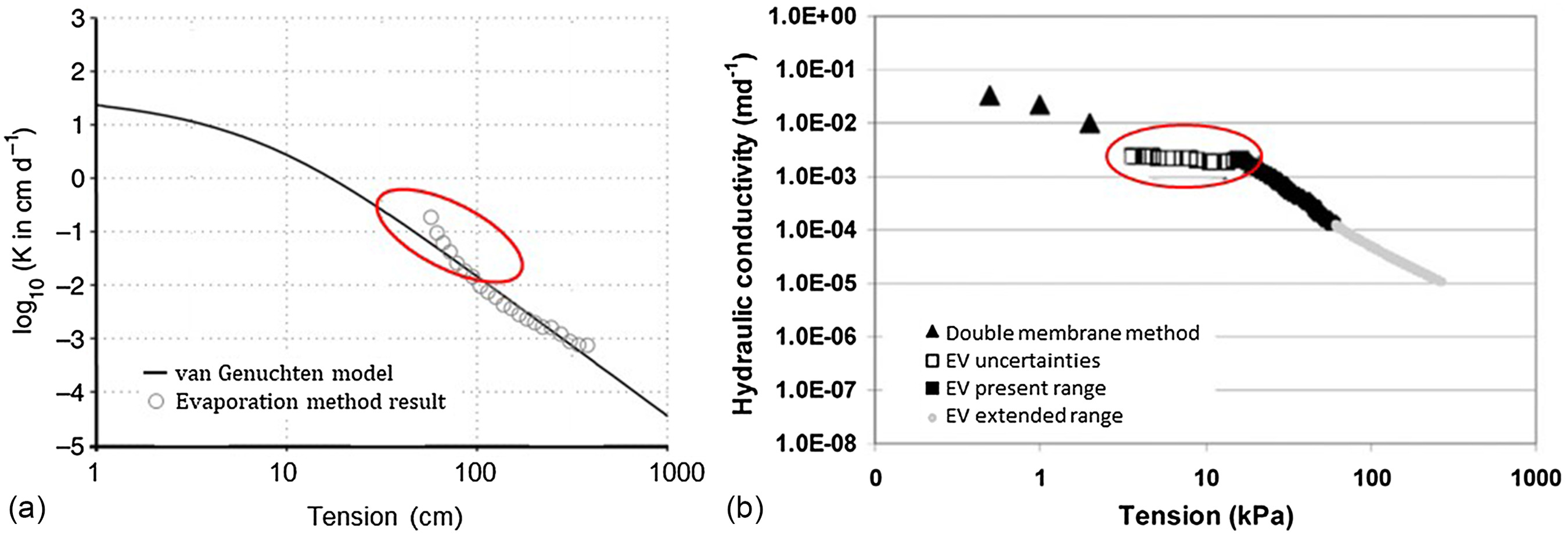
Fig. 1(b) presents an example of UHC underestimation error (Case 2). In this case, before applying the rejection criterion, the EV method yielded abnormally low and flat data points in the wet range [Fig. 1(a), hollow squares]. Because the UHC values in the wet range are important for modeling rapid soil water transport near the wet range (Ahuja et al. 1995; Schindler et al. 2010b), researchers have combined the EV method with other techniques to collect data in the wet range. These methods include the use of an advanced differential transducer setup (Masaoka and Kosugi 2018), double-membrane method (Henseler and Renger 1969; Klute 1972; Boels et al. 1978; Wendroth and Simunek 1999; Schindler et al. 2010a), or multistep-outflow methods (Fujimaki and Inoue 2003; Schelle et al. 2011), to name a few. Schindler et al. (2010a) used the double-membrane method to collect the wet range data [Fig. 1(b), triangles]. However, such combined methods require additional experimental procedures and specialized equipment. Therefore, to maintain simplicity, researchers often prefer using the EV method alone, and simply exclude the wet-range data (Inforsato et al. 2023; Liu et al. 2021; Bezerra-Coelho et al. 2018).
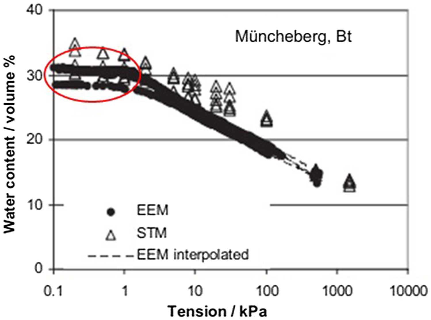
UHC and SWR functions also are susceptible to other experimental errors (Mohrath et al. 1997; Peters and Durner 2008; Breitmeyer and Fissel 2017), some of which can be attributed to sample preparation procedures used for saturating the soil. Incomplete saturation often results in residual air trapped in the soil, which can significantly impact unsaturated hydraulic properties (Machaček et al. 2023; Sakaguchi et al. 2005; Stonestrom and Rubin 1989; Kaluarachchi and Parker 1987), leading to poor reproducibility and other undesirable variations in measured data (van Schaik and Laliberte 1969). Fig. 2 presents two SWR data sets collected by Schindler et al. (2012) for the same soil, which have considerable variation, particularly near the wet range [Fig. 2, extended evaporation method (EEM) data]. Standardizing the soil preparation procedure to fully saturate the soil can help mitigate this problem (Sakaguchi et al. 2005).
This paper presents an experimental protocol that systematically quantifies and corrects tensiometer errors when using the EV method, thereby eliminating the need for a rejection criterion to remove wet-range data. In addition, we also propose a systematic sample preparation procedure that can help collect reproducible, high-quality UHC and SWR data under both wet and dry conditions.
Materials and Method
Experimental Setup
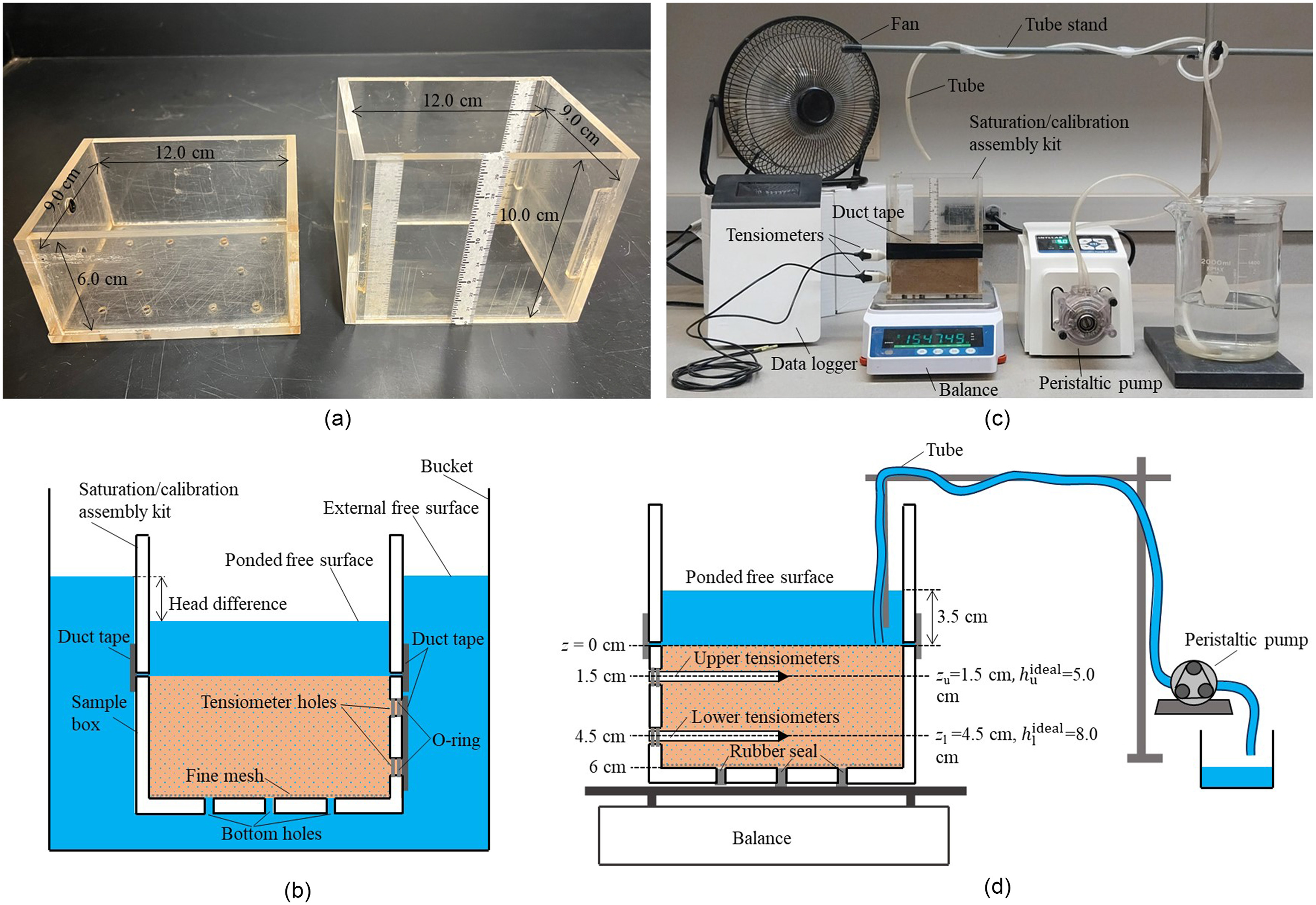
Fig. 3(a) shows the plexiglass sample box (left) and a saturation–calibration assembly kit (right) that we used to conduct all our EV experiments. The internal dimensions of the sample box were . In addition to the sample box, we also used the saturation–calibration assembly kit, which allowed us to properly saturate the soil and collect data for calibrating the tensiometers that were placed directly within the sample (the details of which are discussed subsequently). The dimensions of the saturation–calibration assembly kit were ; it was composed of four sides without a bottom). The bottom of the sample box was equipped with 10 4.5-mm holes. A fine mesh was placed at the bottom of the box to prevent soil from washing out. The bottom holes were used for saturating the soil, but they could be sealed at any time using small rubber caps to prevent leakage. Two miniature tensiometers [TEROS 31, METER Group (Pullman, Washington)] were installed in the sample box via predrilled tensiometer holes in the front face of the sample box [Fig. 3(b)]. Two rubber O-rings were installed at each hole to ensure a proper seal to prevent water leakage and to guide the horizontal installation of the tensiometers (which measure pressure at their ceramic tips). The top and bottom tensiometers were placed at 1.5 and 4.5 cm below the top of the sample box (and the surface of the soil sample), respectively, which corresponded to about 25% and 75% of the sample’s height. The measurement range of the tensiometers used in the experiment was to 50 kPa, which enabled precise measurement of both positive and negative pressures (the positive pressure data were utilized subsequently for tensiometer calibration). Our design is similar to the setup used by Schindler and Müller (2006). For data acquisition, we used a ZL6 system (METER Group) to record the tensiometer data. Both tensiometer and sample weight data were collected every 30 min. In addition, we independently measured the value of saturated hydraulic conductivity after conducting multiple experiments (seven times) using the falling head method.
Sample Preparation and Saturation Procedure
The quality of data collected during the initial times (in the wet range) is highly dependent on the initial condition of the saturated soil sample. Achieving uniform and complete saturation across the entire sample can be a challenging task. This is because the degree of saturation can vary based on the sample packing condition and the techniques used for saturating the sample. In this study, we employed the following protocol to ensure uniformity in packing and consistency in the initial saturation level.
The soil material selected for this study was Tuscaloosa silt loam soil purchased from a local sand quarry in Tuscaloosa, Alabama. The soil was dried for 24 h in an oven at 105°C to remove all moisture. The dry soil sample was layered into the sample box in three equal layers with vibratory compaction (manually vibrating the sample by tapping it on a flat surface). When the sample box was filled, the mass of the sample (dry weight of the soil sample) was measured. After the packing step, a careful saturation procedure was employed to fully saturate the soil sample. In the published literature, others have used a bottom-up saturation procedure by placing samples in a water pan and letting the water slowly rise from approximately 0.5 cm above the sample bottom to about 0.2 mm below the sample surface, to minimize air entrapment (Schindler et al. 2010a). However, we found that achieving complete saturation can be a challenging task using this method, particularly for low-hydraulic-conductivity soils.
To achieve full saturation, we first increased the height of the sample box walls by placing the saturation–calibration assembly kit [Fig. 3(b)]. To prevent leakage, both the saturation–calibration assembly kit and the sample box were secured together using duct tape. The entire setup including the sample box attached to the saturation–calibration assembly kit then was placed in a bucket of water [Fig. 3(b)]. Using a peristaltic pump, we gradually raised the water level in the bucket. As the external free surface began to rise, the water level inside the sample box also started to rise, allowing the water to enter through the holes at the bottom of the sample box. The exterior free surface was raised gradually over 24 h until the free surface of the ponded water inside the sample box (ponded free surface) was approximately 2 cm below the external free surface [Fig. 3(b)]. This procedure was used to force the water to seep from the bottom of the sample box, slowly replacing the air. In this step, it was crucial to continuously maintain a low head difference between the internal and external free surfaces to prevent soil boiling, sample expansion, or air-trapping problems. When the soil was fully saturated, the sample box was removed from the bucket. Rubber seals were used to plug the bottom holes to prevent water drainage. After the sample was removed from the bucket, the soil continued to remain submerged under ponded water (the free surface was about 3.5 cm above soil the soil surface) in the assembly [Fig. 3(d)]. This ponding initial condition was required for the tensiometer calibration procedure used in this study.
Data Analysis Procedure for the Evaporation Method
In Schindler’s EV method, the spatially averaged value (averaged over the entire sample) of volumetric water content, , and the average of matric potential values measured at two different depths, , are used to obtain the data needed for developing the SWR function (Schindler and Müller 2006). The average volumetric water content, , is computed by determining the soil water volume, based on the mass of the soil sample (assuming 1 g of ). This calculated water volume is divided by the volume of the soil sample to determine the volumetric water content. The average matric potential, , is calculated as the arithmetic mean of the two matric potential values, and , measured at two different depths, and (where , and , where is the total height of the soil sample). Continuous monitoring of weight changes and matric potential allows one to track the temporal changes of and values as the system loses water over time due to evaporation.
The EV method is based on the assumption that the flux varies linearly with a maximum value at the top and zero at the bottom. Therefore, the flux at the midpoint of the sample should be half the maximum flux. After invoking this assumption, UHC values can be calculated by applying the Darcy–Buckingham law at each measurement time interval (Schindler 1980)where = measurement time interval between two consecutive times, and ; = mean matric potential measured by the upper tensiometer at position and the lower tensiometer at position , averaged over the time interval ( is the average of four individual measurements); = evaporated water volume, which is obtained by dividing the mass, , lost over time interval by the density of water, ; and = cross-sectional area of the sample. The average hydraulic gradient, , experienced by the system over the time interval is estimated using the matric potential measured by the upper and lower tensiometers ( and , respectively) at two consecutive times, and , aswhere is the vertical coordinate, which is assumed to be positive in the downward direction. Furthermore, in Eqs. (2)–(4), we used the negative matric potential values measured for the unsaturated soil system.
(1)
(2)
(3)
(4)
Tensiometer Calibration Procedure
Errors in tensiometer readings inevitably are included in the calculation of hydraulic gradients [i.e., Eqs. (2) and (3)]. We calibrated the tensiometer readings directly on the sample under hydrostatic conditions by establishing ponded water above the soil surface, ensuring hydrostatic conditions that are supposed to yield zero hydraulic gradient [Eqs. (2) and (3)]. We placed the saturated sample with ponded water on the balance and installed the tensiometer and the peristaltic pump tube as shown in Fig. 3(d). We ensured that the tube was in direct contact with the soil surface so that all the ponded water would be pumped out. We first let the system reach the initial ponded-equilibrium condition and recorded the tensiometer value. We then started the peristaltic pump to remove the ponded water. The pumping rate was set to a low value to decrease the ponded free surface at the rate of about . Throughout this process, we recorded the tensiometer readings (pressure data) and actual values (estimates for hydrostatic conditions), which subsequently were used for tensiometer calibration. This method, which was applied directly to the sample, allowed us to avoid any separate calibration procedures. Furthermore, by using this method we were able to collect continuous pressure data as the system seamlessly transitioned from measuring positive to negative pressures. After pumping out all the ponded water, we quickly removed the tube and turned on the fan to start the evaporation experiment.
We corrected the upper and lower tensiometer readings ( and ) after accounting for the offset errors in the upper and lower tensiometers (i.e., and ). The offset errors can be defined by fitting the tensiometer readings (ℎ) to the actual values () using the following equations:where and denote upper and lower tensiometers, respectively [Fig. 3(d)]. Although the measured offset errors were relatively small, they had a substantial influence on the quality of the initial data, near the wet range. We adapted Eqs. (2) and (3) to compute the true gradient values after making appropriate correction as follows:where () = net offset error, which can be either positive or negative, leading to classification as either a net-positive offset or a net-negative offset. The implications of these classifications and their respective impacts on the experimental results are discussed in the “Results and Discussion” section.
(5)
(6)
(7)
(8)
Experimental Design
We first completed the proposed tensiometer calibration step to quantify the tensiometer offset error. This procedure estimated the magnitude of the offset error in both tensiometers, and also determined whether the net offset error was positive or negative. We then conducted the EV experiment to generate a baseline experimental data set after implementing proper tensiometer corrections (referred to here as Experiment 1 or Corrected data set). Subsequently, this baseline data set also was used to develop two derived data sets, details of which are discussed subsequently. We replicated the EV experiment two more times (referred to here as Experiments 2 and 3) using the same soil, and thus collected a total of three distinct data sets to test the reproducibility of the experimental results.
Results and Discussion
Quantifying Tensiometer Offset Error
Fig. 4 presents the tensiometer calibration data obtained using the calibration procedure directly on the sample. The data in Fig. 4 employed ponded conditions with the initial free surface set at 3.5 cm above the soil surface. Because the upper and lower tensiometers were installed at 1.5 and 4.5 cm below the soil surface, the initial actual values (estimates based on hydrostatic conditions) of the tensiometers should have been 5.0 and 8.0 cm, respectively [Fig. 3(d)]. As the peristaltic pump slowly lowered the ponded free surface, the pressure at both measurement locations should have decreased linearly. The tensiometer readings did decrease linearly, as expected. However, they had offset errors of and for the upper and lower tensiometers, respectively. These values were evaluated by fitting a linear trendline to the observed data points, estimating the deviation from the ideal line (which is the intercept value, because the ideal intercept is zero) [Fig. 3(d)].
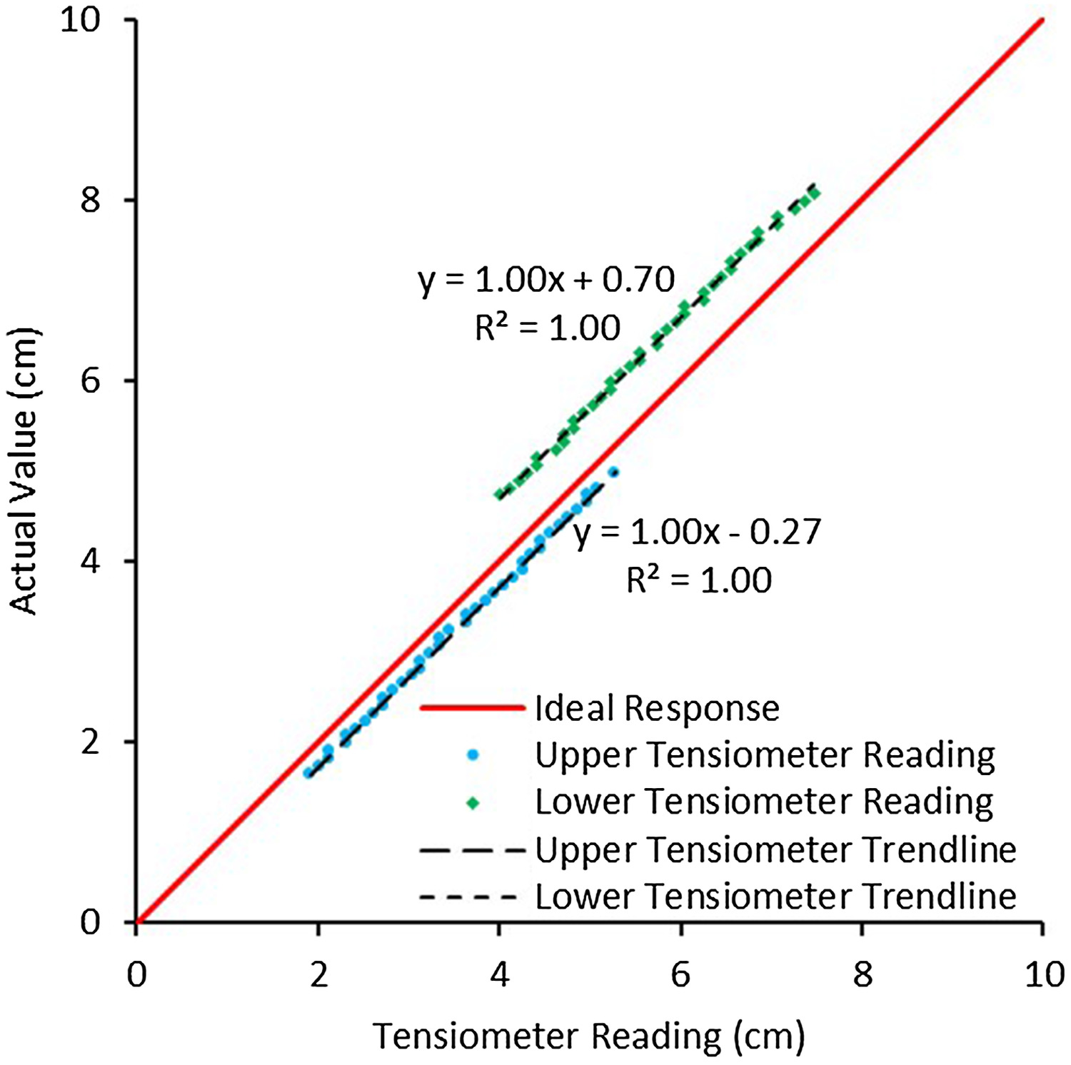
The net offset error (i.e., ) can be either negative or positive depending on the values and signs of and . For the results in Fig. 4, we obtained a net-negative offset error of for our system. In this study, we discuss issues related to both net-positive and net-negative offsets because they lead to different outcomes, yielding either under- or overestimation of UHC data, as discussed in the following section.
Implications of Tensiometer Offset Error and Analysis of UHC Data
To illustrate all possible implications of tensiometer offset errors, we processed the Experiment 1 data set to generate two additional data sets to account for net-negative and net-positive offset errors. Because our system had a net-negative offset error of , we simply used our observed data points without the tensiometer correction to assemble the net-negative offset error data set. To illustrate the effects of a net-positive offset error, we created an additional data set by reversing the direction of both offset errors (i.e., and ). This resulted in a net-positive offset error of 0.97 cm, allowing us to assemble a net-positive offset error data set.
Fig. 5 compares the UHC functions (i.e., estimated UHC values plotted as a function of matric potential) evaluated using net-positive and net-negative offset error data sets against the function for the fully corrected baseline experimental data. The corrected data set yielded more-realistic values in the wet range. The UHC function obtained from the corrected data approached the independently measured saturated hydraulic conductivity value of (a mean value of with a standard deviation of was measured using the falling head method, and these estimates are shown in the figure using an error bar). Conversely, the net-negative offset error data set resulted in an overestimating trend [similar to that in Fig. 1(a)], whereas the net-positive offset error data set caused an underestimating trend [similar to that in Fig. 1(b)]. We discuss these trends in the following section.
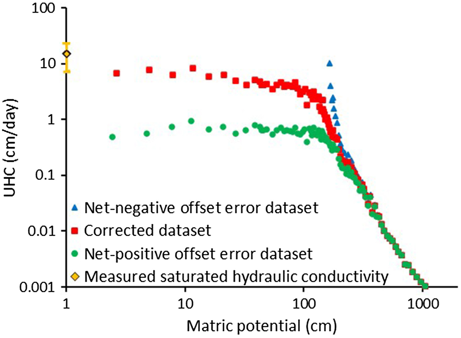
To explain these UHC data further and to fully understand their implications, we prepared two additional figures that summarize the results of the various intermediate calculations used to compute the UHC values. Fig. 6(a) presents the temporal changes in hydraulic gradient values, whereas Fig. 6(b) presents the corresponding temporal changes in UHC values. To understand the over- or underestimation trends in Fig. 5, we first review the hydraulic gradient values estimated for the corrected data set [Fig. 6(a), square symbols]. The corrected data points followed the expected trend, in which the gradient starts at zero and then increases as the sample dries. This should be expected because we initiated the system under hydrostatic conditions and then dried the soil by evaporating the water from the top surface. Furthermore, the smoothed trend of corrected data points also depicts a decrease in UHC values as the sample dried [Fig. 6(b)]. The UHC values estimated near the wet range (at early times) were close to the independently measured value for the saturated hydraulic conductivity, and indicate an overall decrease to lower values with time, despite the short-term noisy fluctuations in the data.
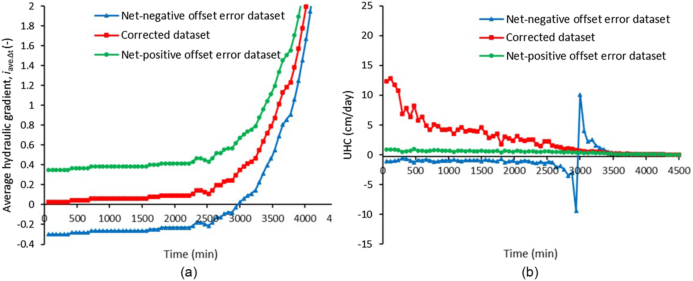
Unlike the corrected data set, the net-negative offset error data set (Fig. 5, triangle symbols) had an unrealistic overestimation trend that was almost identical to the spurious trend observed in some UHC functions in the literature data [Fig. 1(a), hollow circles]. This overestimation trend originated from the inaccuracies in the hydraulic gradient calculations, which can be inferred from the data in Fig. 6(a). The hydraulic gradient values for the net-negative offset error data set [Fig. 6(a), triangle symbols] yielded negative hydraulic gradient values during the initial drying period [for about 2 days (3,000 mins)]. These negative values are unrealistic because we initiated the system under hydrostatic conditions, and hence the starting gradient should have been zero, not a negative value. In turn, Fig. 6(b) (triangle symbols) illustrates how these incorrect negative hydraulic gradient values impacted UHC calculations. The UHC data [computed using Eq. (1)] also yielded unrealistic negative values until 3,000 mins. At about 3,000 min, the data had spurious oscillations in which the UHC values swung from extreme negative values to extreme positive values. This oscillation region corresponds to the period in which the estimated hydraulic gradient values gradually transition from negative to positive values [Fig. 6(a)]. During this period, the computed values of hydraulic gradient first become extremely small and negative (almost close to zero); and subsequently, after crossing the zero point, they become extremely small but positive; this leads to the undershoot and subsequent overshoot observed in UHC data. The value of the matric potential measured at the zero-crossing point (about 3,000 min) was about 160 cm, and the under- and overshoot effects are evident in Fig. 5 at about 160 cm of matric potential. Typically, in the published literature, researchers used a log-scale graph to present the UHC functions; because these graphs ignore negative data, they cannot display the oscillation in the negative direction. However, the oscillation in the positive direction (upward overshoot trend) is evident in some published data sets [e.g., Fig. 1(b)]. Of course, all these incorrect data points often are ignored, and are dealt with simply by invoking arbitrary rejection criteria (Peters and Durner 2008). In this study, for the first time, we clearly illustrate this spurious oscillation problem by carefully analyzing a measured data set with a net-negative offset error.
The circle symbols in Figs. 5 and 6(a and b) illustrate the implications of a net-positive offset error, which results in a systematic underestimation of the UHC values in the wet range. Interestingly, there were no oscillations in the net-positive offset error case, because the hydraulic gradient values were consistently positive from the beginning [Fig. 6(a), circle symbols]. However, these initial positive hydraulic gradient values are unrealistic because we started the experiment under hydrostatic conditions. Fig. 6(b) (circle symbols) illustrates how these incorrect positive hydraulic gradient values yield lower UHC values that are nearly an order of magnitude less than the expected corrected values.
Reproducibility of UHC and SWR Data with the Proposed Protocol
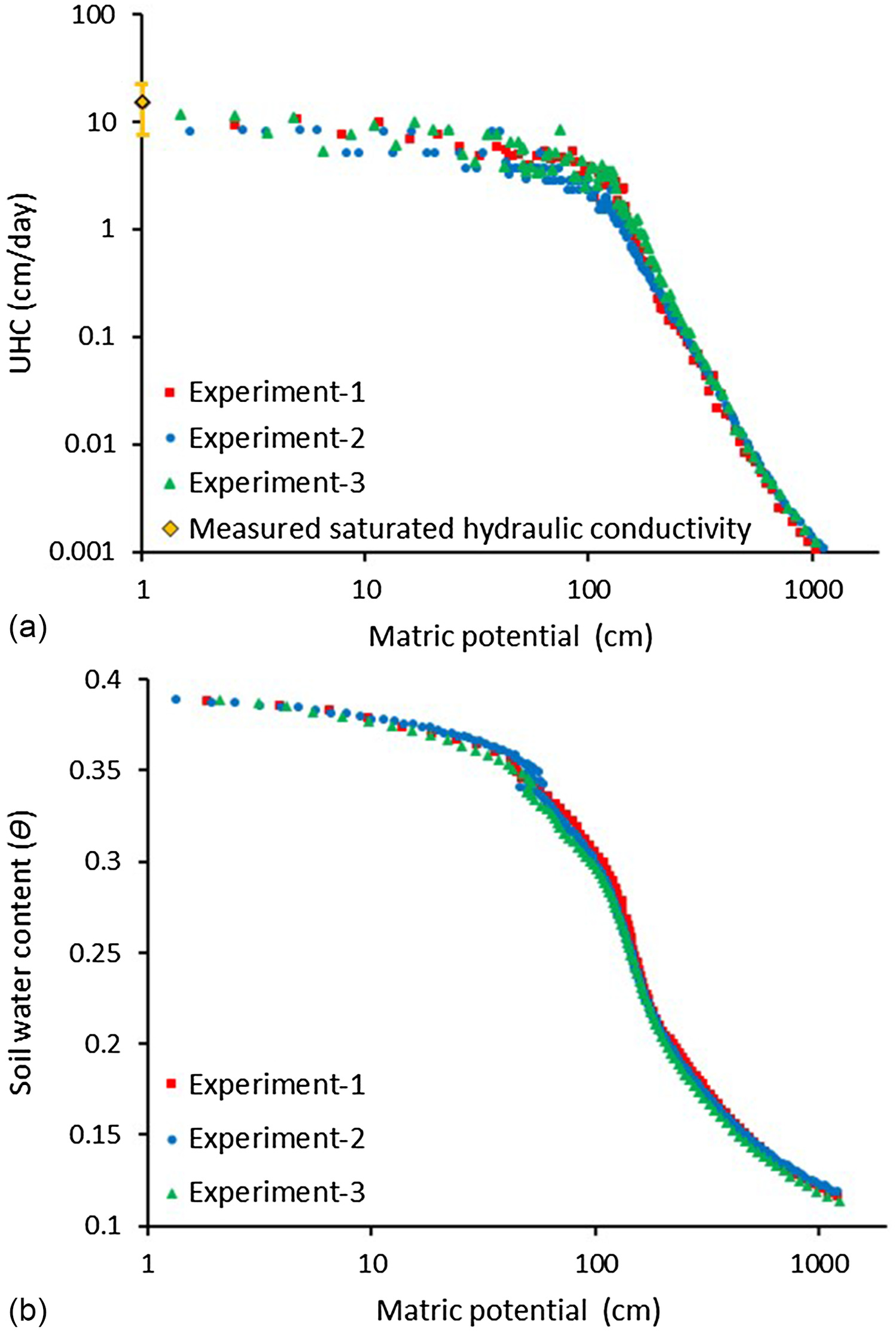
The previous section demonstrated how various over- or underestimation problems in UHC data (Fig. 1) can be resolved by using the proposed experimental protocol. However, the literature data also show issues with the reproducibility of SWR data (Fig. 2). To illustrate the robustness of the proposed experimental protocol in yielding stable and reproducible UHC and SWR data sets, we compared the results of the three independent experiments (i.e., different samples prepared using the same soil) completed with the proposed experimental procedure. Figs. 7(a and b) compare the UHC and SWR data collected from Experiments 1, 2, and 3, all of which used the proposed tensiometer-correction and sample-saturation procedures. These data show that the proposed protocol greatly improves SWR reproducibility; all three data sets are almost identical. Unlike the literature case (Fig. 2), which had considerable variability near the wet range due to incomplete saturation, the variations in the SWR data sets in Fig. 7(b) are almost negligible. The UHC data did have some natural random variability, but these were of the same order of magnitude as that observed in the measured values of saturated hydraulic conductivity.
Summary and Conclusions
The EV method is one of the most popular methods for developing UHC and SWR functions. However, the method’s accuracy near saturated conditions (i.e., in the wet range) has always been poor. Therefore, researchers often have used different types of rejection criteria to discard the wet-range data obtained using the EV method (e.g., Peters and Durner 2008). This practice can result in discarding important data points collected near the wet region. In this study, we present experimental evidence that demonstrates how variabilities in UHC and SWR data collected near the wet range originate from the errors associated with tensiometer calibration and sample saturation procedures. Our data show that even a relatively minor tensiometer offset error, on the order of variation in the measured matric potential values, can result in an order of magnitude error in the UHC estimates. To address these problems, we propose a practical experimental protocol that includes a tensiometer calibration method completed directly on the test sample, and a robust sample saturation procedure. Our results show that the proposed calibration procedure effectively quantifies the offset error, and that accounting for this error significantly reduces both over- and underestimation errors in UHC data collected at the wet range. We tested the robustness of the proposed protocol by repeating the experiment three times to quantify its reproducibility. The results show that the proposed protocol generates more-reliable and -stable UHC and SWR data in the wet range. Our study contributes to a deeper understanding of the performance of the EV method in the wet range, and uses this new knowledge to enhance the overall reliability of the method for characterizing unsaturated soil properties.
Data Availability Statement
All the data are provided in the figures. The data sets used for generating these figures are available from the corresponding author upon reasonable request.
Acknowledgments
The authors thank the three anonymous reviewers for their constructive comments and suggestions. Funding for this project was provided in part by a Cooperative Institute for Research to Operations in Hydrology (CIROH) grant awarded through the NOAA’s Cooperative Agreement with the University of Alabama, NA22NWS4320003; and National Science Foundation Grant OIA 2019561. The authors also thank Sama Memari and Mahlet Kebede for conducting various preliminary evaporation experiments.
Author contributions: Nam and Clement jointly developed the ideas; Nam and Poudyal conducted the experiments; Nam and Poudyal prepared the figures; Nam, Clement, and Srinivasan jointly wrote and revised the manuscript; and Clement supervised the work and developed the funding support and laboratory facilities. All four authors have read and approved the final manuscript.
References
Ahuja, L. R., K. E. Johnsen, and G. C. Heathman. 1995. “Macropore transport of a surface-applied bromide tracer: Model evaluation and refinement.” Soil Sci. Soc. Am. J. 59 (5): 1234–1241. https://doi.org/10.2136/sssaj1995.03615995005900050004x.
Bezerra-Coelho, C. R., L. Zhuang, M. C. Barbosa, M. A. Soto, and M. T. van Genuchten. 2018. “Further tests of the HYPROP evaporation method for estimating the unsaturated soil hydraulic properties.” J. Hydrol. Hydromech. 66 (2): 161–169. https://doi.org/10.1515/johh-2017-0046.
Boels, D., J. B. H. M. van Gils, G. J. Veerman, and K. E. Wit. 1978. “Theory and system of automatic determination of soil moisture characteristics and unsaturated hydraulic conductivities.” Soil Sci. 126 (4): 191–199.
Breitmeyer, R. J., and L. Fissel. 2017. “Uncertainty of soil water characteristic curve measurements using an automated evaporation technique.” Vadose Zone J. 16 (13): 1–11. https://doi.org/10.2136/vzj2017.07.0136.
Fujimaki, H., and M. Inoue. 2003. “A transient evaporation method for determining soil hydraulic properties at low pressure.” Vadose Zone J. 2 (3): 400–408. https://doi.org/10.2113/2.3.400.
Henseler, K. L., and M. Renger. 1969. “Die Bestimmung der Wasserdurchlässigkeit im wasserungesättigten Boden mit der Doppelmembran-Druckapparatur.” Z. Pflanzenernahr. Bodenkd. 122 (3): 220–228. https://doi.org/10.1002/jpln.19691220304.
Inforsato, L., S. Iden, W. Durner, A. Peters, and Q. De Jong van Lier. 2023. “Improved calculation of soil hydraulic conductivity with the simplified evaporation method.” Vadose Zone J. 22 (5): e20267. https://doi.org/10.1002/vzj2.20267.
Kaluarachchi, J. J., and J. C. Parker. 1987. “Effects of hysteresis with air entrapment on water flow in the unsaturated zone.” Water Resour. Res. 23 (10): 1967–1976. https://doi.org/10.1029/WR023i010p01967.
Klute, A. 1972. “The determination of the hydraulic conductivity and diffusivity of unsaturated soils.” Soil Sci. 113 (4): 264–276.
Liu, Q., P. Xi, J. Miao, and X. Cao. 2021. “An alternative simplified evaporation method for measuring the hydraulic conductivity function of the unsaturated soils.” Eurasian Soil Sci. 54 (Dec): 1359–1366. https://doi.org/10.1134/S1064229321090052.
Machaček, J., W. Fuentes, P. Staubach, H. Zachert, T. Wichtmann, and T. Triantafyllidis. 2023. “A theory of porous media for unsaturated soils with immobile air.” Comput. Geotech. 157 (May): 105324. https://doi.org/10.1016/j.compgeo.2023.105324.
Masaoka, N., and K. I. Kosugi. 2018. “Improved evaporation method for the measurement of the hydraulic conductivity of unsaturated soil in the wet range.” J. Hydrol. 563 (Aug): 242–250. https://doi.org/10.1016/j.jhydrol.2018.06.005.
Minasny, B., and D. J. Field. 2005. “Estimating soil hydraulic properties and their uncertainty: The use of stochastic simulation in the inverse modelling of the evaporation method.” Geoderma 126 (3–4): 277–290. https://doi.org/10.1016/j.geoderma.2004.09.015.
Mohrath, D., L. Bruckler, P. Bertuzzi, J. C. Gaudu, and M. Bourlet. 1997. “Error analysis of an evaporation method for determining hydrodynamic properties in unsaturated soil.” Soil Sci. Soc. Am. J. 61 (3): 725–735. https://doi.org/10.2136/sssaj1997.03615995006100030004x.
Peters, A., and W. Durner. 2008. “Simplified evaporation method for determining soil hydraulic properties.” J. Hydrol. 356 (1–2): 147–162. https://doi.org/10.1016/j.jhydrol.2008.04.016.
Peters, A., S. C. Iden, and W. Durner. 2015. “Revisiting the simplified evaporation method: Identification of hydraulic functions considering vapor, film and corner flow.” J. Hydrol. 527 (Aug): 531–542. https://doi.org/10.1016/j.jhydrol.2015.05.020.
Sakaguchi, A., T. Nishimura, and M. Kato. 2005. “The effect of entrapped air on the quasi-saturated soil hydraulic conductivity and comparison with the unsaturated hydraulic conductivity.” Vadose Zone J. 4 (1): 139–144. https://doi.org/10.2136/vzj2005.0139.
Schelle, H., S. C. Iden, and W. Durner. 2011. “Combined transient method for determining soil hydraulic properties in a wide pressure head range.” Soil Sci. Soc. Am. J. 75 (5): 1681–1693. https://doi.org/10.2136/sssaj2010.0374.
Schindler, U. 1980. “Ein schnellverfahren zur messung der wasserleitfähigkeit im teilgesättigten boden an stechzylinderproben.” Arch. Acker-u. Pflanzenbau u. Bodenkd. Berlin 24 (1): 1–7.
Schindler, U., W. Durner, G. von Unold, L. Mueller, and R. Wieland. 2010b. “The evaporation method: Extending the measurement range of soil hydraulic properties using the air-entry pressure of the ceramic cup.” J. Plant Nutr. Soil Sci. 173 (4): 563–572. https://doi.org/10.1002/jpln.200900201.
Schindler, U., W. Durner, G. von Unold, and L. Müller. 2010a. “Evaporation method for measuring unsaturated hydraulic properties of soils: Extending the measurement range.” Soil Sci. Soc. Am. J. 74 (4): 1071–1083. https://doi.org/10.2136/sssaj2008.0358.
Schindler, U., L. Mueller, M. da Veiga, Y. Zhang, S. Schlindwein, and C. Hu. 2012. “Comparison of water-retention functions obtained from the extended evaporation method and the standard methods sand/kaolin boxes and pressure plate extractor.” J. Plant Nutr. Soil Sci. 175 (4): 527–534. https://doi.org/10.1002/jpln.201100325.
Schindler, U., and L. Müller. 2006. “Simplifying the evaporation method for quantifying soil hydraulic properties.” J. Plant Nutr. Soil Sci. 169 (5): 623–629. https://doi.org/10.1002/jpln.200521895.
Stonestrom, D. A., and J. Rubin. 1989. “Water content dependence of trapped air in two soils.” Water Resour. Res. 25 (9): 1947–1958. https://doi.org/10.1029/WR025i009p01947.
Tamari, S., L. Bruckler, J. Halbertsma, and E. J. Chadoeuf. 1993. “A simple method for determining soil hydraulic properties in the laboratory.” Soil Sci. Soc. Am. J. 57 (3): 642–651. https://doi.org/10.2136/sssaj1993.03615995005700030003x.
van Genuchten, M. T. 1980. “A closed-form equation for predicting the hydraulic conductivity of unsaturated soils.” Soil Sci. Soc. Am. J. 44 (5): 892–898. https://doi.org/10.2136/sssaj1980.03615995004400050002x.
van Schaik, J., and G. E. Laliberte. 1969. “Soil hydraulic properties affected by saturation technique.” Can. J. Soil Sci. 49 (1): 95–102. https://doi.org/10.4141/cjss69-011.
Wendroth, O., W. Ehlers, J. W. Hopmans, H. Kage, J. Halbertsma, and J. H. M. Wösten. 1993. “Reevaluation of the evaporation method for determining hydraulic functions in unsaturated soils.” Soil Sci. Soc. Am. J. 57 (6): 1436–1443. https://doi.org/10.2136/sssaj1993.03615995005700060007x.
Wendroth, O., and J. Simunek. 1999 “Soil hydraulic properties determined from evaporation and tension infiltration experiments and their use for modeling field moisture status.” In Proc., Int. Workshop on Characterization and Measurement of the Hydraulic Properties of Unsaturated Porous Media, edited by M. T. H. van Genuchten, F. J. Leij, and L. Wu, 737–748. Los Angeles: Univ. of California.
Wind, G. P. 1968. “Capillary conductivity data estimated by a simple method.” In Proc., Wageningen Symp., edited by P. E. Rijtema and H. Wassink, 181–191. Oxfordshire, UK: International Association of Hydrological Sciences.
Information & Authors
Information
Published In

Journal of Hydrologic Engineering
Volume 29 • Issue 6 • December 2024
Copyright
This work is made available under the terms of the Creative Commons Attribution 4.0 International license, https://creativecommons.org/licenses/by/4.0/.
History
Received: Nov 27, 2023
Accepted: Jun 10, 2024
Published online: Aug 24, 2024
Published in print: Dec 1, 2024
Discussion open until: Jan 24, 2025
Authors
Metrics & Citations
Metrics
Citations
Download citation
If you have the appropriate software installed, you can download article citation data to the citation manager of your choice. Simply select your manager software from the list below and click Download.