Testing the Multivariate Hüsler–Reiss Model as a Practical Parametric Approach for Multiple River Flood Risk Assessment Using d4PDF Data: A Case Study in Kyushu Island, Japan
Publication: Journal of Hydrologic Engineering
Volume 29, Issue 3
Abstract
Compound flood disaster risks are increasing due to multiple river floods within a single storm event. Many studies targeted dependence structure based on multivariate extreme value theory; however, fewer studies focused on the sum of subset joint probabilities (SSJP), defined as the probability that any combination of rivers are flooded over the target area as an integral index of compound flooding risks. Modeling multivariate extremes at high dimensions faces two challenges: model complexity and sample size. In this study, as a classical asymptotic dependence model, the Hüsler–Reiss (HR) model was explored to resolve the former issue owing to its simplicity. From the multivariate HR model, any subset joint probability is explicitly obtained without numerical integration of angular measure, and dependence parameters are constructed from only pairwise parameters. The latter challenge was addressed using a large ensemble (50 members of 60-year simulation) of the database for policy decision-making for future climate change (d4PDF), which is consequently regarded as the annual maximum flow data of 3,000 years. This study analytically derived SSJP based on the HR model and tested its applicability using annual maximum flow data simulated from d4PDF for 20 rivers in Kyushu Island, Japan. The simulated SSJP based on the HR model and empirical SSJP were compared as the probability plot of the number of river basins where peak discharge exceeds the design level. As a result, under the constraint of HR that the partial correlation must range from to 1, the estimated SSJP by the HR model was in agreement with the empirical SSJP. The case study presents promising results of the proposed HR model–based approach.
Introduction
Due to a variety of hydrological extremes intensified in a changing climate, compound (multivariate) flooding events pose a serious threat across the globe. The escalating risk of compound flood is projected from a global scale (Zscheischler et al. 2018) to a national scale (Wahl et al. 2015) to a regional scale (Tanaka et al. 2020). Assessment of such multivariate extreme risks has been addressed using many multivariate models. In existing literature of water resources management, a number of dependence models have been applied and tested against multivariate data such as three variables (rainfall deficit, soil moisture deficit, and high temperature) for drought risk analysis (Sharma and Mujumdar 2022), high flow discharge of two tributary rivers (Neal et al. 2013), and two variables of compound flood risk factors (river flooding and storm surges) (Zellou and Rahali 2019). However, these studies targeted two or three variables due to the limitations of model flexibility and sample size (Kotz and Nadarajah 2000; Dey and Yan 2016). Some alternative approaches have been shown to overcome the former challenge. Heffernan and Tawn (2004) proposed a conditional approach to estimate the exceedance probability of multiple target variables as one exceeds a threshold. Owing to its flexibility, the nationwide assessment of concurrent flood risks in the United Kingdom (Keef et al. 2009), the European Union (Diederen et al. 2019), or the United States (Quinn et al. 2019) was implemented. Graphical models have also gained popularity for their flexibility in the dependence modeling of high-dimensional extremes (Engelke and Hitz 2020).
These approaches overcame the curse of dimensionality by avoiding from formulating multivariate extreme value distributions (MEVDs) in extremely high dimensions. On the other hand, from a family of MEVDs, a few practical models have been proposed and applied, trying to avoid the dimensional issues by constructing a model with fewer parameters. For example, Cooley et al. (2010) proposed a new construction of an angular density for the pairwise beta distribution, with only pairwise parameters and a global parameter (), and applied to spatial air quality data. They focused on the situation where threshold exceedance data were preferred over block maxima data. As introduced by Mostofi Zadeh et al. (2019), hydrological frequency analysis in practice prefers block maxima data because annual maximum data are a more commonly available form of data (Centre for Ecology and Hydrology 1999) and are away from the threshold selection issue (Solari and Losada 2012), which is also the case in the area of this study in Japan (Tanaka et al. 2002). However, such studies hardly show the explicit form of joint probabilities, which is more appropriate for multiple hazard risk assessment. Sharma and Mujumdar (2022) applied asymmetric logistic, Dirichlet, Hüsler–Reiss (HR), and pairwise beta models to meteorological and hydrological data (e.g., drought, monthly maximum temperature, rainfall deficit, and soil moisture deficit), showing that the HR model was flexible and outperformed the others in three-dimensional (3D) analysis. The HR model would be considered to take a central place of multivariate extreme value analysis, such as a multivariate normal distribution applied to general statistical problems, and moreover it is efficient, meaning that all the dependence parameters are obtained from the combination of pairwise parameters, while the target dimension is flexibly changeable, which are not satisfied in some popular models, such as the pairwise beta distribution (Husler and Reiss 1989). The graphical model proposed by Engelke and Hitz (2020) employs the HR model for building the dependence structure. The Heffernan and Tawn model is a conditional model, i.e., the aforementioned previous studies using this model calculated joint probability of all target locations in a certain region by multiplying conditional cumulative probability by the marginal cumulative probability of a single conditioned location as an origin. This framework avoids treating too many combinations. On the other hand, the multivariate HR model explicitly derives the whole function of multivariate cumulative probability, keeping simplicity by deriving dependence of all pairs from the bivariate HR model; therefore, this study explored the applicability of this model.
As a practical index of multiriver flood risk, instead of the joint probability of all rivers, this study examined the sum of subset joint probabilities (SSJP), defined as the probability that any combinations of rivers are flooded (exceeding such as 100-year design flow) over the target area (see the detail explanation and the formula of probability calculation in “Results”). For such a purpose, the parameter scalability in the HR model is useful because it can derive SSJP for various combinations only with pairwise parameters, while it is also a limitation in that, when any combination of pairwise parameters is inappropriate, the model cannot be constructed. Previous studies in related literature focused on the capability (flexibility or robustness) of spectral density (Boldi and Davison 2007; Engelke et al. 2015; Sharma and Mujumdar 2022). To demonstrate the aforementioned usefulness of the multivariate HR model more directly, this study estimated SSJP over a target region using the HR model.
In Japan, a heavy rainfall event during the Baiu (rainy) season in western Japan in 2018 and Typhoon Hagibis in 2019 caused multiple river flooding (MLIT 2018, b). However, such cases are rare in statistics, and thus hard to quantify as frequency based on observation data of river flow, which are available only for the past 30 years. The sample size issue has been addressed in the climate change research through an ensemble climate simulation approach. In parallel with the increased computing power and advanced climate sciences, several research institutes have successfully produced a large ensemble of climate simulation data. For example, in Japan, a database for policy decision-making for future climate change (d4PDF) has been jointly produced using the Earth Simulator, in coordination with various science programs [SOUSEI, TOUGOU, SI-CAT, and data integration analysis system (DIAS)] of the Ministry of Education, Culture, Sports, Science, and Technology (MEXT) (Mizuta et al. 2017). This data set has been widely used in impact assessment of extreme weather events, such as river flooding, wind disaster, and coastal flooding (Ishii and Mori 2020). Kobayashi et al. (2020) developed a distributed rainfall-runoff model (1K-DHM) (Tanaka and Tachikawa 2015) for 109 major river basins (classified as Class A in terms of societal and economic importance by the Japanese government) and simulated annual maximum river discharges from d4PDF rainfall data with bias correction over Japan, which generated thousands of years of extreme river discharge data for periods of interest. Fully utilizing this large-ensemble, bias-corrected data set, this study aimed to overcome the sample size issue and clarify the asymptotic probability of simultaneously occurring flooding events of rivers among rivers. Tanaka et al. (2021) investigated a number of rivers with river discharges at the reference stations exceeding the design level, simulated river discharges from d4PDF rainfall data, and discussed geographical features via association rule analysis and graph theory. However, they neither analyzed asymptotic dependence nor discussed robustness of obtained dependence structure. Tanaka and Kitano (2022) analyzed the asymptotic dependence structure between two river basins using d4PDF, confirming that typical decadal record length is not enough to robustly identify tail dependency. On the other hand, its extension to multiple dimensions more than two including deriving SSJP has not been addressed yet.
The objective of this study was to propose a framework for estimating the multivariate probability of the number of flooded rivers (i.e., river discharge at the reference station exceeding the threshold return period) by deriving SSJP based on the HR model. Then, its applicability was tested in a case study in Japan using a large-ensemble river discharge data set of d4PDF. The country has been heavily damaged repeatedly. A heavy rainfall event during the Baiu season in western Japan in 2018 caused flooding in eight major rivers and resulted in 237 casualties, while Typhoon Hagibis in 2019 caused about 58 billion yen of insurance loss (MLIT 2018, 2019). In particular, we selected Kyushu Island where both severe rain bands in the Baiu season and typhoons often attack. “Data and Study Area” describes a large-ensemble climate simulation data set d4PDF and the study area. “Methods” introduces the methods starting with bivariate and multivariate HR model in “Bivariate Extreme Value Theory” and “Multivariate Hüsler–Reiss Model,” respectively, followed by the derivation of SSJP from various dimensional HR model “Developing the SSJP Model” and the simulation workflow in “Methodological Steps to Derive SSJP Based on Multivariate Hüsler–Reiss Model.” “Results” shows the fitting result of the SSJP with the HR model starting with a generalized extreme value distribution as a marginal distribution in “Performance of the Univariate Extreme Value Distribution,” bivariate dependence estimations and SSJP in “Two-River-Flood Probability” and the validation of derived SSJP in “Validation for Multiple River Flood Probability.” The characteristics of the obtained parameters and the applicability (limitations) of the framework are discussed in “Discussions.” Finally, “Conclusions” summarizes the discussions and limitations.
Data and Study Area
The data set of d4PDF was developed by a large ensemble of simulations of the past and future global climate (Mizuta et al. 2017) with the global climate model (AGCM-3.2S) at a spatial resolution of 60 km and downscaled with the 20-km nonhydrostatic regional climate model (NHRCM) (Sasaki et al. 2008) for Japan. The dynamically downscaled data in the past climate experiment contain 60-year climate simulations from 1951 to 2010 with 50 ensembles, amounting to 3,000 simulation years in total. As mentioned, observed river flow data in Japan are assumed to lack for multivariate extreme value analysis. Therefore, this study collected all ensembles of d4PDF for testing the multivariate HR model. Kobayashi et al. (2020) identified the annual maximum rainfall event in each year for 109 Class A river basins in terms of -hour basin-average accumulation rainfall (BAAR), where is the design rainfall duration. They corrected model bias in BAAR from the observed BAAR using a quantile mapping method and simulated peak discharge from the bias-corrected rainfall data (defined as annual maximum floods) with a distributed rainfall-runoff model (1K-DHM) (Tanaka and Tachikawa 2015) for 109 major (named as Class A) river basins in Japan. As a result, the estimated design flow (corresponding to 100, 150, or 200 years in each basin) as the corresponding quantile from the simulated 3,000-year discharge was in a good agreement with actual design flow discharge set by the government [Fig. 10 in Kobayashi et al. (2020)]. This study employed the same 3,000-year data of simulated discharge in the past experiment in river basins in southern Japan and fit the MEVD framework to be described subsequently. This treatment was justified because the ensembles of boundary conditions of sea surface temperature and sea ice were all based on the observed data from COBE-SST2, and added perturbation was small compared with the observed value itself.
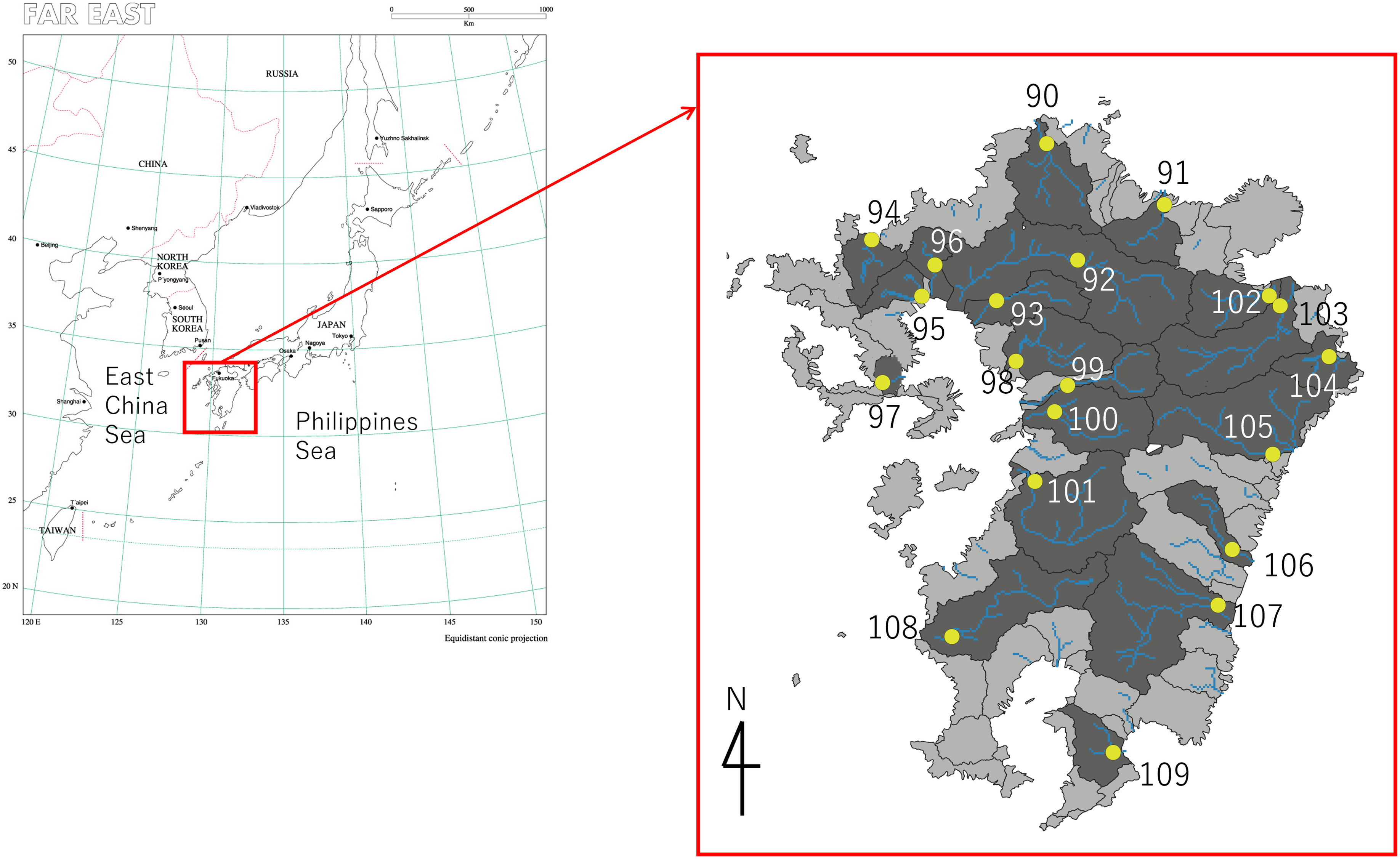
Simultaneous flood risks were investigated for 20 Class A river basins over the Kyushu region in Japan (Fig. 1). The hydrological summary of the target river basins is given in Table 1. The Kyushu region is an island isolated from the mainland of Japan. The island is composed of relatively small catchments (from 87 to ) and often experiences heavy rainfall. In particular, the west side is heavily affected by seasonal frontal rain during May–July (known as Baiu), while the east side receives huge rainfall by typhoons during August–October. Since 2010, heavy rainfall events have caused serious flood disasters frequently, especially in the west side by frontal rain events (2012, 2017, 2018). Therefore, high dependence among these river basins is expected in Kyushu Island.
| River | Name | Catchment area () | Design rainfall duration (h) |
|---|---|---|---|
| 90 | Onga | 1,026 | 48 |
| 91 | Yamakuni | 540 | 48 |
| 92 | Chikugo | 2,860 | 48 |
| 93 | Yabe | 647 | 9 |
| 94 | Matsuura | 446 | 48 |
| 95 | Rokkaku | 341 | 6 |
| 96 | Kase | 368 | 48 |
| 97 | Honmyo | 87 | 24 |
| 98 | Kikuchi | 996 | 12 |
| 99 | Shira | 480 | 48 |
| 100 | Midori | 1,100 | 12 |
| 101 | Kuma | 1,880 | 12 |
| 102 | Oita | 650 | 48 |
| 103 | Ono | 1,465 | 48 |
| 104 | Banjo | 464 | 12 |
| 105 | Gokase | 1,820 | 12 |
| 106 | Omaru | 474 | 9 |
| 107 | Oyodo | 2,230 | 48 |
| 108 | Sendai | 1,600 | 48 |
| 109 | Kimotsuki | 485 | 48 |
Note: Design rainfall duration is determined by the MLIT (2023).
Methods
Bivariate Extreme Value Theory
Let () be component-wise maxima. Using their random variable (), denote aswhere = cumulative distribution function (CDF) of the general extreme value (GEV) distribution of (); and is its location, scale, and shape parameters. From the Poisson process, one can easily derive that is the inverse of occurrence ratio and is interpreted as a return period of (). Then their bivariate extreme value distributions are given as follows:where = exponent measure. The occurrence probability of each extreme value exceeding a threshold (in a single event) is expressed as . Similarly, the occurrence ratio that either of the pair exceeds the threshold (which can be determined by ) is given as follows:
(1)
(2)
(3)
The inclusion-exclusion formula provides the co-occurrence ratio of both of the pair exceeding a threshold (which can be also determined by ) as follows:
(4)
The flood coincidence rate can be obtained through the dependence function included in the bivariate extreme value distributions of component-wise maxima.
In the bivariate case, the following index for measuring dependence is typically used. Setting the same threshold rate for both extreme values, i.e., considering the same risk level in both dimensions, and considering that the exponent measure satisfies the homogeneity of order of , that iswhere , the ratio of the co-occurrence rate to , can be described by the dependence function as follows:which is a constant value over the thresholds. Thus, is an important index for validating the convergence of data to MEVDs. Denoting the number of events when exceeds the threshold as , their correlation coefficient is derived as follows:
(5)
(6)
(7)
Therefore, hereinafter is called the correlation coefficient of occurrence ratio of extreme events. This correlation coefficient is not used in constructing multivariate models in this study but is calculated for discussing the characteristics of obtained dependence parameters for many combinations of bivariate models, because as described subsequently, the dependence parameters of the multivariate HR model are composed of the combinations of parameters in bivariate HR model.
Multivariate Hüsler–Reiss Model
The most important challenge of multivariate analysis may be the combinatorial explosion of dependence parameters. This study employed the multivariate HR model because all parameters of this model were constructed from bivariate dependence so the model could avoid the parameter combination explosion. The bivariate HR distribution function was as follows:where = CDF of the standardized normal distribution; and is a dependence parameter. As approaches zero and infinity, the model shows complete dependence and independence, respectively. For three dimensions, the exponent measure of the HR model is constructed not only by adding the third term to the two terms in the exponent of the bivariate model, but also by taking into account the mutual dependencies in each component formed by the normal distribution in the following:where = cumulative probability of the normal distribution with correlation . The correlation matrix of the two-dimensional normal distribution is given by
(8)
(9)
(10)
Finally, the HR model is generalized to dimensions by the following expressions:where ; ; and dimensional normal distribution with a correlation matrix . For all , the partial correlations in are .
(11)
(12)
As stated previously, the merit of this model was that the parameters were only dependences between two variables whose number only amounts to
In exchange for this advantage, the complexity of dependence structure was limited in that all elements of partial correlation must satisfy , i.e., the HR model is not constructed when the combination of does not satisfy the constraint of . It may be possible to fit the multivariate HR model to all dimensions at once and obtain optimal parameters under this constraint; however, this is dangerous in that the fitted model can be possibly selected as a local optimum solution over the likelihood space. This study tested the applicability of the proposed HR model from a viewpoint of modeled combinations.
Developing the SSJP Model
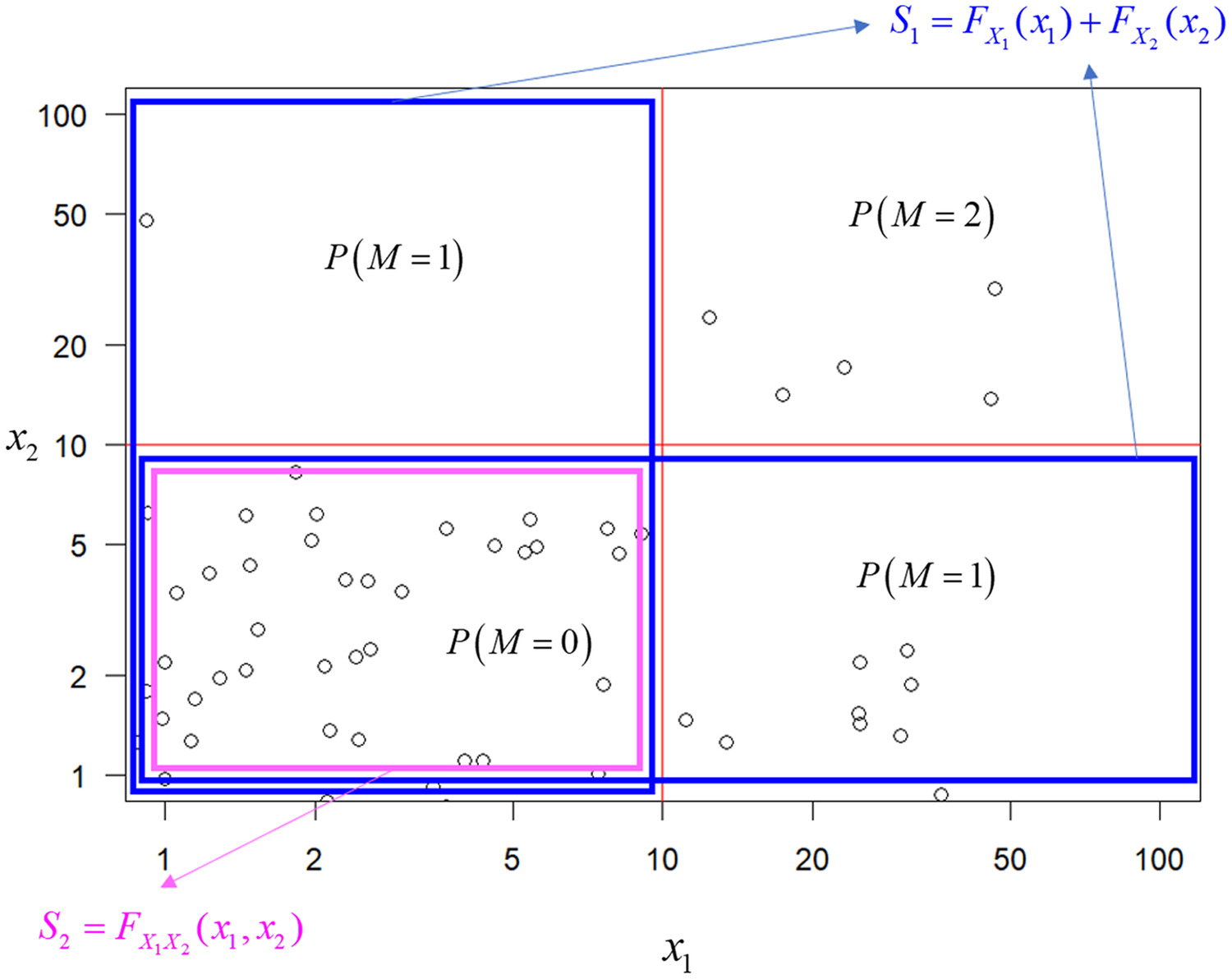
Once the multivariate model was identified, this study newly derived SSJP: the probability that the number of rivers exceeding their threshold return period becomes , as follows. Let us see an example of the two-dimensional (2D) and 3D cases. Denote as the threshold return period in the 2D case. The 2D domain is shown in Fig. 2. The probability of no flooding, i.e., , is simply obtained by the CDF itself . From the inclusion-exclusion formula, the probability that flooding occurs in one river is obtained as . The first two terms include the probability that flood level is below the threshold in each river, permitting duplication; then the duplication is removed by the final term. In the same way, the two-river-flooding probability is obtained as . In the 3D case, denoting as the threshold return period, each probability is obtained as follows:where ; ; and .
(13)
In general, the probability of rivers flooding can be derived from the combination theory (Feller 1957) as follows:for any dimensions, where is the sum of cumulative probabilities among all combinations of -dimensional HR models in dimensions and . It is also possible to construct this probability by the combination of occurrence ratio as demonstrated in the 2D case in Eq. (4). In this case, various occurrence ratios of concurrent threshold exceedance need to be combined appropriately. Because the smaller number of rivers flooded has higher occurrence probability, this study constructed the number of rivers flooded from concurrent nonexceedance of a threshold as shown in Eqs. (13) and (14).
(14)
Similarly, the cumulative probability of the number of flooded rivers is obtained as follows:
(15)
Finally, SSJP is derived as the probability that at least rivers are flooded
(16)
The indicator starts from and the subscript of is shifted to .
Methodological Steps to Derive SSJP Based on Multivariate Hüsler–Reiss Model
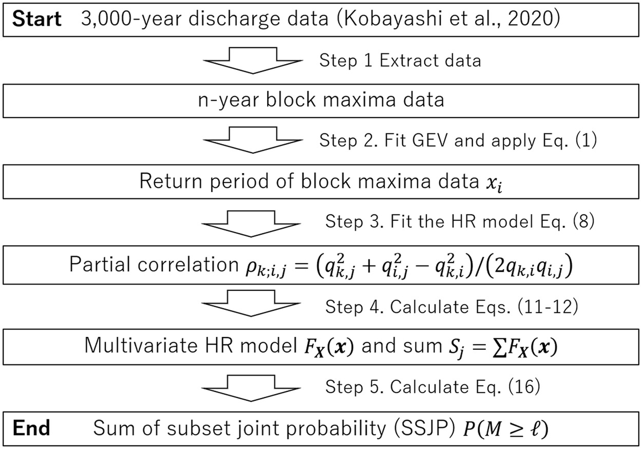
The preceding probability is calculated from the following steps:
Step 1. Extract -year block maxima data with a certain block size from 3,000-year annual maximum river discharge data.
Step 2. Fit the GEV distribution to the extracted block maxima data using the maximum likelihood method and convert the data to return period from Eq. (1).
Step 3. Fit the two-dimensional HR model Eq. (8) to all combinations of the component-wise maxima of converted return periods and calculate partial correlation from the fitted dependence parameter .
Step 4. Construct the multivariate HR model Eqs. (11) and (12) and derive the sum of CDF for all dimensions if all partial correlations satisfy .
Step 5. Calculate SSJP with Eq. (16).
See Fig. 3 for the graphical representation of the process. After Step 5, SSJP for one combination of river basins is obtained.
The confidence interval (CI) of the derived SSJP is explored by a bootstrap method. The most straightforward approach is a repetition of Steps 1–5, resampling a sample of 3,000 data points allowing the duplication from the original 3,000-year annual maximum river discharge data. All partial correlations in the multivariate HR model must satisfy for each resampled data. Therefore, the feasibility of CI based on bootstrap is also discussed subsequently in terms of the number of samples satisfying the condition. Because this approach for confidence interval is hard to implement as shown in the following results, for uncertainty evaluation, empirical SSJP in a nonparametric approach without fitting the HR model was conducted by counting up the number of river basins where the return period of the simulated discharge is beyond the threshold return period in the same year and evaluating the empirical cumulative probabilities. The “Results” section compares the derived SSJP in the proposed framework through Steps 1–5 and the empirical one through the aforementioned procedures. Empirical SSJP is also subject to sampling bias; therefore, the bootstrap method was applied again to derive its CI.
Results
The performance of the constructed model was tested against the d4PDF data (annual maximum river discharges). Making the best use of d4PDF with large ensembles (3,000 annual maximum data), various block sizes were tested. First, the convergence of univariate extreme values to GEV was explored. The river discharges in all combinations of two river basins were modeled by the bivariate HR model, which was validated in terms of the CDF of the angular component. Using the estimated dependence parameters, multivariate HR models and the resulting SSJP among multiple river floods were estimated and compared with the empirical CDF of SSJP obtained from the d4PDF data. In all analyses, R package evd (Stephenson 2002) was used. Parameters were fitted with the maximum likelihood method.
Performance of the Univariate Extreme Value Distribution
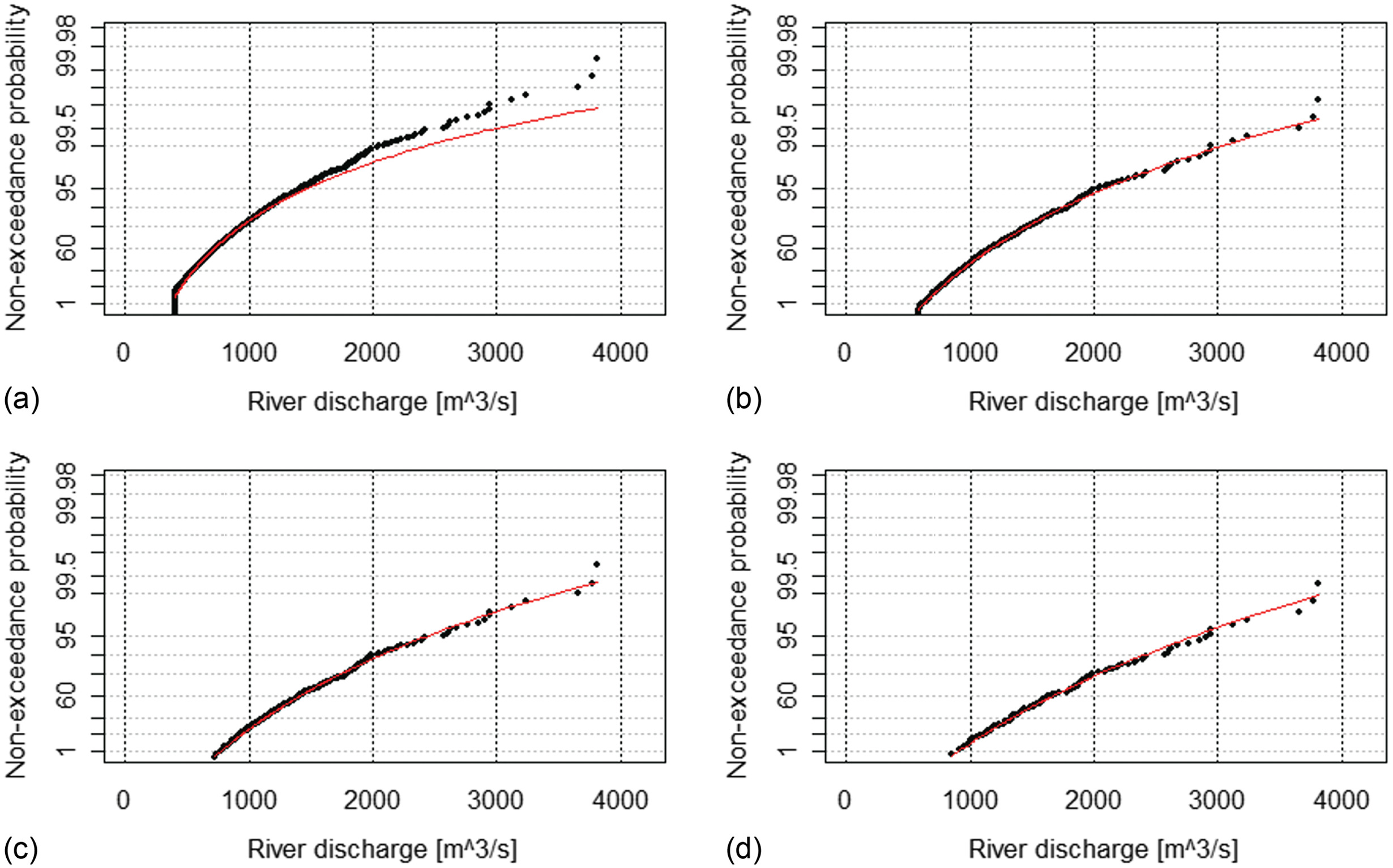
The GEV distribution was fitted to annual maximum river discharge data in 20 river basins. An example of River 95 (the Rokkaku River basin) is shown in Fig. 4. To see the asymptotic feature of the data, the block sizes of 1, 5, 10, 20, 40, 50, and 100 years were examined. The data better fit the GEV distribution as the block size became longer. This tendency was also reported by Tanaka and Kitano (2021) when testing other river basins. From both this study and the previous study, the block size as well as sample size, except for the sensitivity test of block sizes, was fixed to 20 years to ensure the convergence of data to extreme value theory.
Two-River-Flood Probability
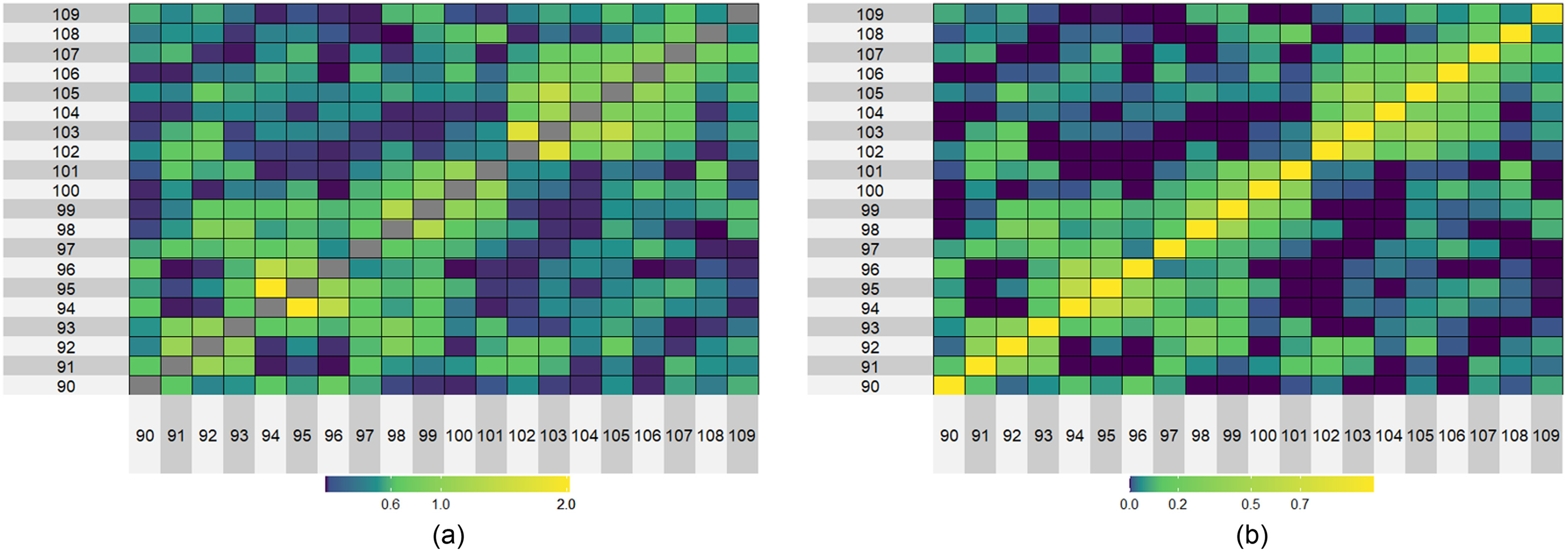
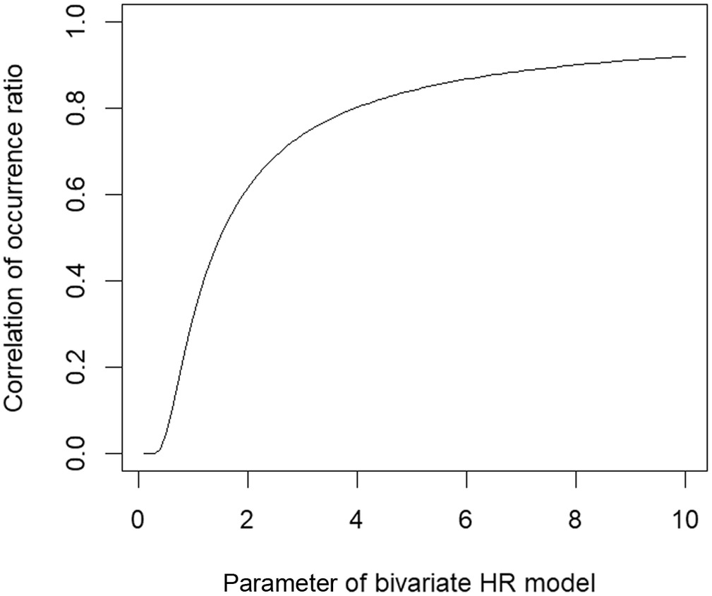
The estimated parameters and the correlation coefficient of occurrence ratio [Eq. (6)] are shown for 20 river basins in Fig. 5. The parameter of bivariate HR models [Fig. 5(a)] is drawn as for easier visibility. As the parameter became higher, the correlation increases (Fig. 6); therefore, Figs. 5(a and b) look similar. As expected, adjacent rivers (near the diagonal elements), which have a similar number, were highly correlated [lighter colors in Fig. 5(b)]. As a result, the figure suggests that there are two major groups composed of mutually correlated rivers: Rivers 90 to 101 and 102 to 109. As shown in Fig. 1, the former group faced the East China Sea, while the latter was on the Philippines Sea. A similar classification was stated by Tanaka et al. (2021), who used the same d4PDF river discharge data and employed the association rule analysis combined with graph theory, which justified the result in Fig. 5.
Validation for Multiple River Flood Probability
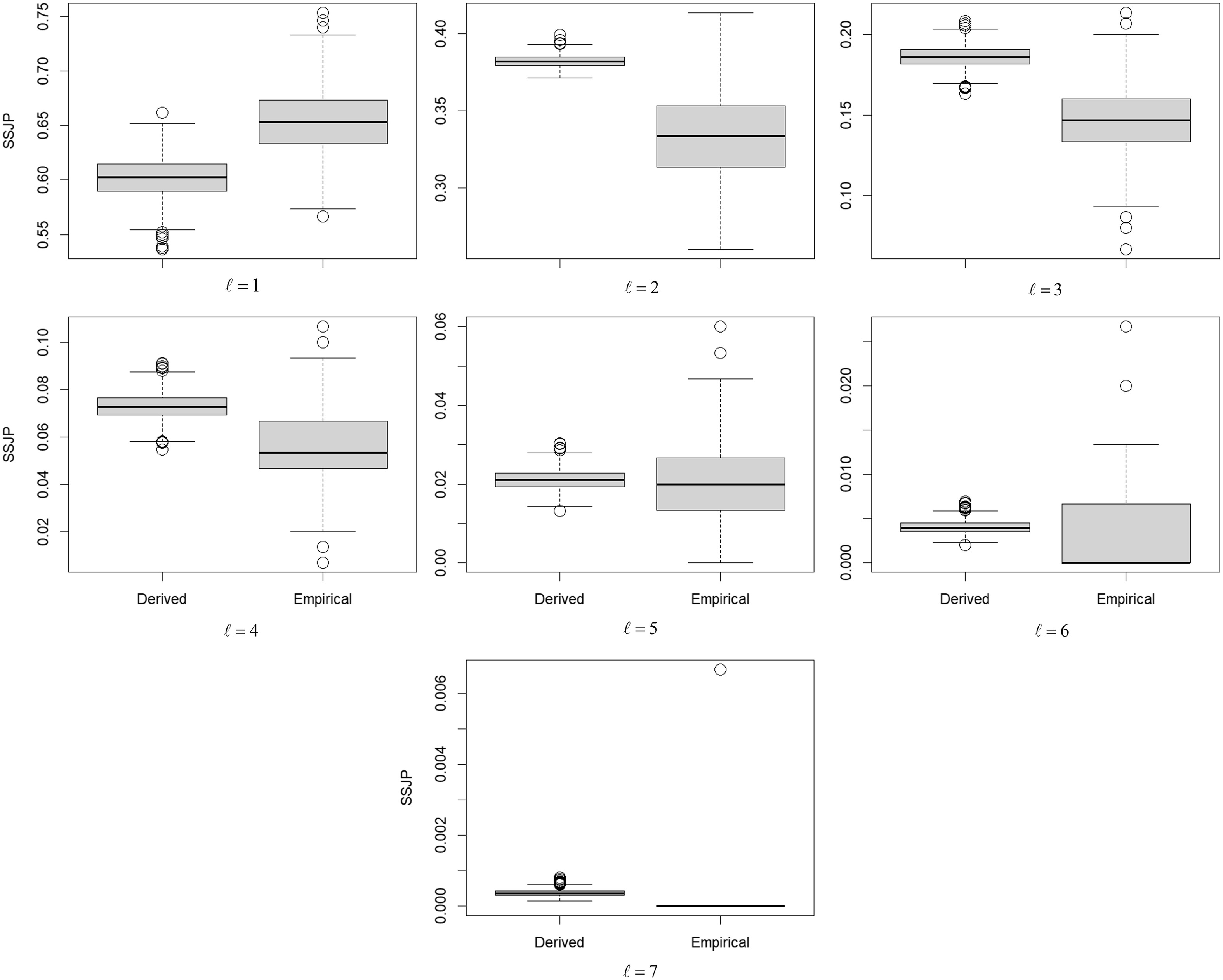
Among the 20 river basins, the proposed framework was applicable, i.e., all partial correlations in each subdimensional HR model satisfy , to some combinations of two to seven river basins. The number of combinations in which the multivariate HR model was constructable from bivariate HR models is given in Table 2. As examples, six (three) combinations of SSJP for river basins of size three (seven) is shown in Figs. 7 and 8. The threshold return period impact was explored for 100, 200, 500, and 1,000 years. Overall, the estimated exceedance probabilities based on the HR model (dashed lines) well corresponded to a nonparametric approach (circles), simply counting the number of flooded rivers (where peak discharge was over the threshold) from the d4PDF data for all cases. Other sizes of river basin (two, four, five, and six) showed similar results, indicating that the frequency of the number of flooded rivers is well represented by the HR model.
| Number of river basins, | Total number of combinations among all 20 river basins () | Constructable number of combinations for which all subdimensional HR models satisfy |
|---|---|---|
| 3 | 1,140 | 575 |
| 4 | 4,845 | 656 |
| 5 | 15,504 | 362 |
| 6 | 38,760 | 97 |
| 7 | 77,520 | 10 |
| — | 0 |
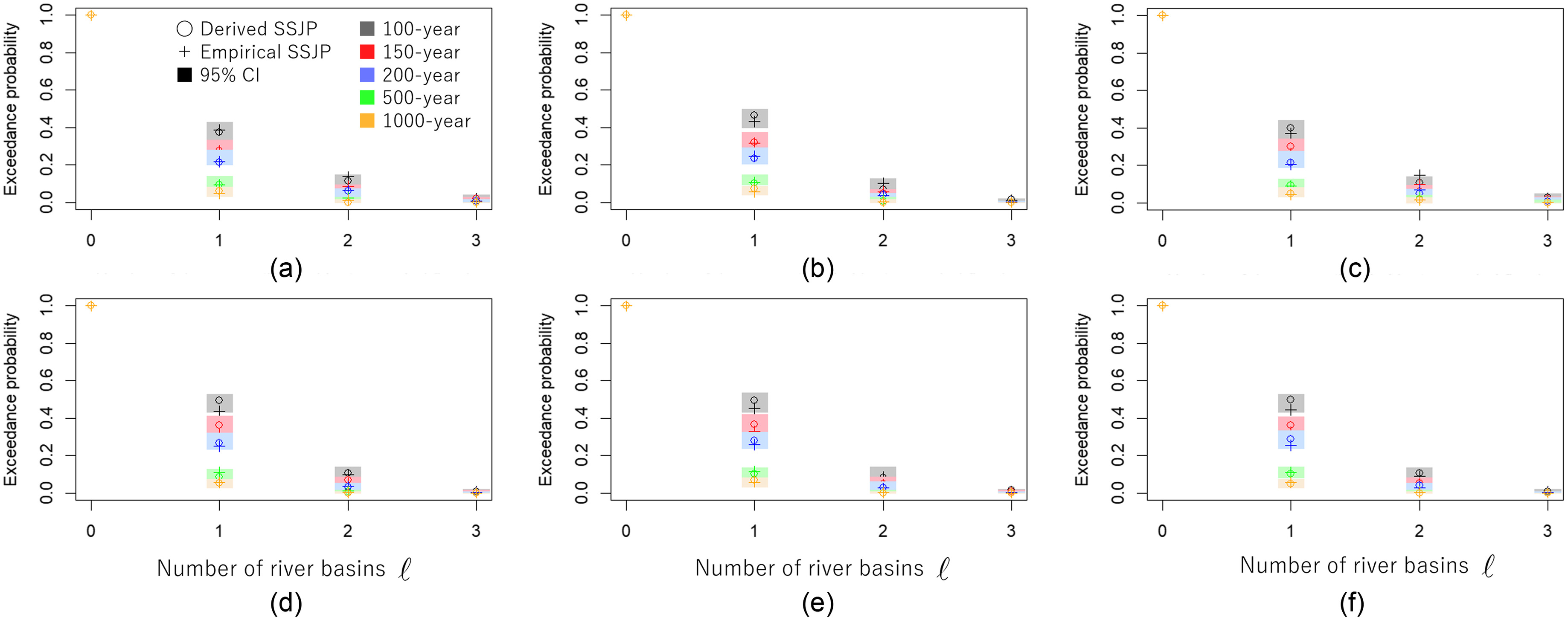
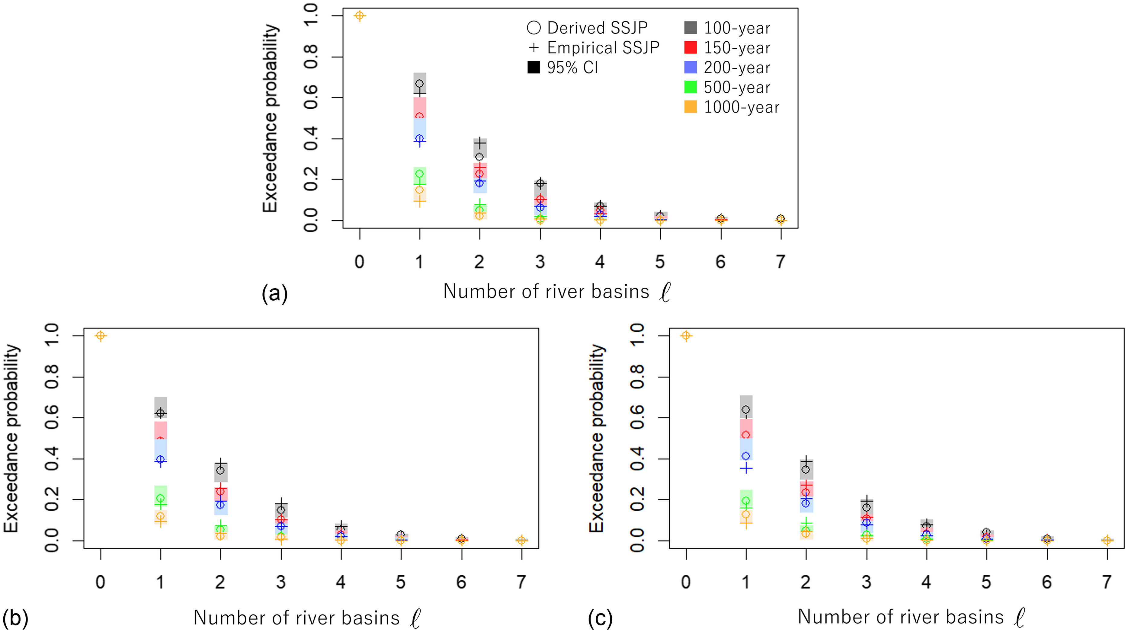
To derive the 95% CI of the derived SSJP, bootstrap sampling was performed; however, for 50% of the resampled data (500 out of 1,000 trials) in three-river cases, the fitted multivariate HR model did not satisfy the condition of partial correlation for three-river cases (and around 99% in seven-river cases); as a result, such trials were discarded. These selective samples forced making biased estimates of CIs with a far narrower range (see Fig. 9 for the distribution of bootstrap samples); therefore, the 95% CIs in Figs. 7 and 8 were derived by repeating the processes of empirical SSJP (Step 6) 1,000 times.
Discussions
In the preceding validation, an empirical CDF was created by counting the number of river basins where annual maximum river discharge exceeded the threshold return periods (100, 200, 500, and 1,000) in d4PDF data. Although the developed SSJP framework based on multivariate HR model was not fit to this higher-dimensional () empirical CDF and estimated by combining only pairwise dependencies in the bivariate HR models, the result showed acceptable agreement. This suggests that the proposed framework fairly works for estimating flood risk over catchment.
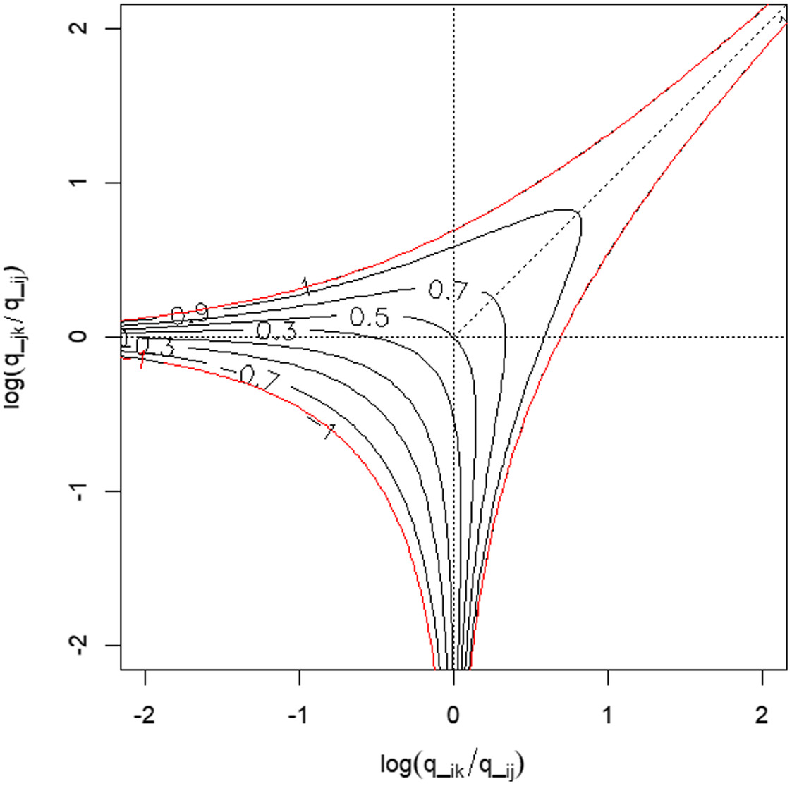
Whether or not the multivariate HR model is constructable from bivariate HR models depends on the combination of bivariate dependence parameters. Given the constraint of partial correlation , the dependence parameters needed to satisfy the following conditions:
(17)
The preceding parameter space is shown as a contour of on the 2D coordinate between and . According to Fig. 10, the conditions for Eq. (17) indicated that if one parameter was relatively small or large, the others must be similar. The similar value of the three inferred previously was located at around the origin in the figure. The higher the dimension, the harder it was to satisfy Eq. (17) for all the combinations of the three dependence parameters. Thus, the applicable number of rivers for the HR model declined, though the number actually increased from three to five dimensions simply due to the increasing number of total combinations. Eq. (17) is a simple but useful index to determine whether data satisfied the minimum requirements of the HR model.
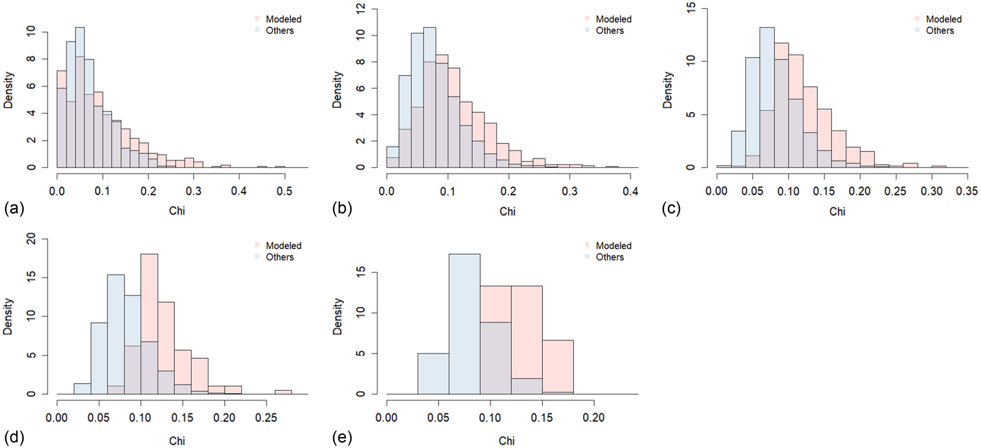
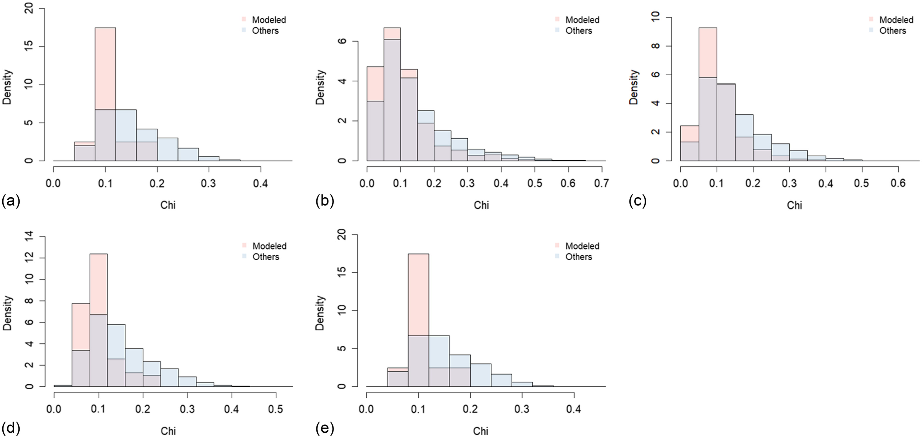
The histograms of mean and coefficient of variation (COV) of for the modeled combinations and others (some partial correlations were negative) in the range of three to seven dimensions are shown in Figs. 11 and 12, respectively. Overall, the mean values of were small. The modeled combinations showed relatively higher correlation coefficients. The COV values of were smaller for the modeled combinations. This tendency was clearer in larger dimensions. As discussed previously, a combination of similar partial correlations (around the origin of Fig. 10) falls within the parameter space for the HR model (the outer line in Fig. 10). On the other hand, among the applicable combinations in Figs. 7 and 8, all the river basins were not necessarily from the same major group in Fig. 5, but a few were from the other (e.g., one example per river basin was River 91, 93, 97, 98, 99, 101, and 105). In such a case, a partial correlation in some combinations fell into the limits of the allowable ranges in Fig. 10. In case of nested logistic (Coles and Tawn 1991) or nested negative logistic models (Kitano 2022), they can only express the dependence conditions where many pairs among all bivariate combinations share the same dependence structure, which is somehow a relaxed model rather than a logistic and negative logistic model with a single parameter. The HR model is considered as a more flexible model, whose total number of parameters is the number of pairs, and the relation of parameters values are less restrictive while still simple enough to analytically derive SSJP. In other words, the HR model can be an extension model by relaxing the nested model.
According to Fig. 5, the target catchments in Kyushu Island was classified into two groups of mutually correlated river basins: one faces the East China Sea (west side, Rivers 90–101) and the other is located on the Philippines Sea side (east side, Rivers 102–107). Heavy rainfall on the east side of the island is typically supplied by typhoons that generated on a path through the Philippines Sea, while that on the west side is more characterized by a seasonal frontal rain band (called Baiu) from June to July (MLIT 2015). The proportion of occurrence season of extreme river discharge () in d4PDF between the Baiu season (June or July) and the typhoon season (August or September) was investigated in Table 3. Among 20 river basins, Rivers 90–101 had more events in the Baiu season, while the typhoon season is more dominant for Rivers 102–107. Rivers 108 and 109 show a relatively higher ratio of occurrence in the Baiu season; therefore, the correlation was lower with Rivers 102–105 in the same group. The Ministry of Land, Infrastructure, Transport and Tourism (MLIT) reported that River 108 experiences heavy rainfall in both seasons (MLIT 2007b), while flood events in River 109 have been historically caused by typhoons (MLIT 2007a). Although inconsistency of flood occurrence season in River 109 may be caused by systematic bias of typhoons in d4PDF, overall characteristics of extreme flood seasons in Kyushu Island are expressed in d4PDF, which are clearly shown as mutually correlated groups of river basins in Fig. 5. This classification agreed with the rainfall-based hydrological regionalization by MLIT (2015). Hydrological classification has been also utilized in other case studies to efficiently construct high-dimensional dependence models in a literature (e.g., Quinn et al. 2019). As shown in Fig. 10, it is hard for the combination of high- and low-dependence parameters to satisfy the constraint of partial correlation coefficients. Therefore, it is suggested that a priori hydrological classification of target rivers may improve the feasibility of deriving SSJP using the multivariate HR model.
| River | Baiu season (%) | Typhoon season (%) |
|---|---|---|
| 90 | 0.6 | 0.4 |
| 91 | 0.51 | 0.49 |
| 92 | 0.65 | 0.35 |
| 93 | 0.64 | 0.36 |
| 94 | 0.6 | 0.4 |
| 95 | 0.56 | 0.44 |
| 96 | 0.62 | 0.38 |
| 97 | 0.62 | 0.38 |
| 98 | 0.75 | 0.25 |
| 99 | 0.84 | 0.16 |
| 100 | 0.77 | 0.23 |
| 101 | 0.8 | 0.2 |
| 102 | 0.26 | 0.74 |
| 103 | 0.28 | 0.72 |
| 104 | 0.26 | 0.74 |
| 105 | 0.33 | 0.67 |
| 106 | 0.35 | 0.65 |
| 107 | 0.46 | 0.54 |
| 108 | 0.68 | 0.32 |
| 109 | 0.60 | 0.40 |
Simulated river discharge data from d4PDF are known not to converge to the extreme value theory with the block size shorter than 20 years (Kitano 2022). Therefore, the uncertainty of the derived SSJP may be wider when applied to past observation data. Another limitation is that as the number of target river basins increases, the multivariate HR model gets harder to construct. As a result, a nonnegligible number of trials were discarded, when CIs could not be created from the rest of the samples because it leads to biased estimation. It is clarified that the strong regulation of partial correlation makes it hard to derive CIs when the HR model is applied to derive SSJP. Still, CIs estimated from empirical SSJP added on Figs. 7 and 8 provide supportive information of sampling uncertainty.
Conclusions
Intensified by global climate change, the compound risk of the co-occurrence of hydrological extremes, such as multiple-river flooding or simultaneous river and coastal flooding, receives high public attention. This study devised a multivariate HR model to estimate compound exceedance probabilities as the SSJP for a large number of river basins and tested its applicability based on extreme river discharge data from a large ensemble () of climate simulation data (d4PDF). The obtained findings are summarized as follows:
•
The SSJP was analytically derived from the multivariate HR model whose cumulative probability is also analytically computable.
•
Twenty-year block maxima data successfully converged to the multivariate HR model for several cases of two- to seven-river basins. In turn, stable application of multivariate extreme value distributions requires a large sample size that ensures a sufficient sample size for 20-year block maxima.
•
The SSJP and CIs get harder to obtain for the size of river basin with more than four rivers due to the limitation of partial correlation.
The successfully constructed multivariate HR model was composed of the river basin pairs with similar dependence structure. Nevertheless, the HR model was found to allow a different dependence structure to some extent and thus was more flexible than the nested logistic or negative logistic model, which requires the same dependence structure among variables.
Overall, this study demonstrated promising results for applying the HR model to the co-occurrence of multiple river flooding under certain conditions. The large ensemble of d4PDF substantially ensured the convergence of the data to asymptotic theory, which contributed to robust compound risk assessments. In a bivariate case, Kitano (2022) has already revealed that observation record length is not enough to robustly identify tail dependency. Owing to the sample size secured by d4PDF, the preceding applicability (and limitation) of the SSJP based on the HR model was derived. The systematic bias in d4PDF was removed by Kobayashi et al. (2020); however, estimated tail dependency is based on climate simulations. Future study will cross-check the joint flood risk based on both observed and simulated data and explore climate change impact by applying the methodology to future climate projections.
Data Availability Statement
Some or all data, models, or code that support the findings of this study are available from the corresponding author upon reasonable request.
Acknowledgments
This work was supported by the MEXT Program for the Advanced Studies of Climate Change Projection (SENTAN) Grant No. JPMXD0722678534 funded by the Ministry of Education, Culture, Sports, Science, and Technology, Japan (MEXT). This study used d4PDF produced jointly with the Earth Simulator by science programs (SOUSEI, TOUGOU, SI-CAT, DIAS) of MEXT, Japan. This data set was collected and provided by the Data Integration and Analysis System (DIAS) (Project No. JPMXD0716808999), developed and operated by MEXT.
References
Boldi, M. O., and A. C. Davison. 2007. “A mixture model for multivariate extremes.” J. R. Stat. Soc. B 69 (2): 217–229. https://doi.org/10.1111/j.1467-9868.2007.00585.x.
Centre for Ecology and Hydrology. 1999. Flood estimation handbook. Wallingford, UK: Centre for Ecology and Hydrology.
Coles, S. G., and J. A. Tawn. 1991. “Modeling extreme multivariate events.” J. R. Stat. Soc. B 53 (2): 377–392. https://doi.org/10.1111/j.2517-6161.1991.tb01830.x.
Cooley, D., R. A. Davis, and P. Naveau. 2010. “The pairwise beta distribution: A flexible parametric multivariate model for extremes.” J. Multivar. Anal. 101 (9): 2103–2117. https://doi.org/10.1016/j.jmva.2010.04.007.
Dey, D. K., and J. Yan. 2016. Extreme value modeling and risk analysis—Methods and applications. Boca Raton, FL: CRC Press.
Diederen, D., Y. Liu, B. Gouldby, F. Diermanse, and S. Vorogushyn. 2019. “Stochastic generation of spatially coherent river discharge peaks for continental event-based flood risk assessment.” Nat. Hazards Earth Syst. Sci. 19 (5): 1041–1053. https://doi.org/10.5194/nhess-19-1041-2019.
Engelke, S., and A. S. Hitz. 2020. “Graphical models for extremes.” J. R. Stat. Soc. B 82 (4): 871–932. https://doi.org/10.1111/rssb.12355.
Engelke, S., A. Malinowski, Z. Kabluchko, and M. Schlather. 2015. “Estimation of Husler-Reiss distributions and Brown-Resnick processes.” J. R. Stat. Soc. B 77 (1): 239–265. https://doi.org/10.1111/rssb.12074.
Feller, W. 1957. An introduction to probability theory and its applications. New York: Wiley.
Heffernan, J. E., and J. A. Tawn. 2004. “A conditional approach for multivariate extreme values.” J. R. Stat. Soc. B 66 (3): 497–546. https://doi.org/10.1111/j.1467-9868.2004.02050.x.
Husler, J., and R. D. Reiss. 1989. “Maxima of normal random vectors—Between independence and complete dependence.” Stat. Probab. Lett. 7 (4): 283–286. https://doi.org/10.1016/0167-7152(89)90106-5.
Ishii, M., and N. Mori. 2020. “d4PDF: Large-ensemble and high-resolution climate simulations for global warming risk assessment.” Prog. Earth Planet. Sci. 7 (1): 1–22. https://doi.org/10.1186/s40645-020-00367-7.
Keef, C., J. Tawn, and C. Svensson. 2009. “Spatial risk assessment for extreme river flows.” J. R. Stat. Soc. C 58 (5): 601–618. https://doi.org/10.1111/j.1467-9876.2009.00672.x.
Kitano, T., 2022. “Spatial dependence analysis of extreme wave heights by employing nested model for cross occurrence rate.” [In Japanese.] J. Jpn. Soc. Civ. Eng. Ser. B2 78 (2): I_91–I_96. https://doi.org/10.2208/kaigan.78.2_I_91.
Kobayashi, K., T. Tanaka, M. Shinohara, and Y. Tachikawa. 2020. “Analyzing future changes of extreme river discharge in Japan using d4PDF.” [In Japanese.] J. Jpn. Soc. Civ. Eng. Ser. B1 76 (1): 140–152. https://doi.org/10.2208/jscejhe.76.1_140.
Kotz, S., and S. Nadarajah. 2000. Extreme value distributions: Theory and applications. London: Imperial College Press.
Mizuta, R., et al. 2017. “Over 5,000 years of ensemble future climate simulations by 60-km global and 20-km regional atmospheric models.” Bull. Am. Meteorol. Soc. 98 (7): 1383–1398. https://doi.org/10.1175/BAMS-D-16-0099.1.
MLIT (Ministry of Land, Infrastructure, Transport, and Tourism). 2007a. “Masterplan of the Kimotsuki River System.” Accessed October 27, 2023. http://www.qsr.mlit.go.jp/osumi/river/chisui/pdf/kihonhoushin.pdf.
MLIT (Ministry of Land, Infrastructure, Transport, and Tourism). 2007b. “Masterplan of the Sendai River System.” Accessed October 27, 2023. https://www.mlit.go.jp/river/shinngikai_blog/shaseishin/kasenbunkakai/shouiinkai/kihonhoushin/070223/pdf/s5-3.pdf.
MLIT (Ministry of Land, Infrastructure, Transport, and Tourism). 2015. “Guideline of probable maximum precipitation for fluvial and pluvial flood hazard mapping.” Accessed October 27, 2023. https://www.mlit.go.jp/river/shishin_guideline/pdf/shinsuisoutei_honnbun_1507.pdf.
MLIT (Ministry of Land, Infrastructure, Transport, and Tourism). 2018. “Economic damage by heavy rainfall in July, 2018.” Accessed October 27, 2023. https://www.mlit.go.jp/common/001252521.pdf.
MLIT (Ministry of Land, Infrastructure, Transport, and Tourism). 2019. “Economic damage by Typhoon Hagibis, 2019 (50th report).” Accessed October 27, 2023. https://www.mlit.go.jp/common/001319108.pdf.
MLIT (Ministry of Land, Infrastructure, Transport, and Tourism). 2023. “Masterplan and river improvement plan.” Accessed October 27, 2023. https://www.mlit.go.jp/river/basic_info/jigyo_keikaku/gaiyou/seibi/index.html.
Mostofi Zadeh, S., M. Durocher, D. H. Burn, and F. Ashkar. 2019. “Pooled flood frequency analysis: A comparison based on peaks-over-threshold and annual maximum series.” Hydrol. Sci. J. 64 (2): 121–136. https://doi.org/10.1080/02626667.2019.1577556.
Neal, J., C. Keef, P. Bates, K. Beven, and D. Leedal. 2013. “Probabilistic flood risk mapping including spatial dependence.” Hydrol. Process 27 (9): 1349–1363. https://doi.org/10.1002/hyp.9572.
Quinn, N., P. D. Bates, J. Neal, A. Smith, O. Wing, C. Sampson, J. Smith, and J. Heffernan. 2019. “The spatial dependence of flood hazard and risk in the United States.” Water Resour. Res. 55 (3): 1890–1911. https://doi.org/10.1029/2018WR024205.
Sasaki, H., K. Kurihara, I. Takayabu, and T. Uchiyama. 2008. “Preliminary experiments of reproducing the present climate using the non-hydrostatic regional climate model.” Sola 4: 25–28. https://doi.org/10.2151/sola.2008-007.
Sharma, S., and P. P. Mujumdar. 2022. “Modeling concurrent hydroclimatic extremes with parametric multivariate extreme value models.” Water Resour. Res. 58 (2): e2021WR031519. https://doi.org/10.1029/2021WR031519.
Solari, S., and M. A. Losada. 2012. “A unified statistical model for hydrological variables including the selection of threshold for the peak over threshold method.” Water Resour. Res. 48 (10): WR011475. https://doi.org/10.1029/2011WR011475.
Stephenson, A. G. 2002. “Extreme value distributions.” R News 2 (2): 31–32.
Tanaka, S., K. Takara, A. Snorrason, H. Finnsdottir, and E. M. Moss. 2002. A study on threshold selection in POT analysis of extreme floods, 299–306. Wallingford, UK: IAHS Publication.
Tanaka, T., and T. Kitano. 2021. “An application of multivariate extreme value distribution to d4PDF: Co-occurrence probability of extreme floods in two river basins.” Appl. Stat. 50 (2–3): 75–101. https://doi.org/10.5023/jappstat.50.75.
Tanaka, T., and T. Kitano. 2022. “An application of multivariate extreme value distribution to d4PDF: co-occurrence probability of extreme floods in two river basins.” Ouyou Toukeigaku 50 (2–3): 2021.
Tanaka, T., K. Kiyohara, and Y. Tachikawa. 2020. “Comparison of fluvial and pluvial flood risk curves in urban cities derived from a large ensemble climate simulation dataset: A case study in Nagoya, Japan.” J. Hydrol. 584 (May): 124706. https://doi.org/10.1016/j.jhydrol.2020.124706.
Tanaka, T., K. Kobayashi, and Y. Tachikawa. 2021. “Simultaneous flood risk analysis and its future change among all the 109 class-A river basins in Japan using a large ensemble climate simulation database d4PDF.” Environ. Res. Lett. 16 (7): 074059. https://doi.org/10.1088/1748-9326/abfb2b.
Tanaka, T., and Y. Tachikawa. 2015. “Testing the applicability of a kinematic wave-based distributed hydrological model in two climatically contrasting catchments.” Hydrol. Sci. J. 60 (7–8): 1361–1373. https://doi.org/10.1080/02626667.2014.967693.
Wahl, T., S. Jain, J. Bender, S. D. Meyers, and M. E. Luther. 2015. “Increasing risk of compound flooding from storm surge and rainfall for major US cities.” Nat. Clim. Change 5 (12): 1093–1097. https://doi.org/10.1038/nclimate2736.
Zellou, B., and H. Rahali. 2019. “Assessment of the joint impact of extreme rainfall and storm surge on the risk of flooding in a coastal area.” J. Hydrol. 569 (Feb): 647–665. https://doi.org/10.1016/j.jhydrol.2018.12.028.
Zscheischler, J., et al. 2018. “Future climate risk from compound events.” Nat. Clim. Change 8 (6): 469–477. https://doi.org/10.1038/s41558-018-0156-3.
Information & Authors
Information
Published In

Journal of Hydrologic Engineering
Volume 29 • Issue 3 • June 2024
Copyright
This work is made available under the terms of the Creative Commons Attribution 4.0 International license, https://creativecommons.org/licenses/by/4.0/.
History
Received: Apr 18, 2023
Accepted: Dec 18, 2023
Published online: Feb 29, 2024
Published in print: Jun 1, 2024
Discussion open until: Jul 29, 2024
Authors
Metrics & Citations
Metrics
Citations
Download citation
If you have the appropriate software installed, you can download article citation data to the citation manager of your choice. Simply select your manager software from the list below and click Download.