The workflow proposed to assess the feasibility of using streamflow simulated from a hydrologic model to estimate flow-frequency statistics is outlined as follows:
Step 1: Model output location and stream gauge matching.
Step 2: Candidate stream gauge screening.
Step 3: Streamflow record matching.
Step 4: Computation of streamflow frequency statistics.
Step 5: Scaling correction.
Step 6: Initial bias computation.
Step 7: GAM fitting.
Step 8: Bias correction.
Step 9: Workflow evaluation.
Step 10: Uncertainty analysis.
The generalized workflow is described subsequently, and the section “Practical Application of the Workflow” demonstrates the practical application of this workflow to the computation of LFF statistics from simulated streamflow provided by Robinson et al. (
2020). A suite of scripts (
Whaling et al. 2022) were written in the R language (
R Core Team 2022) as companion software to this paper and provide publicly accessible and reproducible procedures and computations for all data preparation, manipulation, and results following Steps 1–10 specific to the practical application.
Step 5: Scaling Correction
A key aspect of the proposed workflow is to help ensure comparability between simulated and gauged flow frequency statistics for a reliable bias assessment and correction. All model output locations are unlikely to coincide where there is gauged streamflow available for direct comparison. Despite enforcing a maximum allowable log-ratio (absolute value) of the CDA in Step 2, any stream gauge-model pair having a log-ratio greater than zero is still not directly comparable because that implies the CDAs do not agree exactly and therefore neither do the watersheds. The drainage-area ratio (DAR) method (
Hirsch 1979;
Asquith et al. 2006) is typically used to estimate streamflow at an ungauged location by using streamflow from a nearby stream gauge with the assumption that the relation between streamflows at the ungauged and gauged sites are equivalent to the ratio of the drainage areas; in the context of this workflow, it is used to scale the gauged statistic to the model output location with a correspondingly smaller or larger CDA. The DAR method is expressed as:
where
= scaled gauged NQT statistic [cubic length (L) per time (
)] for the ungauged (model output) location;
= NQT statistic (
) for the stream gauge;
= cumulative drainage area (
) for the ungauged (model output) location;
= cumulative drainage area (
) for the stream gauge; and
= exponent of unity. The value for
is often assumed equal to 1, although Asquith et al. (
2006) investigated this assumption and found that
ranged from 0.700 to 0.935 for daily mean streamflows in Texas, and work by Asquith and Thompson (
2008) found that
moved away from unity for peak streamflows in Texas.
Reformulating Eq. (
1) for estimation of flow-frequency statistics in base-10 logarithm units (all log-transformations in this paper are base-10 logarithms), the gauged LFF statistics are scaled to the same measure space of the simulated streamflow using Eq. (
2):
where
= gauged LFF statistic [
] computed without any adjustments;
= CDA (
) at the simulated streamflow model output location;
= CDA (
) at the stream gauge location; and
= flow-frequency statistic [
] for the stream gauge scaled by the CDA ratio.
Step 6: Initial Bias Computation
During Step 6, biases present initially in the simulated streamflow statistics (without a bias correction) are investigated to inform the practitioner how the simulated flow-frequency statistics compare with their gauged counterparts. The initial biases in the NQT statistic,
[units of
] [Eq. (
3)], are computed by subtracting the simulated flow-frequency statistics from the corresponding gauged flow-frequency statistics (adjusted with the DAR method in Step 5) in base-10 logarithm-space for each
of
stream gauge-model pairs in the comparison data set given by
The practitioner could use the initial biases to determine the average magnitude and direction of the bias in the simulated flow-frequency statistics. The mean initial bias, formulated by Eq. (
4), is simply the arithmetic mean of
[Eq. (
3)] shown by the number of
stream gauge-model pairs
Another diagnostic useful for interpreting the initial biases,
[units of squared
] is computed by taking the average of squared deviations for each
observation of
stream gauge-model pairs from a zero-mean bias
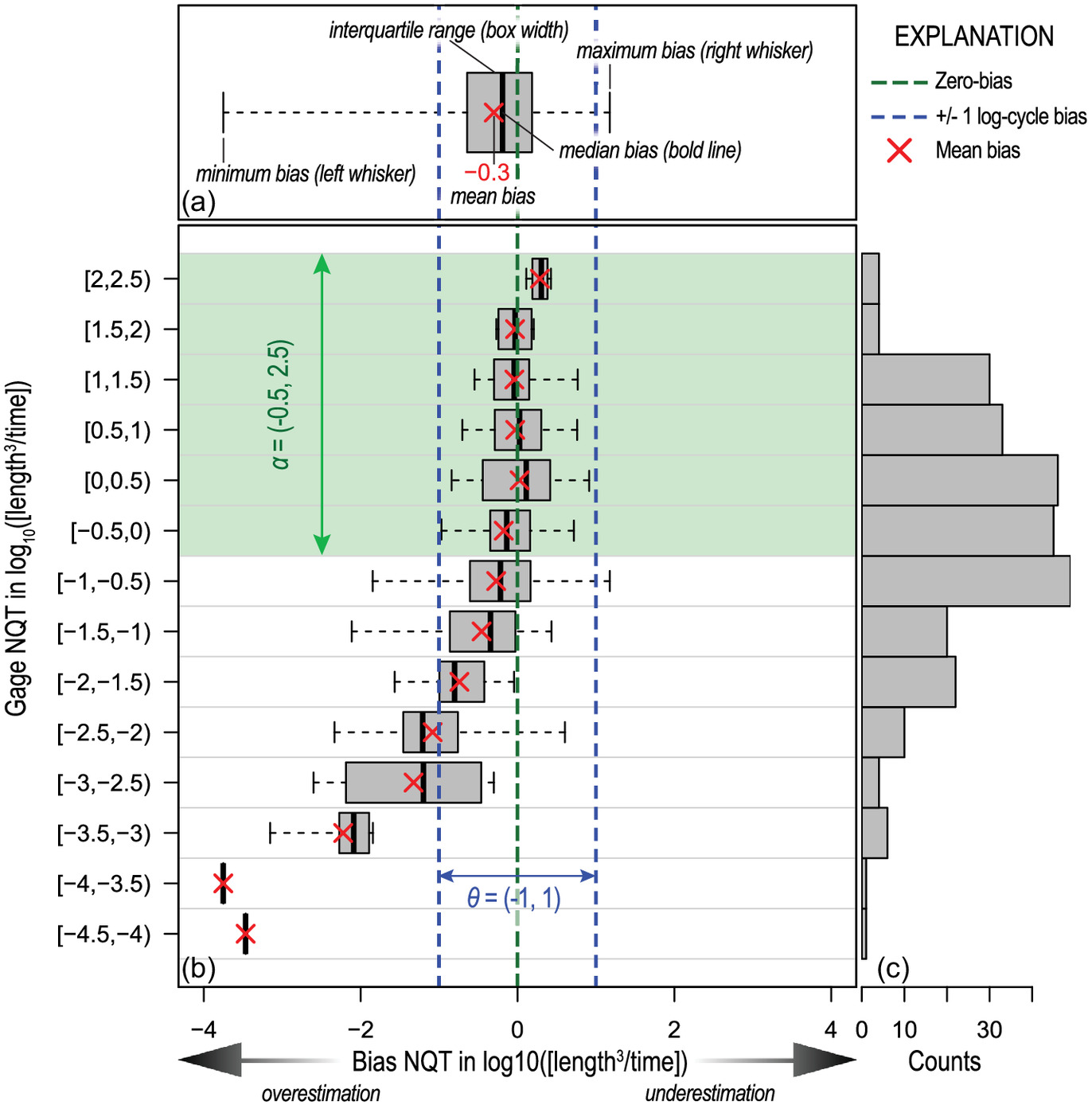
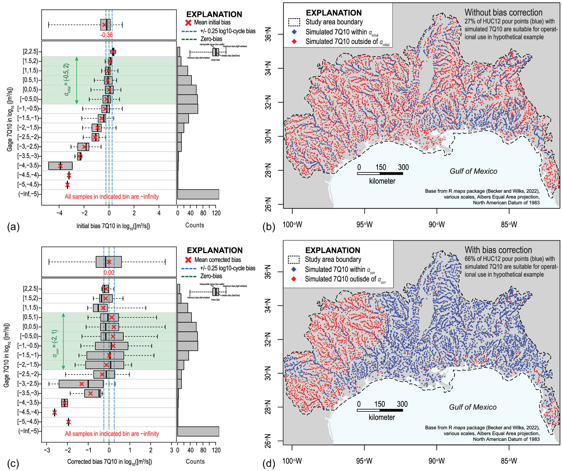
It is also important to investigate the existence of a dependent relation between the magnitude of the gauged flow-frequency statistic and the magnitude of the initial bias. As discussed in the “Introduction,” this workflow is premised on the expectation that hydrologic models generally do not reliably predict into the tails of the streamflow distribution. Thus, when simulated streamflows are cast into a flow magnitude for a selected frequency, the bias magnitude is likely to be larger for the extremely large and small magnitudes. Graphically, the relation is investigated with box and whisker plots (
Chambers et al. 1983) of the bias binned by the magnitude of the gauged flow-frequency statistic (scaled by CDA ratio,
) (Fig.
3) and quantitatively assessed by recomputing
for each bin (plotted as red X symbols).
Compared with the bias direction and magnitude shown by all stream gauge-model pairs [Fig.
3(a)], the individual box plots give a sense of the variability in the bias direction and magnitude with respect to binned magnitudes of the gauged flow-frequency statistic [Fig.
3(b)] and the number of observations in each bin [Fig.
3(c)]. All binned
values are ideally centered near zero, indicating the simulated flow-frequency statistics are unbiased for all magnitudes of flow-frequency represented in the comparison data set. Binned
values that plot to the left (negative values) and right (positive values) of the zero-bias line indicate the simulated flow-frequency statistics are being overestimated and underestimated, respectively. The bin interval (0.5 in the example shown in Fig.
3) is user-defined and depends on the range and sample size of the gauged flow-frequency statistic present in the stream gauge-model pairs; Sturges’ rule for determining the number of bins (
Scott 2009) is used throughout this paper.
In terms of assessing the reliability of the simulated streamflow statistics, the binned box plots are useful for defining a number, , that specifies an interval range of the magnitude of gauged flow-frequency statistics—and by extension simulated flow-frequency statistics—considered to be unbiased. More generally, defines the magnitude range of the (initial or bias-corrected) simulated flow-frequency statistics the practitioner deems reliable for operational use; we use to denote the range determined for the initial biases and to denote the range determined for the corrected biases (more details provided in Step 9).
A modified box and whisker plot shown in Fig.
3 demonstrates how
is visually determined from the plotted initial (or corrected) biases. A specification of
equal to
indicates that the simulated NQT statistics are reliable for any magnitude greater than
and less than 2.5 base-10 logarithms of streamflow. The left and right bounds for
come from the relation of the binned biases on the
-axis with
, a user-defined cut-off value for designating how much bias is too much. Expressed as an interval range,
is the cut-off value around a bias of zero base-10 logarithms of streamflow. Accordingly, biases shall not exceed
log-cycle (order of magnitude) of difference when
is arbitrarily equal to one in the example. Therefore, the left bound for
(
) is from the lower interval of the smallest
-axis bin where the absolute value of minimum and maximum binned biases on the
-axis do not exceed one. Similarly, the right bound for
(2.5) is from the upper interval of the largest
-axis bin where the absolute value of minimum and maximum binned biases on the
-axis do not exceed one. However, the practitioner could use descriptive statistics other than the binned minima and maxima indicated by the box and whisker plots, such as the median, mean, or interquartile range, relative to
.
One last comment is needed. Even if for the uppermost bin is unbiased, a right bound of (infinity) is not recommended because it incorrectly implies that simulated flow-frequency statistics of any magnitude are valid despite not being captured in the stream gauge-model pairs. The same logic dictates that a lower bound of would be invalid. In such cases, the largest gauged NQT statistic is suggested for the right bound, and the smallest for the left bound. However, biases are to be expected, and the remaining steps demonstrate the computation and application of a bias correction to the simulated flow frequency statistics to see if biases initially present can be mitigated.
Step 7: GAM Fitting
The characteristics of the bias shown by each NQT flow-frequency statistic are investigated by fitting thin-plate cross-validated splines to all
values using GAMs (
Wood 2003,
2011) in R (
R Core Team 2022) using the
mgcv package (
Wood 2021). The GAMs are fit in two stages: Stage I is aimed at removing spatial biases that result from unmeasured covariates or structural flaws in the model that produced the simulated streamflow, and Stage II is designed to add information about the stream network back into a total bias correction. The spatial component of the Stage I GAM fitting removes information about the network, so a residual bias is assumed present that is a function of the magnitude of the simulated flow-frequency statistic, hence the need for the Stage II GAM.
The proposed two-stage GAM fitting assumes that the simulated-streamflow modeling technique preserved information about the network. Thus, the two-stage GAM fitting produces two sets of bias-correction values needed for a total bias-correction in Step 8: Stage I produces the spatial bias corrections, , and Stage II produces the residual bias corrections, . Computation of each is discussed in more detail next.
Stage I GAM Fitting
Stage I GAM fitting generates predictions of the spatial-bias correction,
. Eq. (
6) is a simple GAM framework that provides a rapid and effective framework to fit a surface to the stream gauge-model pair biases for each NQT flow-frequency statistic
At a minimum, all that is needed to explain the biases is the smooth [
function] (
Wood 2003,
2011) on the stream gauge-model pair’s two-dimensional coordinate measured as the Universal Transverse Mercator (UTM) northing and easting; with this simple framework, the Stage I GAMs therefore represent the smoothing of the simulated streamflow model residuals in the domain of each flow-frequency statistic.
The spatial GAMs do not require any prior knowledge of the functional form of the bias and can mimic potential curvatures in data with the overall functional form while still retaining additive components. An attractive feature is that they grant flexibility to the user to account for watershed properties and or other factors not originally used as covariates in the hydrologic model. Testing of compound GAM frameworks with different distribution families (Gaussian assumed by default) and or terms in addition to the simple spatial smooth is a necessary step to this workflow if there is a strong reason to do so. Guidance for choosing an appropriate GAM framework is provided by Wood (
2020).
For comparisons between frameworks for model selection, the reported deviance explained and Akaike information criterion (AIC) (
Akaike 1974) are used as a measurement of goodness of fit after Asquith et al. (
2017) and Dey et al. (
2016), and references therein.
Predictions of
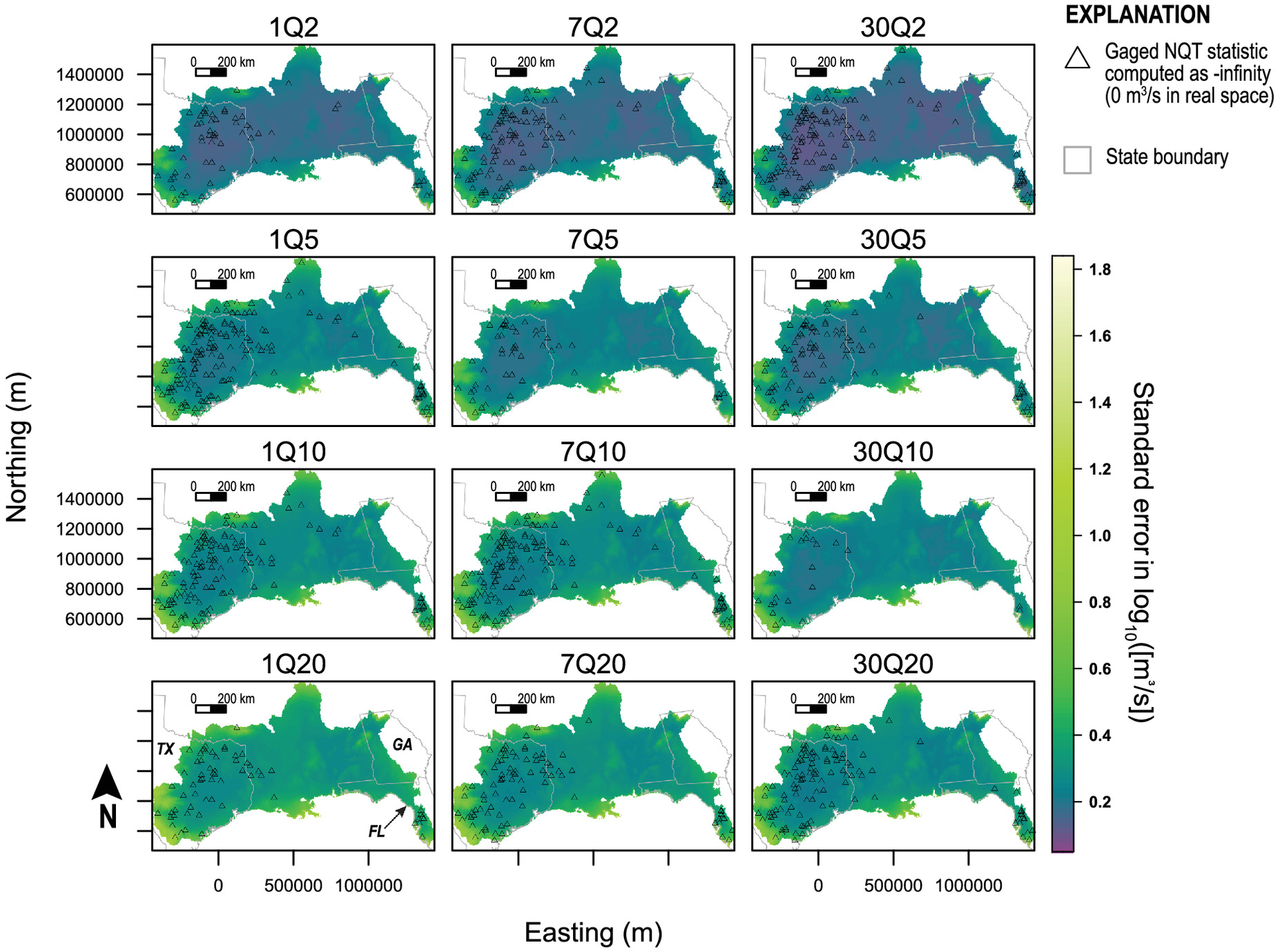
are determined from the Stage I GAM given a set of values for the framework terms. For the simple framework, all that is needed are the eastings and northings of grid cell locations from a gridded data set (raster) where predictions are needed. The raster extent needs to encompass the spatial coverage of the stream gauge-model locations. The gridded predictions result in a surface spanning the study area that are interrogated for the spatial bias-correction values for gauged (and ungauged) model output locations. Similarly, GAM standard errors of fit, which are based on the posterior distribution of the smoothing function coefficients (
Wood 2021), are predicted onto the same grid for an assessment of the uncertainty with respect to space in Steps 9 and 10.
Stage II GAM Fitting
The second stage of GAM fitting removes the residual bias,
, that is present after Stage I GAM fitting and subsequent application of the spatial bias correction. A residual bias is assumed because the spatial smooth term in Eq. (
6) removes information about the stream network. The residual bias in the NQT flow-frequency statistic is computed following Eq. (
7) for each
of
stream gauge-model pairs:
where the spatial bias correction
is the cell value from gridded predictions made by Stage I GAM corresponding to the NQT flow-frequency statistic of interest (for example, use the 7Q2 raster to correct the initial simulated 7Q2) at some easting and northing of each stream gauge-model pair location. The raster cell value at the model output location is determined with GIS software or geospatial functions as implemented by Whaling et al. (
2022).
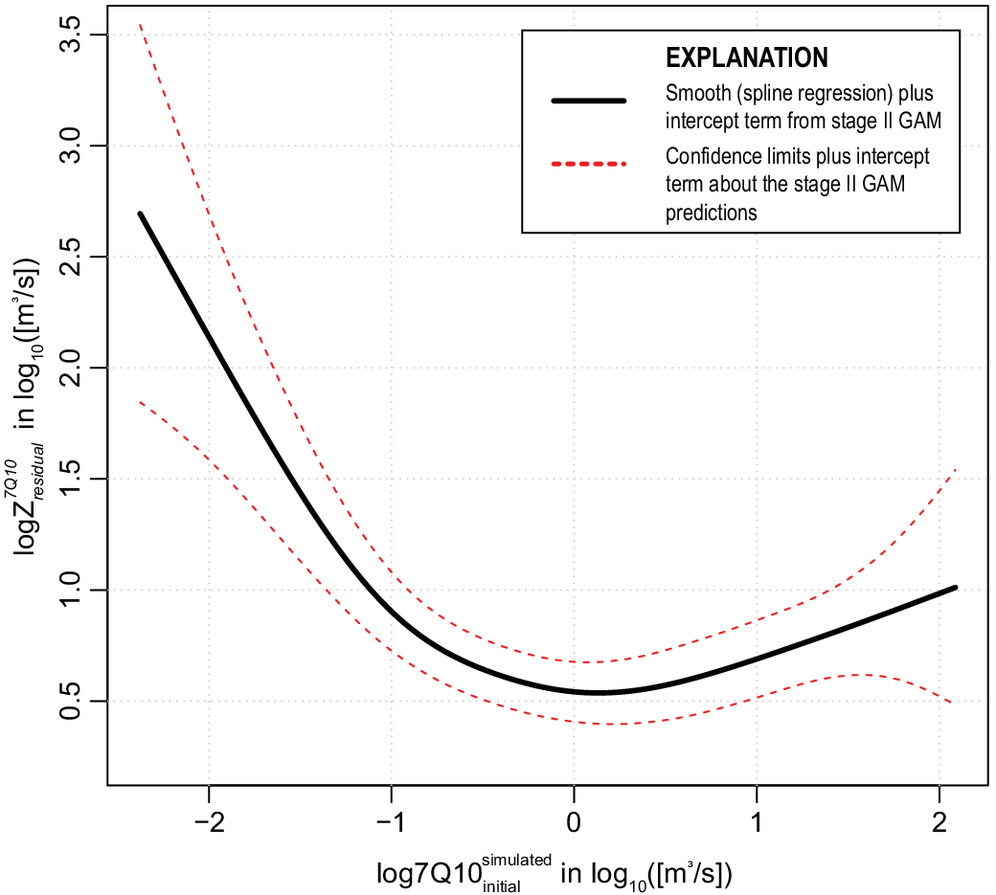
The second-stage GAM is then fitted from the resulting stream gauge-model residual bias with the following framework, which assumes a Gaussian distribution family on all finite values of
:
The fitted Stage II GAM produces a smooth (spline regression) that relates the magnitude of to a prediction for , with accounting for the intercept term output from the fitted GAM. Extrapolation to and with linear interpolation is suggested in the event that the stream gauge-model pairs do not encompass the extrema of .
Step 9: Workflow Evaluation
As a first-order evaluation, the corrected bias (
), mean corrected bias (
), and the bias-corrected variance from a mean bias of zero,
, is recomputed for the NQT statistic following Eqs. (
3)
–(
5), respectively, by replacing all values of
in the equations with the values of
[Eq. (
10)] determined for the stream gauge-model comparison data set. Values closer to zero are desired because it indicates the workflow effectively removed modeling residuals. However, where biases remain, the efficacy of the two-stage GAM process in removing the bias needs to be thoroughly evaluated, and further guidance is detailed subsequently.
Once a GAM framework has been selected that minimizes (absolute value), the practitioner can return to Step 8 and compute bias-corrected LFF statistics for all model output locations with simulated streamflow in the study area. Then, the workflow evaluation is focused on determining if the bias predictions apply to all bias-corrected flow-frequency statistics.
In terms of assessing the reliability of the bias-corrected simulated streamflow statistics, binned box plots, as suggested in Step 6, are useful. Similar to , is defined to specify the magnitude range of the bias-corrected simulated flow-frequency statistics considered as reliable for operational use, assuming that biases are still present after the correction scheme.
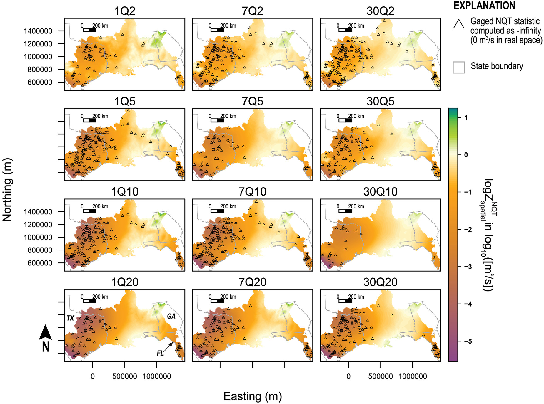
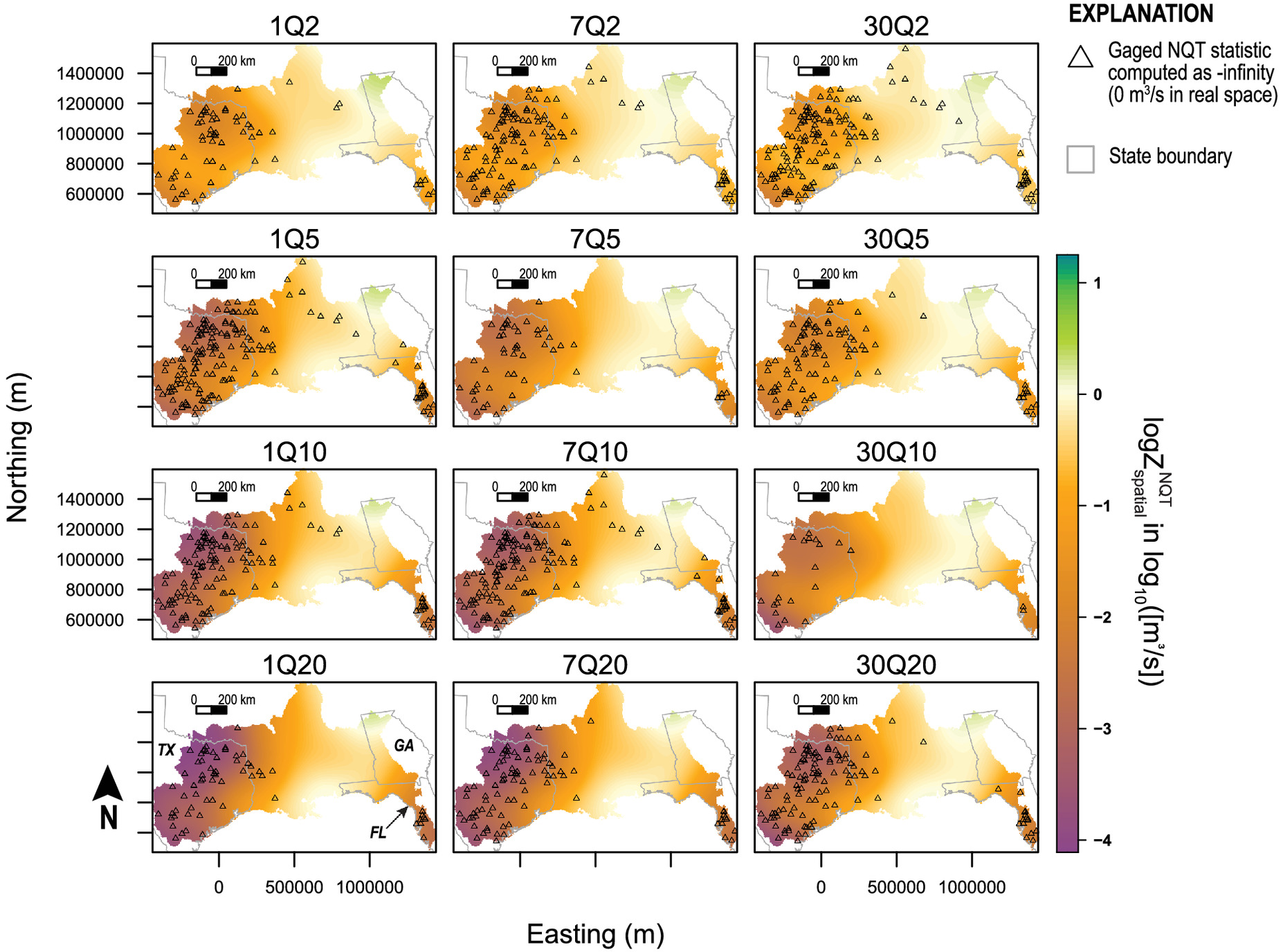
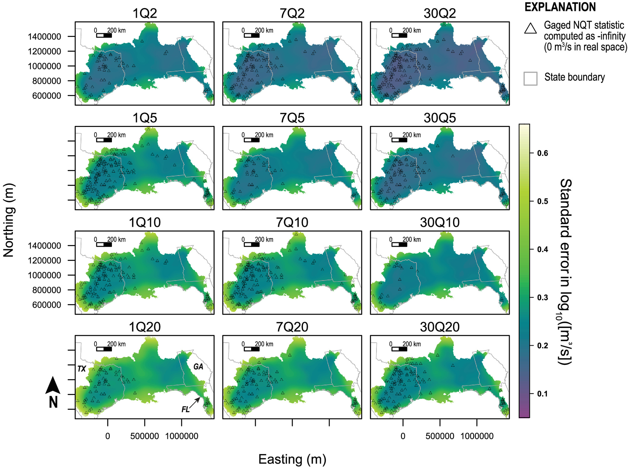
The first-stage GAM is used to explore the magnitude and spatial distribution of the spatial bias exhibited by the simulated flow-frequency statistics. Generally, maps of the spatial bias reveal where underestimation and overestimation occur in the study area and may provide conceptual feedback for testing of additional covariates in a compound Stage I GAM framework. Evaluation of the maps of the standard errors of fit (Step 7) are suitable for the semi-quantitative discussion about relative spatial GAM performance throughout the study area. In particular, they may help identify where estimates are unreliable because of poor stream gauge-model density.
Step 10: Uncertainty Analysis
Reporting of uncertainty is a necessary step in this workflow. The outcome of Step 10 is the production of some type of credible prediction limits unique for each modeling location in the domain of the desired statistic. To clarify, the computed 95% prediction limits for any one prediction do not provide a span containing the true mean statistic value with 95% probability but rather the limits so constructed to encompass the statistic 95% of the time (
Good and Hardin 2012).
The uncertainty analyses used for computation of 95% prediction limits is algorithmically straightforward although subject to several assumptions and ignored terms. A normal distribution of the log-transformed predictions is assumed applicable, and the final flow-frequency statistic is its mean. The applicable standard deviation is thus the core of the problem.
The variance of the predictions is assumed to stem from two sources, the statistical variance of the flow-frequency statistic and the two-stage GAM bias-prediction variance. Other sources of uncertainty are assumed negligible. Using a bootstrapping technique from Efron and Tibshirani (
1985), the statistical variance for each,
, simulated NQT LFF statistic,
, is estimated from a simulated population of the NQT statistic of interest. To create the simulated population, first, a sampled time series of flows is generated from the original time series intended for the flow-frequency analysis. Random sampling with replacement is recommended so that the sampled series size is equal to the size of the original series. Then, the NQT statistic is computed from the sample using the same methodology the user opted to employ in Step 4. The simulation is repeated many times (ideally thousands), and the desired statistical variance is computed from the simulated population.
The distribution and method of parameter estimation choices specific to the computation of the desired flow-frequency statistics are assumed to be correct in this workflow. However, Asquith et al. (
2017) discussed estimation difficulties with frequency analyses wherein additional uncertainties stem from the choice of the parameter probability distribution among reasonable candidates, and differing methods of parameter estimation (product moments, L-moments, maximum likelihood, and maximum product of spacing) will estimate differing distribution parameters for the same sample.
Uncertainty in the bias corrections can be conceptualized in several ways and, two options are provided. The bias corrections themselves are assumed as correct with only uncertainty stemming from prediction specific computations from the GAMs, and each prediction has a unique associated variance. Alternatively, bias corrections are assumed as incorrect and any residual bias in
contributes to a global variance in the final bias-corrected simulated flow-frequency statistic. The derivation may depend on the distribution family supplied in the spatial GAM framework. For the Gaussian case, the global scale of the GAM and its standard errors of fit (Step 7) unique for each prediction are combined through the salient mathematics of prediction intervals for a GAM (
Asquith 2020 and software documentation therein). Alternatively, the variance of
from a mean bias of zero,
, may serve as a reasonable estimate for a global GAM prediction variance. The formulation is structurally identical with that of
in Eq. (
5).
The two aforementioned variances, namely, statistical from the flow-frequency computations,
, and bias-correction from the Stage I and II GAM predictions,
, are used to compute
, the standard deviation for an individual simulated flow-frequency statistic,
, following Eq. (
11)
In the preceding equation, if is specified as , then the second term is a constant for all (NQT) simulated flow-frequency statistics.
Using the result of
, the 2.5% and 97.5% quantiles are computed from the normal distribution, which together represent the 95% prediction limits. One last caveat is needed. The uncertainty approach here does not attempt to propagate uncertainty into the flow-frequency statistic from the simulated daily values themselves. For example, the 95% prediction limits from Robinson et al. (
2020) would generally be too small because of variance reduction inherent to simulated streamflow from data-driven hydrologic models. Furthermore, the proposed computation of uncertainty is flexible so that it can be applied to comparisons between multiple simulated streamflow data sets that are being explored for operational use, especially given that model uncertainties are not reported in a standardized way, or they might not be reported at all.