Abstract
Water resources are crucial for human activities and sustainable socioeconomic development. Understanding surface water information can play a key role in water resource management, which affects the global water cycle and ecological environments. Considering the Hailar River water body as an example, this study proposes a new threshold self-learning water body extraction method (TSLWEM) based on modified normalized difference water index (MNDWI) data. The optimal water extraction thresholds determined by the TSLWEM algorithm for four test images were , 0, 0.1990, and . The TSLWEM algorithm effectively identified the target water body with recognition accuracies of 98.08%, 99.93%, 93.39%, and 93.20% for the four test images. Moreover, it can accurately identify small tributaries, such as lakes and rivers. The TSLWEM algorithm is suitable for Landsat 8 Operational Land Imager (OLI) data, which can effectively monitor and map complex surface water in temperate and semiarid regions while improving the accuracy of water body identification. The study’s findings provide technical support for the protection of water resources as well as their rational utilization and monitoring.
Introduction
Watersheds and lakes in the semiarid climatic region of northern China play an important role in connecting the natural water cycle and human economic activity. In semiarid areas, due to flat and wide riverbeds and a high degree of curvature of the main river channel, rivers very easily flow out of the channel in the spring and summer flood season to form the floodplain effect, leading to the formation of complex water bodies and complex water systems in such regions, with extremely complex structural characteristics and spatial patterns (Maliki et al. 2020; Tri et al. 2016). Water resources not only affect human socioeconomic systems, such as agriculture, animal husbandry, and energy, but also have an important effect on the climate system owing to their direct participation in the Earth’s energy cycle (Acharya et al. 2018; Alexandratos et al. 2019). Therefore, research on surface water extraction methods can help understand the impact of inland river basins on ecological and environmental change and also can help improve our ability to predict natural disasters and manage water resources.
In recent years, remote-sensing technology has become an important tool for monitoring water bodies, and using it to map surface water is an efficient method for resource management (Dong and Hu 2021; Feyisa et al. 2014; McFeeters 1996; Mukherjee and Pal 2020; Richter et al. 1996; Xu 2005). Remote-sensing technology has facilitated the development of water resource monitoring technology from traditional hydrological stations to a more comprehensive remote-sensing monitoring (Feyisa et al. 2014; McFeeters 1996; Tri et al. 2016; Xu 2005). Numerous studies have investigated water extraction (Dong and Hu 2021; Feyisa et al. 2014; McFeeters 1996). For example, Abdul Ghofur et al. (2020) conducted topographic surveys of groundwater potential areas using geological mapping methods and GI) analysis. Dong and Hu (2021) proposed the modified normalized difference water index (MNDWI) as a new method to monitor floodplain wetland inundation status. Khalid et al. (2021) utilized the outcomes of water body index extraction from seven optical sensors and compared the accuracy of the technique for removing mountain shadows, snow, ice, and any other obstacles in the cryosphere region. The Otsu algorithm combined with the water body index is a common method for extracting water bodies because it is simpler to operate and requires less computation time than other methods (Otsu 2007). Using the grayscale characteristics, the Otsu algorithm traverses from the minimum to the maximum gray value of an image to find the maximum variance between the two segmentation classes (Shiyan and Xiaobin 2022). The Otsu algorithm is not affected by the brightness and contrast of the image; however, the threshold needs to be adjusted frequently depending on the specific scenario. Furthermore, interference from other regions must be reduced when extracting multiple water bodies simultaneously in order to achieve optimal extraction results (Li et al. 2021).
The accuracy of water extraction differs in different regions (Esch et al. 2009; Jiang et al. 2014; Li et al. 2021; Yang et al. 2018; Yang and Smith 2013). Various types of water bodies, including lakes, rivers and small wetlands, might exist in complex water areas. The turbidity and depth of the water bodies could differ because of dry riverbeds and lake bottoms in the dry season, resulting in a wide range of changes in the spectral gray levels. The gray value of an object and a shadow could intersect with the gray value of a target water body. The spectral gray value of shadows is relatively stable, which often leads to excessive identification of water bodies and low identification accuracy (Acharya et al. 2018; Alexandratos et al. 2019; Dong and Hu 2021; Rizk et al. 2021; Bhaga et al. 2020). To mitigate these problems, this study proposes a new method for the automatic identification and extraction of water bodies. The algorithm proposed in this study could help increase accuracy by resolving the limitations of existing water body extraction methods induced by the interference of complex water bodies or environmental factors.
This study proposes a new threshold self-learning water body identification method based on the common MNDWI water body index to extract a target water body, and used the Hailar River complex area in the semiarid region of China as an example. This was performed to evaluate the efficiency and accuracy of the method in monitoring and mapping complex surface waters in arid-zone environments.
Study Area and Data
Overview of the Study Area
The study area is located in the western region of China’s Hulunbuir Grassland, among the Xinbaerhu Right Banner, Xinbaerhu Zuo Banner, and Zhalai Nuoer (Manzhouli City) (Fig. 1). The geographical coordinates are 117°00'10''E–117°41'40'E, 48°30'40''N–49°20'40''N. The area experiences a midtemperate continental steppe climate and is located in the midhigh latitude temperate semiarid area. Winter is cold and long, spring is dry and windy, summer is short and cool, and autumn cools sharply and frosts early. Spring experiences little precipitation and has dry air, and is the season with the lowest relative humidity throughout the year (47% average). The summer experiences significant precipitation because the water vapor content in the air is rich and the relative humidity reaches 65%–73%. In autumn, the temperature drops and the relative humidity remains slightly higher (between 58% and 66%) than in spring (Dong and Chen 2021).
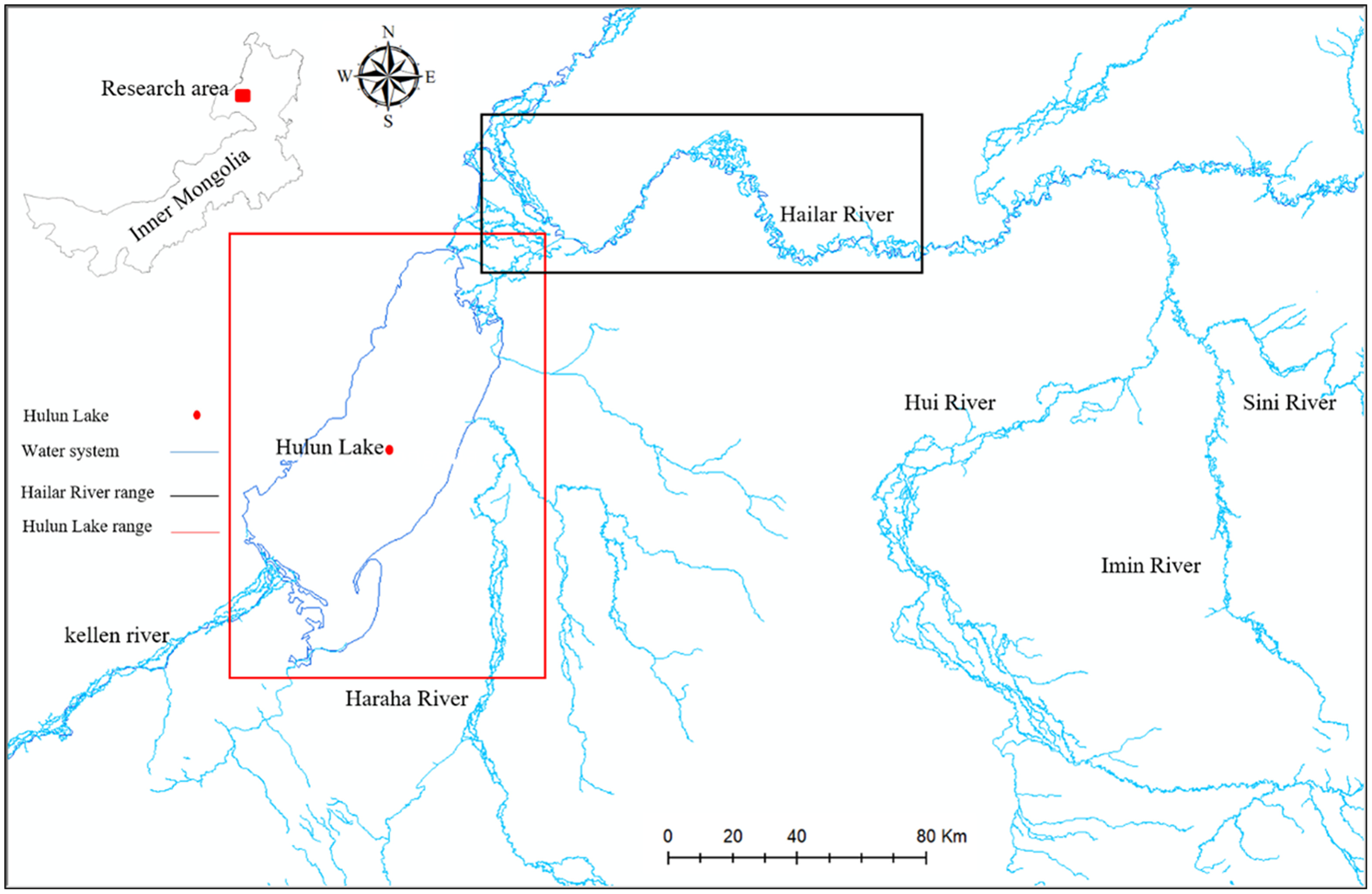
The selected study area contains complex water systems, including Hulun Lake and the lower reaches of Hailar River. Within the area, Hulun Lake has an irregular oblique rectangular surface. The long axis is from southwest to northeast, and the lake is 93 km long and has an area of about . The total area of Hulun Lake and the surrounding wetlands is . The floodplain wetlands and swamps are scattered around Hulun Lake and the Hailar River. When the spring and summer tidal floods arrive, Hulun Lake and the Hailar River easily can spread on both sides, forming wetlands and small lakes with dense tributaries (Cai et al. 2021). The study area has a special position in the protection of the regional ecological environment, playing a very important role in maintaining the biodiversity of the Hulunbuir prairies and the quantity of animal and plant resources.
Data Sources and Processing
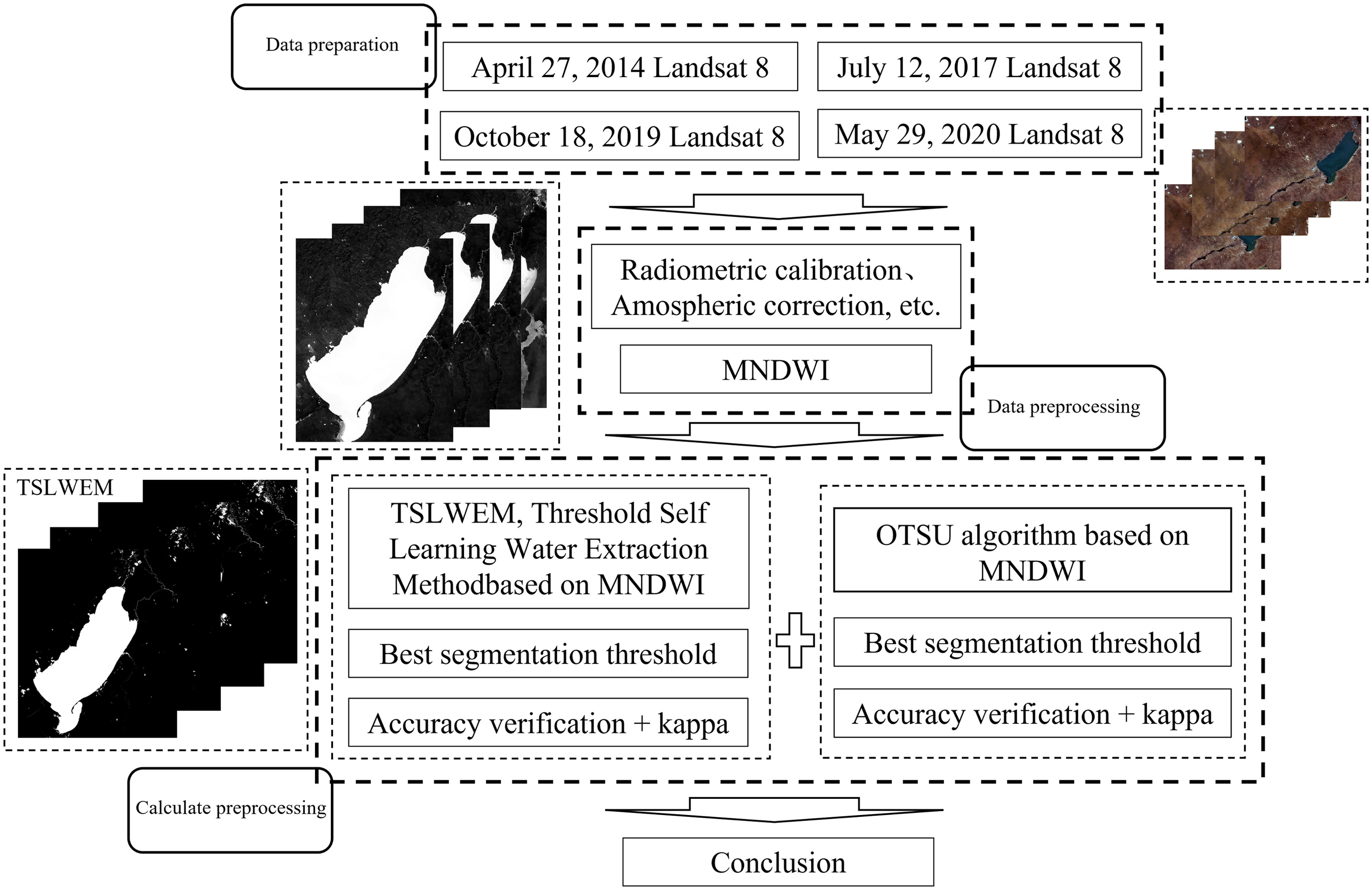
The Landsat 8 Operational Land Imager and Thermal Infrared Sensor (OLI-TIRS) 1T image (Masek et al. 2008) data used in this research were obtained from the National Aeronautics and Space Administration (NASA). This data are presented in Table 1. The image data cover the entire study area. The four selected data periods representing the vegetation phenology (regreening period, maturity period, withering period, and budding period) were April 27, 2014, July 12, 2017, October 17, 2019, and May 29, 2020, respectively. These periods also represented the hydrological seasons, i.e., the spring flood season, summer flood season, dry season, and flatwater season. The water bodies in the study area had various forms (Table 2). This study considered four periods of Landsat 8 data, from 2014 to 2020. According to data records, the lowest water level of Hulun Lake had risen significantly as of May of 2014, and according to the rise of water level, the protection of Hulun Lake has achieved certain results. Therefore, the purpose of selecting this period was to focus on the promotion of the ecological protection on Hulun Lake and its spatiotemporal changes, and on the impact of vegetation around Hulun Lake in different hydrological periods on water extraction. A complex spatial distribution representing different water body conditions and the influence of clouds and weather was considered. The weather was ideal and the data were not disturbed during the data collection. The total cloud amount in the data was less than 2%.
| Satellite | Band | Sensitivity spectrum (μm) | Ground resolution (m) | Nominal spectral location |
|---|---|---|---|---|
| Landsat 8 | 1 | 0.452–0.512 | 30 | Blue |
| 2 | 0.533–0.590 | 30 | Green | |
| 3 | 0.636–0.673 | 30 | Red | |
| 4 | 0.851–0.879 | 30 | Near IR | |
| 5 | 1.566–1.651 | 30 | SWIR-1 | |
| 6 | 2.107–2.294 | 30 | SWIR-2 |
| Data period | Vegetation phenology (Liu et al. 2019) | Hydrological period |
|---|---|---|
| April 27, 2014 | Regreening period | Spring flood season |
| July 12, 2017 | Maturity period | Summer flood season |
| October 18, 2019 | Withering period | Dry season |
| May 29, 2020 | Budding period | Flat water period |
The radiometric calibration tool in ENVI 5.3 was used to calculate the radiometric data, which were input into the FLAASH atmospheric calibration module. The module automatically inputs the corresponding correction parameters from the radiometric image. The atmospheric model was set to the temperate zone (Alexandratos et al. 2019). All reflectance products had values between 0 and 1. Bands 2 and 5 [Green, and shortwave infrared (SWIR)-1] were used. The MNDWI water body index and other parameters were calculated using the band calculation tool.
Research Methods
Determination of the Test Water Body Index
McFeeters (1996) proposed the normalized difference water index (NDWI), but the NDWI considers only the vegetation factor, and ignores the interference of soil and buildings. The spectral characteristics of the latter in green light and the near-infrared (NIR) band are almost the same as those of water, that is, the reflectivity of green light is higher than that in near infrared band, and some of them have large contrast. When extracting water bodies from urban buildings using NDWI, such as water bodies in cities, which leads to confusion between buildings, soil, and water, forming image noise. Xu (2005) based on the theory that the reflection characteristics of the green and near-infrared bands between water and land are similar, and the water in an image often is mixed with the land noise replacing the NIR band with the midinfrared (MIR) band is proposed to realize MNDWI. The calculation model is as follows:where = green band of Landsat 8 OLI data; and = midinfrared band.
(1)
Otsu Algorithm
The Otsu (2007) algorithm assumes that an image contains two types of pixels—foreground pixels and background pixels—in accordance with a bimodal histogram. Therefore, it determines the optimum threshold to separate the two types of pixels in order to minimize their intraclass variance. Because the squared distance between the pairs is constant, their interclass variance is the largest. Using the algorithm [Eq. (2)], the threshold that minimizes the variance within the class is searched thoroughly and defined as the weighted sum of the variances of the two classeswhere = probability that two classes are separated by threshold ; and = variance of two classes.
(2)
The Otsu algorithm proved that minimizing the within-class variance and maximizing the between-class variance were similarwhere = class probability; and = class mean. The class probability () is computed using a histogram with threshold
(3)
(4)
The class mean can be presented aswhere = value of center of th histogram bin. Similarly, () and of the right histogram can be obtained for bins larger than . Class probabilities and class means can be computed iteratively.
(5)
Threshold Self-Learning Water Extraction Method Based on MNDWI
This study proposes a water body extraction method based on the MNDWI water body index with binary segmentation accuracy which can improve water body identification, extract most of the water bodies, reduce the misextraction of other regions, and achieve the optimal segmentation effect. The algorithm has the function of automatically iterating over different segmentation thresholds. The working principle is that the threshold self-learning water extraction method (TSLWEM) algorithm realizes automatic image binary segmentation of the MNDWI water index, that is, the target data are divided into water and nonwater. After the segmentation, the TSLWEM algorithm obtains the segmentation threshold of water and nonwater with different results at the same time. When iterating different segmentation thresholds, the TSLWEM algorithm automatically calculates the accuracy of water extraction under this segmentation threshold, and compares the accuracy of water extraction results with those using other iterative segmentation thresholds. Finally, the threshold with the highest accuracy of water body recognition is determined as the best water body extraction threshold. The workflow of this study is shown in Fig. 2.
The verification data and the interpretation results can be combined to create the following confusion matrix, which is based on the two elements (water and nonwater)
(6)
In the confusion matrix, the behavior interpretation results were listed as verification data and the initial values of , , , and were considered to be zero. Subsequently, the verification data images were traversed while performing threshold verification of the true value points one by one. They then were classified as correct or incorrect. The MNDWI image value range was to 1; therefore, the threshold that affects the segmentation should be as small as possible to ensure that the TSLWEM algorithm can screen any threshold. Therefore the step value was set to 0.0001 and the machine self-learning matrix of the TSLWEM algorithm was obtained using the aforementioned screening of MNDWI images. The confusion matrix iswhere = interpreted to be water, and the verification data are the amount of water (correctly classified as the amount of water); = interpreted to be water, but the verification data are nonwater (wrongly classified as the quantity of water); = interpreted as nonwater, but the verification data are the quantity of water (wrongly classified as nonwater); and = interpreted as nonwater, and the verification data are nonwater (correctly classified as nonwater).
(7)
The calibration process is as follows. After obtaining the confusion matrix of the water and nonwater elements, the TSLWEM algorithm screens the accuracy and kappa coefficient of the confusion matrix, and obtains different water body extraction results using different segmentation thresholds. The TSLWEM algorithm automatically executes the optimal solution of the determination accuracy and kappa coefficient. When the water body extraction accuracy and kappa coefficient are the highest, the result is the best water body extraction result, that is, the threshold of the best segmentation water body.
The overall classification accuracy, known as overall accuracy (OA) (Pekel et al. 2016), is equal to the sum of correctly classified cells divided by the total number of cellswhere = overall classification accuracy.
(8)
The formula for calculating the kappa (Mielke and Berry 2009) coefficient iswhere = overall classification accuracy; and = product of actual and predicted numbers corresponding to all categories, the sum of which is divided by the square of the total number of samples.
(9)
(10)
The verification data contained the field survey of the entire research area conducted in June 2017. A total of 53 sampling points were surveyed, and data such as the coordinates of typical water samples were recorded. The data were based on Google Earth high-resolution images. The area of interest in the real image of the water body was used as a historical data verification sample to extract results of the water body, which consisted of a total of 500 water and nonwater verification samples. The samples consisted of 50 water body sample points and 61 non-water body sample points in April 2014, 82 water body sample points and 65 non-water body sample points in 2017, 46 water body sample points and 63 non-water body sample points in 2019, and 76 water sample points and 57 nonwater sample points of 2020.
Results
Optimal Threshold Determination
The segmentation threshold calculated by the TSLWEM algorithm and that obtained using the Otsu algorithm were compared and analyzed.
The self-iteration of thresholds and accuracy verification and a series of thresholds were tested using the TSLWEM algorithm. The thresholds with the highest water classification accuracy and the best segmentation of water bodies were screened (Table 3). The optimum thresholds of the TSLWEM algorithm were , 0, 0.1990, and on April 27, 2014; July 12, 2017; October 18, 2019; and May 29, 2020, respectively. The optimum thresholds of the Otsu algorithm were 0.1137, 0.1294, 0.1058, and 0.1216 on April 27, 2014; July 12, 2017; October 18, 2019; and May 29, 2020, respectively. The algorithm typically required 10 s to complete a calculation.
| Image acquisition date | Optimal threshold for TSLWEM algorithm | Optimal threshold for Otsu algorithm |
|---|---|---|
| April 27, 2014 | 0.1137 | |
| July 12, 2017 | 0 | 0.1294 |
| October 18, 2019 | 0.1990 | 0.1059 |
| May 29, 2020 | 0.1216 |
Water Body Identification Results
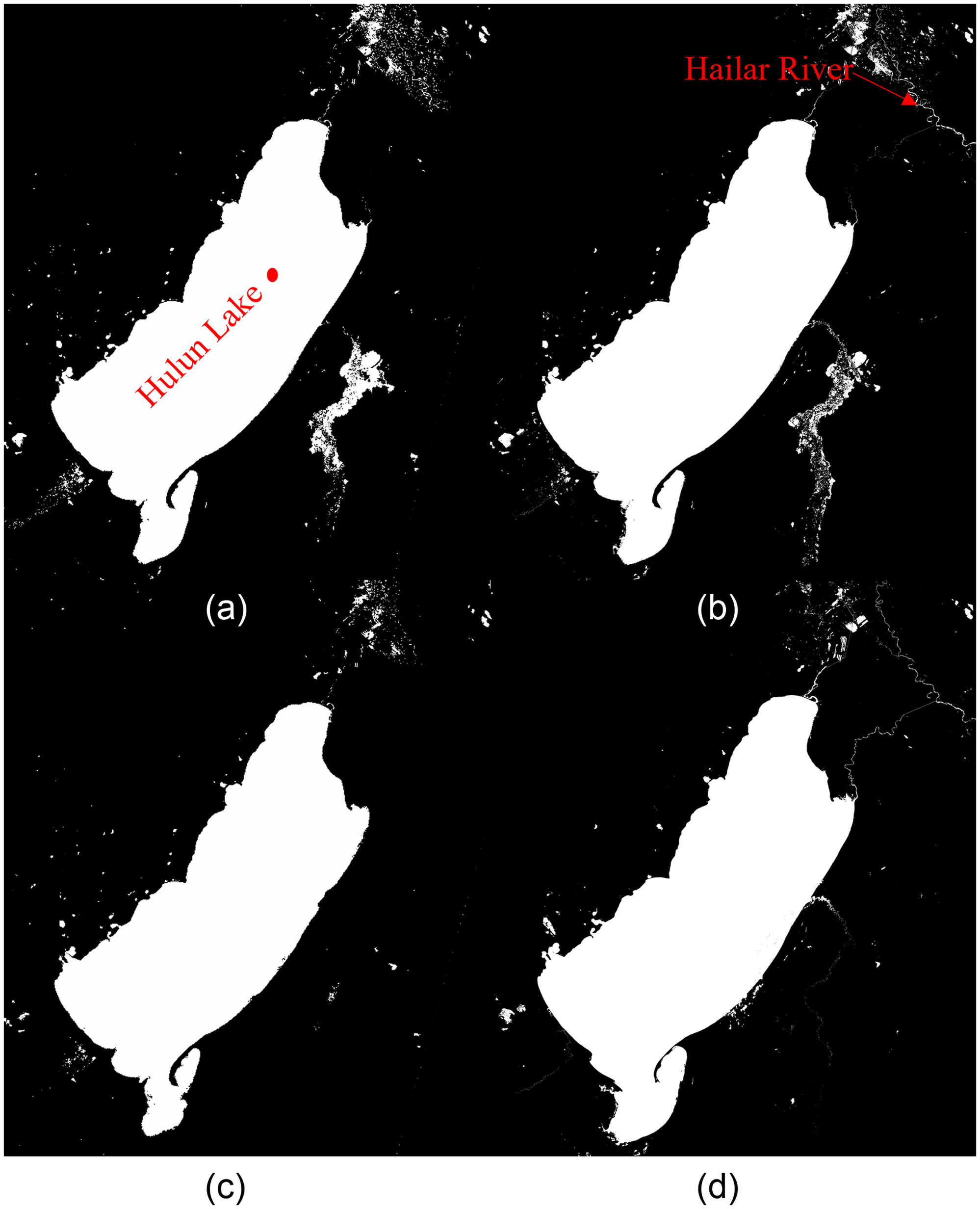
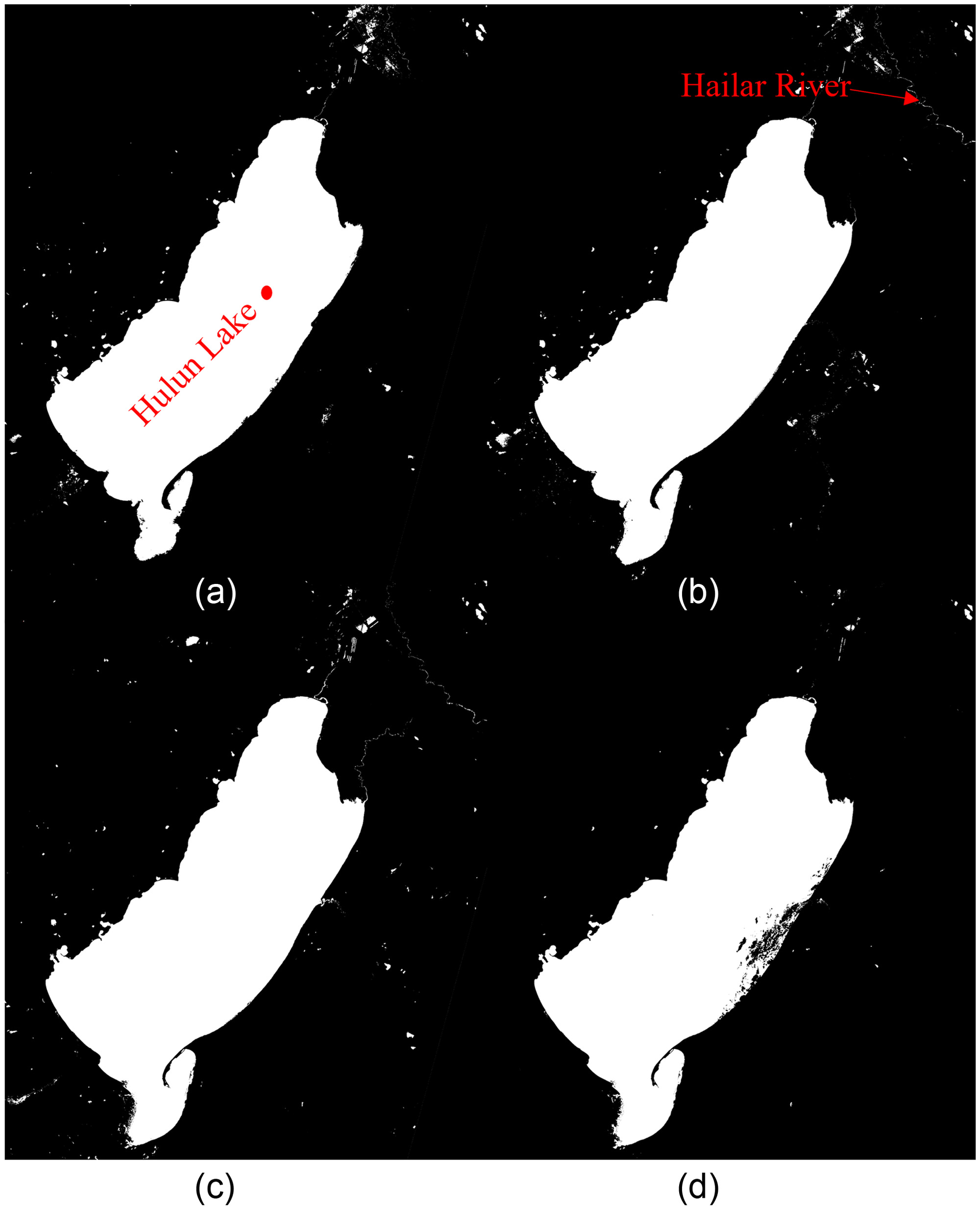
The TSLWEM algorithm extracts the results of water bodies, as shown in Fig. 3. Figs. 3(a and b), and a: show the spring (April 27, 2014) and b show summer (July 12,2017) flood periods of hydrology, respectively. The vegetation is in the green and mature period. The wetland in the southeast of Hulun Lake is full of water, so the target water, lakes, rivers, and small water bodies in the wetland extracted by the TSLWEM algorithm are complete in shape. Figs. 3(c and d) show the normal (October 18, 2019) and dry (May 29, 2020) seasons of hydrology, respectively. During the flowering and dry yellow period of vegetation, there are few water bodies in the wetland in the southeast of Hulun Lake, so the extraction result is different from that in Figs. 3(a and b), and the extraction effect of rivers in the dry season is poor. The OTSU algorithm identified the dry riverbed with high salinity as a water body in the study area (Fig. 4). However, it failed to extract the small water bodies in wetlands [Figs. 3(a and b) and 4(a and b)]. The dry saline-alkali land riverbed, which has a high impact on water body extraction, was eliminated effectively using the grayscale binary image of the water body index of the TSLWEM algorithm. The OTSU algorithm is affected by the complexity of the water body, and the ground features and the water body may be misclassified.
Accuracy Verification
The water classification accuracies of the TSLWEM algorithm and the Otsu algorithm are presented in Table 4. The date with the highest classification accuracy for the TSLWEM algorithm was July 12, 2017. The accuracy of the test data reached 99.93%, with a kappa coefficient of 0.9987 and a water area of . The date with the lowest classification accuracy was May 29 (2020), with a data accuracy of 93.20%, kappa coefficient of 0.8147 and water area of . For the Otsu method, the date with the highest classification accuracy was July 12 (2017), with a water body identification accuracy of 97.24%, kappa coefficient of 0.9173 and the water body area of . The date with the lowest classification accuracy was May 29 (2020) with the water body extraction accuracy of 89.80%, a kappa coefficient of 0.7129 and a water body area of .
| Image acquisition date | Threshold segmentation method | Water area () | Precision (%) | Kappa |
|---|---|---|---|---|
| April 27, 2014 | TSLWEM | 2,162.04 | 98.08 | 0.9426 |
| Otsu | 1,985.56 | 93.32 | 0.7998 | |
| July 12, 2017 | TSLWEM | 2,132.62 | 99.93 | 0.9987 |
| Otsu | 2,024.55 | 97.24 | 0.9173 | |
| October 18, 2019 | TSLWEM | 2,007.00 | 93.39 | 0.8124 |
| Otsu | 2,083.86 | 93.18 | 0.8093 | |
| May 29, 2020 | TSLWEM | 2,130.23 | 93.20 | 0.8147 |
| Otsu | 2,018.09 | 89.80 | 0.7129 |
The aforementioned comparison demonstrated that the accuracy of the TSLWEM algorithm test data exceeded 90%, indicating that the extracted water body results are highly consistent with the verification sample data. The extraction accuracy of the method proposed in this study was significantly higher than that of the OTSU algorithm on the same date. The proposed method highlighted the potential for extracting more accurate water information from Landsat data.
Discussion
Influence of Water Body Index Characteristics on Water Body Extraction
The Otsu algorithm has the advantage of being simple and fast to calculate when extracting water bodies. However, it is sensitive to image noise and can be segmented and extracted only for a single target water body. The intervariance function may exhibit double peaks or multiple peaks. It also is possible that the target water body might not be separated accurately from the background if the grayscale values of the target water body and the background overlap significantly (Li 2022). This might result in a poor extraction effect. This can be attributed to neglecting the spatial information of the image. Additionally, the Otsu algorithm segments the image based on its grayscale distribution, which makes it very sensitive to noise. The TSLWEM algorithm effectively utilizes the threshold distribution of different target objects of the MNDWI water body index and the spatial location information of the target objects.
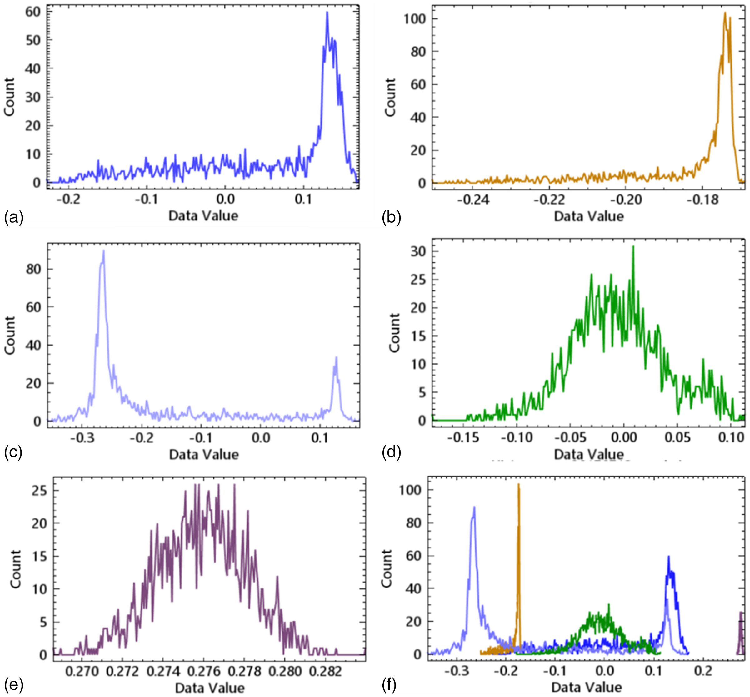
In this study, water in wetlands, dry riverbed, river, vegetation in wetlands, and lake rivers that easily interfere with the results of extraction were selected, using 1,850 sample pixels for each type of surface feature. The average water body index of each surface feature type was calculated (Table 5). The average water body index of lake water was 0.276, and the water body index of each typical surface feature was similar. The mean values of the water body index for each typical feature were found to be similar, other than those for lake water. Similar mean values of water body indexes detrimentally affected water body extraction because the TSLWEM algorithm used different thresholds of water body indexes for image binarization classification.
| Feature type | Average value |
|---|---|
| Water in wetlands | 0.059 |
| River | |
| Lake | 0.276 |
| Dry riverbed | |
| Vegetation in wetlands |
Even if the water was very shallow, the spectral absorption intensity of the water body remained high and the reflected energy was found to be very low for the Landsat 8 OLI water body index image data. A water body’s spectral index differs from those of other ground objects due to its small absorption and high reflection energy (Elsahabi et al. 2016; Feyisa et al. 2014; Wanga et al. 2018). Therefore, using the threshold segmentation method, the threshold range of the spectral index can be used to eliminate the interference of the water body. With the existence of aquatic plants and sediments on the lake surface, the water body index value of a turbid water body could decline, leading to incorrect identification due to the presence of shadows. During the process, wetland water bodies, wetland vegetation, and shallow-water areas near rivers and lakes are prone to misidentification (Gu et al. 2021).
Fig. 5 summarizes the water index distribution characteristics of typical surface features, that is, different surface features that will affect water body identification. The distribution of water body index characteristics of different surface feature types is different. Because there is a large intersection between the threshold distribution range of vegetation in wetlands and water bodies and rivers in wetlands, confusion between these categories will occur during automatic image processing. Therefore, when identifying water bodies in wetlands, the TSLWEM algorithm will extract water bodies by mistake. In addition, the threshold value of lake water is distributed between 0.27 and 0.28, and the threshold value of dry river beds is distributed between and 0.16, which obviously is different from other types of surface objects. Therefore, in the process of automatic extraction of water bodies, these two types of surface objects have less impact on the results of water body extraction during TSLWEM algorithm operation, so the TSLWEM algorithm has obvious advantages in identifying large lakes or distinguishing dry river beds.
Significance and Applicability of the Threshold Self-Adjusting Algorithm in Identifying Water Bodies
This study evaluated the applicability of the proposed TSLWEM algorithm for monitoring and mapping surface water bodies in a temperate semiarid environment using the water body index obtained from Landsat 8 OLI multispectral images. Accurate identification, monitoring, and mapping of water bodies on land surfaces is critical for quantifying and understanding the spatial distribution of water resources and ensuring their sustainable use. Feyisa et al. (2014) introduced a new automatic water extraction index (AWEI) to improve the classification accuracy of areas including shadows and dark surfaces. The AWEI can be used to extract water with high accuracy. Its advantage is that it is applied to the classification error of water bodies caused by shadows in mountainous areas and terrain, which is an important source of classification error. Zhang et al. (2019) used Sentinel-2 images and OpenStreetMap (OSM) data to propose an automatic surface water extraction method based on the presence and background learning algorithm (ASWE-PBL). The research results showed that the ASWE-PBL effectively can suppress the noise caused by shadows and urban areas. Compared with the aforementioned research, the TSLWEM algorithm has a good extraction effect in extracting floodplain wetland and other complex water areas. In our research, we compared only the relative accuracy of the water body results extracted by the TSLWEM algorithm and the Otsu algorithm. Our purpose was to compare the water body extraction accuracy of the two methods in different hydrological phenological periods with a given verification point. Therefore, we did not compare the extraction results with the dynamic surface water range products of Landsat and Moderate Resolution Imaging Spectroradiometer (MODIS) in this research. The extensive application of the TSLWEM algorithm and comparison with existing water extraction products will be our next research focus.
The TSLWEM algorithm proposed in this study was combined with the standard MNDWI water body index. The TSLWEM algorithm employs the threshold difference between the grayscale images of the target water body and other ground object information to remove interference information, and thereby improve the identification accuracy of water bodies. Automatic iterative adjustment, continuous segmentation of the water body with a stepping threshold, and verification of the accuracy of the algorithm were conducted by screening out the best segmentation threshold and obtaining the water body extraction result with the highest classification accuracy. The obtained binarized water body image had a significant effect in suppressing noise, which effectively can reduce the influence of the “same object with a different spectrum, different object with the same spectrum” (Gu et al. 2021). Furthermore, the TSLWEM algorithm uses two-way verification using samples from both water bodies and non-water bodies. To verify the accuracy of the extraction results, the influence of large water body information and the large intersection of the gray values of the vegetation shadow were considered comprehensively when using the spatial location information of the image.
Compared with the Otsu algorithm, the advantages of the TSLWEM algorithm include the accuracy of the water body identification and the automatic iterative verification of the complete threshold (Dong and Hu 2021). The obtained classification results were statistically significant, and the method is universally applicable. The TSLWEM algorithm has higher accuracy and is suitable for extracting surface lake water and river water from complex water bodies. It effectively can eliminate external environmental noise. Therefore, this method was adopted in our study to detect complex surface water information effectively and provide a valuable reference for river management.
Limitations of the Threshold Self-Adjusting Algorithm in Identifying Water Bodies
The TSLWEM algorithm is implemented mostly in a MATLAB environment. The algorithm also can perform operations and implement functions in other environments, including Python, IDL, and R programming languages. This study proved that the proposed TSLWEM algorithm effectively can extract target water bodies from complex semiarid water bodies. Furthermore, in the case of validating samples, the TSLWEM algorithm can be used for other optical satellite sensors, if the provided remote-sensing images have higher resolution. The higher the resolution, the more accurate are the obtained target water data. The use of higher-precision remote-sensing data should be researched in the future.
Our research was limited to specific regions. Water extraction experiments in other regions were not carried out in our research. In the next step, we will focus on the extensive suitability of TSLWEM algorithm in other regions.
To understand the limitations of the TSLWEM algorithm, this study selected four water body test data points in different periods. The following factors affected the algorithm’s ability to extract target water bodies.
1.
Remote-sensing data: This type of data is affected significantly by environmental factors. Limiting environmental factors include atmospheric conditions (clouds and fog), and water clarity and depth. Because the water bodies in the study area are complex, the remote-sensing data could be affected significantly by environmental factors during summer and autumn. The data quality for the summer and autumn seasons was low [Figs. 3(c and d)] (Turlej et al. 2022). Due to these limitations, the verification sample could have difficulty distinguishing between water bodies and non-water bodies, reducing the accuracy of water body identification.
2.
Verify sample data: The TSLWEM algorithm compares any pixel of a water body and a non-water body in the classification result with the verification sample data for the same location. Therefore, the TSLWEM algorithm could be affected significantly by the choice of verification sample. The TSLWEM algorithm will not be able to match the corresponding verification sample data during threshold iteration if the number of verification samples is small or the verification sample points with a low distinction between water bodies and non-water bodies are chosen. As a result, the water body identification accuracy will be reduced.
Conclusion
Based on the MNDWI water body index, this study proposes a new threshold self-learning algorithm to identify water bodies and tested the accuracy of the proposed method in identifying complex water bodies in a specific area. The extraction results of this method demonstrated that the extraction accuracy of the selected test data in the fourth phase exceeded 90%, and the water body accuracy of the test data on July 12, 2017, reached 99.93%. The following conclusions were drawn from the results of this study.
The TSLWEM algorithm effectively can determine the optimal threshold of the grayscale image of the water body index and can distinguish target water bodies from non-water bodies. The recognition accuracy of complex water bodies in large research areas remains difficult when using remote sensing. Compared with traditional methods, the target water bodies obtained by the TSLWEM algorithm are more reliable, and the operation of the algorithm is simple, which has great potential for other optical sensors.
Data Availability Statement
The data set and custom code used or analyzed in the current research can be obtained from the corresponding author upon reasonable request.
Acknowledgments
This work was funded by the National Natural Science Foundation of China (U2102209). Thanks are given to Chunming Hu for proofreading the paper and to Yating Zhao for help with the field experiments.
Author contributions: All authors contributed to the conception and design of this study. Material preparation, data collection and analysis were performed by Xi Dong and Chunming Hu. The first draft of the manuscript was written by Xi Dong. Yating Zhao participated in the collection of verification points, and all authors commented on previous versions of the manuscript. The final manuscript was read and approved by all authors.
References
Abdul Ghofur, M. N., W. S. Udin, H. E. Mansor, and M. M. A. Khan. 2020. “Mapping of groundwater potential zones in a crystalline terrain using remote sensing, GIS techniques and field observations: A case study in parts of Tanah Merah, Kelantan, Malaysia.” IOP Conf. Ser.: Earth Environ. Sci. 549 (Sep): 012026. https://doi.org/10.1088/1755-1315/549/1/012026.
Acharya, T. D., A. Subedi, and D. H. Lee. 2018. “Evaluation of water indices for surface water extraction in a Landsat 8 scene of Nepal.” Sensors 18 (8): 2580. https://doi.org/10.3390/s18082580.
Alexandratos, S. D., N. Barak, D. Bauer, F. T. Davidson, B. R. Gibney, S. S. Hubbard, and P. Westerhof. 2019. “Sustaining water resources: Environmental and economic impact.” ACS Sustainable Chem. Eng. 7 (3): 2879–2888. https://doi.org/10.1021/acssuschemeng.8b05859.
Bhaga, T. D., T. Dube, and C. Shoko. 2020. “Satellite monitoring of surface water variability in the drought prone Western Cape, South Africa.” Phys. Chem. Earth. A/B/C/ 124 (2021): 102914.
Cai, S., X. Song, R. Hu, P. Leng, X. Li, D. Guo, and Y. Wang. 2021. “Spatiotemporal characteristics of agricultural droughts based on soil moisture data in Inner Mongolia from 1981 to 2019.” J. Hydrol. 603 (Jun): 127104. https://doi.org/10.1016/j.jhydrol.2021.127104.
Dong, X., and Z. Chen. 2021. “Digital examination of vegetation changes in river floodplain Wetlands based on remote sensing images: A case study based on the downstream section of Hailar River.” Forests 12 (9): 1206. https://doi.org/10.3390/f12091206.
Dong, X., and C. Hu. 2021. “A new method for describing the inundation status of floodplain wetland.” Ecol. Indic. 131 (10): 108144. https://doi.org/10.1016/j.ecolind.2021.108144.
Elsahabi, M., A. Negm, and A. H. M. H. El Tahan. 2016. “Performances evaluation of surface water areas extraction techniques using Landsat ETM+ data: Case study Aswan High Dam Lake (AHDL).” Procedia Technol. 22 (Jun): 1205–1212. https://doi.org/10.1016/j.protcy.2016.02.001.
Esch, T., V. Himmler, G. Schorcht, M. Thiel, T. Wehrmann, F. Bachofer, C. Bachofer, M. Schmidt, and S. Dech. 2009. “Large-area assessment of impervious surface based on integrated analysis of single-date Landsat-7 images and geospatial vector data.” Remote Sens. Environ. 113 (8): 1678–1690. https://doi.org/10.1016/j.rse.2009.03.012.
Feyisa, G. L., H. Meilby, R. Fensholt, and S. R. Proud. 2014. “Automated water extraction index: A new technique for surface water mapping using Landsat imagery.” Remote Sens. Environ. 140 (9): 23–35. https://doi.org/10.1016/j.rse.2013.08.029.
Gu, Z., Y. Zhang, and H. Fan. 2021. “Mapping inter- and intra-annual dynamics in water surface area of the Tonle Sap Lake with Landsat time-series and water level data.” J. Hydrol. 2021 (1): 126644. https://doi.org/10.1016/j.jhydrol.2021.126644.
Jiang, H., M. Feng, Y. Zhu, N. Lu, J. Huang, and T. Xiao. 2014. “An automated method for extracting rivers and lakes from Landsat imagery.” Remote Sens. 6 (6): 5067–5089.
Khalid, H. W., R. M. Z. Khalil, and M. A. Qureshi. 2021. “Evaluating spectral indices for water bodies extraction in western Tibetan Plateau.” Egypt. J. Remote Sens. Space Sci. 24 (3): 619–634. https://doi.org/10.1016/j.ejrs.2021.09.003.
Li, X., F. Ling, G. M. Foody, D. S. Boyd, L. Jiang, Y. Zhang, and Y. Du. 2021. “Monitoring high spatiotemporal water dynamics by fusing MODIS, Landsat, water occurrence data and DEM.” Remote Sens. Environ. 265 (1): 112680. https://doi.org/10.1016/j.rse.2021.112680.
Li, Y. 2022. “Reservoir water area extraction method.” Comput. Eng. Des. 43 (1).
Liu, Q., S. Piao, Y. H. Fu, M. Gao, J. Peñuelas, and I. A. Janssens. 2019. “Climatic warming increases spatial synchrony in spring vegetation phenology across the Northern Hemisphere.” Geophys. Res. Lett. 46 (3): 1641–1650.
Maliki, A. A. A., A. Chabuk, M. A. Sultan, B. M. Hashim, H. M. Hussein, and N. Al-Ansari. 2020. “Estimation of total dissolved solids in water bodies by spectral indices case study: Shatt al-Arab River.” Water Air Soil Pollut. 231 (9): 1–11. https://doi.org/10.1007/s11270-020-04844-z.
Masek, G. J., C. Huang, R. Wolfe, W. Cohen, F. Hall, J. Kutler, and P. Nelson. 2008. “North American forest disturbance mapped from a decadal Landsat record–ScienceDirect.” Remote Sens. Environ. 112 (6): 2914–2926. https://doi.org/10.1016/j.rse.2008.02.010.
McFeeters, S. K. 1996. “The use of the normalized difference water index (NDWI) in the delineation of open water features.” Int. J. Remote Sens. 17 (7): 1425–1432. https://doi.org/10.1080/01431169608948714.
Mielke, P. W., Jr., and K. J. Berry. 2009. “A note on Cohen’s weighted kappa coefficient of agreement with linear weights.” Stat. Methodol. 6 (5): 439–446. https://doi.org/10.1016/j.stamet.2009.03.002.
Mukherjee, K., and S. Pal. 2020. “Hydrological and landscape dynamics of floodplain wetlands of the Diara region, Eastern India.” Ecol. Indic. 121 (2021): 106961.
Otsu, N. 2007. “A threshold selection method from gray-level histograms.” IEEE Trans. Syst. Man Cyber. 9 (1): 62–66. https://doi.org/10.1109/TSMC.1979.4310076.
Pekel, J. F., A. Cottam, N. Gorelick, and A. S. Belward. 2016. “High-resolution mapping of global surface water and its long-term changes.” Nature 540 (7633): 418–422. https://doi.org/10.1038/nature20584.
Richter, B. D., J. V. Baumgartner, J. Powell, and D. P. Braun. 1996. “A method for assessing hydrologic alteration within ecosystems.” Conserv. Biol. 10 (4): 1163–1174. https://doi.org/10.1046/j.1523-1739.1996.10041163.x.
Rizk, R., M. Alameraw, M. A. Rawash, T. Juzsakova, and K. Rédey. 2021. “Does the Balaton Lake affected by pollution? Assessment through surface water quality monitoring by using different assessment methods.” Saudi J. Biol. Sci. 28 (9): 5250–5260. https://doi.org/10.1016/j.sjbs.2021.05.039.
Shiyan, L., and C. Xiaobin. 2022. “Optimization method for dynamic remote sensing extraction of reservoir water bodies by combining DEM and inundation frequency.” J. Central China Normal Univ. 56 (3): 523–531.
Tri, A., L. Dong, Y. In, and L. Jae. 2016. “Identification of water bodies in a Landsat 8 OLI image using a J48 decision tree.” Sensors 16 (7): 1075. https://doi.org/10.3390/s16071075.
Turlej, C. K., M. Ozdogan, and V. C. Radeloff. 2022. “Mapping forest types over large areas with Landsat imagery partially affected by clouds and SLC gaps.” Int. J. Appl. Earth Obs. Geoinf. 107 (2022): 102689.
Wanga, X., S. Xiea, X. Zhanga, C. Cheng, and G. Hao. 2018. “A robust multi-band water index (MBWI) for automated extraction of surface water from Landsat 8 OLI imagery.” Int. J. Appl. Earth Obs. Geoinf. 68 (19): 73–91. https://doi.org/10.1016/j.jag.2018.01.018.
Xu, H. 2005. “Research on extracting water body information using modified normalized difference water body index (MNDWI).” J. Remote Sens. 10 (5): 589–595.
Yang, F., J. Guo, H. Tan, and J. Wang. 2018. “Automated extraction of urban water bodies from ZY-3 multi-spectral imagery.” Water 9 (2): 144. https://doi.org/10.3390/w9020144.
Yang, K., and L. C. Smith. 2013. “Supraglacial streams on the Greenland ice sheet delineated from combined spectral–shape information in high-resolution satellite imagery.” IEEE Geosci. Remote Sens. Lett. 10 (4): 801–805. https://doi.org/10.1109/LGRS.2012.2224316.
Zhang, Z., X. Zhang, X. Jiang, Q. Xin, Z. Ao, Q. Zuo, and L. Chen. 2019. “Automated surface water extraction combining Sentinel-2 imagery and OpenStreetMap using presence and background learning (PBL) algorithm.” IEEE J. Sel. Top. Appl. Earth Obs. Remote Sens. 12 (10): 3784–3798. https://doi.org/10.1109/JSTARS.2019.2936406.
Information & Authors
Information
Published In

Journal of Hydrologic Engineering
Volume 28 • Issue 8 • August 2023
Copyright
This work is made available under the terms of the Creative Commons Attribution 4.0 International license, https://creativecommons.org/licenses/by/4.0/.
History
Received: Aug 18, 2022
Accepted: Feb 6, 2023
Published online: May 19, 2023
Published in print: Aug 1, 2023
Discussion open until: Oct 19, 2023
ASCE Technical Topics:
- Algorithms
- Aquatic habitats
- Bodies of water (by type)
- Business management
- Ecosystems
- Engineering fundamentals
- Environmental engineering
- Human and behavioral factors
- Lakes
- Mathematics
- Practice and Profession
- River engineering
- Rivers and streams
- Surface water
- Water (by type)
- Water and water resources
- Water management
- Water policy
- Water resources
Authors
Metrics & Citations
Metrics
Citations
Download citation
If you have the appropriate software installed, you can download article citation data to the citation manager of your choice. Simply select your manager software from the list below and click Download.