Investigation on the Water Depth of Choked Flow due to Bottom Blockages in Circular Open Channels
Publication: Journal of Hydraulic Engineering
Volume 150, Issue 5
Abstract
Blockage detection in circular open channels (partially filled pipes, e.g., gravity sewer pipes) has gained increasing interest in the water industry. While there have been significant advancements in monitoring technologies for such systems (e.g., smart sewer systems), there is a lack of quantification of the hydraulic impact of partial blockages in circular pipes, which is a limiting factor for cost-effective detection. This study presents and validates a numerical framework to quantify the changes in water depth caused by extended bottom blockages in circular open channels. The analysis is based primarily on continuity and energy conservation with the assumption of a lossless transition at the blockage. The proposed approach can determine the critical blockage height that would induce choking, therefore a change in the upstream depth. It can also calculate the changed upstream water depth for various bottom blockage height values (above the critical height) for both subcritical and supercritical conditions. The proposed approach is numerically implemented and then validated through a series of laboratory experiments under the subcritical flow condition (which is the most common condition for gravity sewer systems). The numerically determined water depth results are consistent with the experimental results, which confirms that the proposed approach can accurately estimate the new upstream depth under the choking condition induced by a bottom blockage in circular open channels. The results contribute to advancing the hydraulic understanding in circular open channels with extended partial blockages, which is useful in the development of smart sewer technologies.
Practical Applications
Spills and overflows out of the gravity sewer system damage the environment and bring risks to public health. The problem is typically caused by partial blockages, which can reduce the flow capacity of the sewer pipe and induce higher-than-designed flow depth on the upstream of the blockage (known as choked flow condition). This study helps water engineers and operators to understand how an extended bottom blockage affects the flow condition just upstream of the blockage in a circular gravity sewer pipe. Charts have been presented to enable the determination of (1) the critical height of an extended bottom blockage that would induce choking; (2) the expected upstream flow depth for blockages with various heights, with a given flow rate under choked flow condition; and (3) the expected upstream flow depth for various flow rates, with a given blockage height under choked flow condition. The results can be used to evaluate the risk of bottom blockage-induced spill for sewer pipes with various sizes, slopes and flow rates (e.g., some may be more tolerant to bottom blockages while some may be more sensitive). This information can then be used to prioritize preventative measures such as sewer depth monitoring or regular cleaning.
Introduction
Both the water supply and the wastewater collection networks are critical infrastructure for communities. Due to the sheer scale of the pipe networks and the fact that most of them are buried underground, water utilities in most countries are facing challenges in managing aging water and wastewater assets. In the past two decades, substantial research has been conducted for non-destructive and noninvasive defect detection in water networks, such as blockage detection (Duan et al. 2013; Meniconi et al. 2013), leak detection (Covas et al. 2005; Almeida et al. 2018; Wang et al. 2018; Zeng et al. 2020), and pipe condition assessment (Zeng et al. 2018; Zhang et al. 2019; Zeng et al. 2023). The research and development have resulted in the industry application of smart water networks (Rousso et al. 2023). In contrast, research on defect detection in wastewater collection networks (i.e., gravity sewer networks), is very limited. Fundamentals, such as hydraulic modeling (Liu and Chen 2022) and air-water interactions (Qian et al. 2022), are still active research topics for sewer networks.
Sewer blockages pose a serious problem for wastewater network operators since the resultant spills contaminate the environment, endanger public health, and impact the economy (Fenner et al. 2007; DeSilva et al. 2011; Tizmaghz et al. 2022). Consequences of spillages and the costs of excessive preventative maintenance have encouraged innovation directed at developing economical sewer blockage detection techniques (Rodríguez et al. 2012; Mustafa Abro et al. 2019). Advances in sensing and telemetry technology have resulted in an influx of cost-effective devices designed to monitor and report water depths in free-surface flow conditions (Häck and Wiese 2006; Hill et al. 2014). Despite these increasing technological capabilities enabling data-driven and/or threshold analysis of water depths in open channel applications (Edmondson et al. 2018; Webber et al. 2022; Do et al. 2023), the applications are yet to be supported by fundamental knowledge of choking transitions (Henderson 1966) caused by partial blockages.
Transitions and critical flow have traditionally been used for the measurement of flow rate in open channels (Clemmens et al. 2001). For circular open channels, e.g., sewer pipes, Palmer and Bowlus (1936) proposed a Venturi flume with a rectangular or trapezoidal throat for flow measurement. In the short discussion letter on the original paper by Palmer and Bowlus (1936), Stevens (1936) presented a curved slab without any side restrictions (streamlined along the axial direction with no extended flat surface) for flow measurement in sewer pipes. A chart describing the relationship between the depth of approach and the flow rate for a few selected slab heights was provided; however, simplifications were involved in the analysis (a key simplification is that the total energy head at the cross-section corresponding to the highest point of the slab was assumed as the depth of water upstream of the slab for the purposes of calculating the upstream flow area and velocity head). Diskin (1963) developed a pier-shaped structure for flow measurement in sewer pipes. The structure was installed vertically in the center of the channel, and flow was forced to pass through the two sides of the pier-shaped structure where critical flow was established due to the restriction. Wenzel Harry (1975) developed another type of critical flow meter or Venturi flume by introducing one or two smooth and extended restrictions on the sides of the sewer pipe. It could also act as a Venturi meter for full pipe flow. Clemmens et al. (1984) detailed a design of a broad-crested weir for flow measurement in circular pipes flowing partially full. The structure was a horizontal weir sill with a designed length and a ramp at the upstream to minimize energy loss. A table describing the relationship between the specific energy at the upstream of the structure and the flow rate was given. However, the upstream depth was not calculated. Clemmens et al. (1984) stated that an iterative trial-and-error process using two look-up tables could be taken to estimate the upstream depth, which was similar to the approach used in Stevens (1936). Nevertheless, Clemmens et al. (1984) did not follow this approach. Instead, they proposed to use an empirical formula to describe the complex relationship between the flow rate and the upstream depth under choked conditions. The empirical formula was to be calibrated by experimental data.
For circular channels with the channel bed raised due to a change in position of the centerline (the geometry of the cross section does not change), or due to a decrease in channel diameter (the geometry of the cross section is proportionally reduced), Vittal (1978) conducted dimensionless analysis and presented graphical solutions to both choke-free flow and choked flow conditions; Dey (1998) studied the maximum permissible limits of bed elevation rises for choke-free flows and presented graphical solutions; Vatankhah and Bijankhan (2010) further extended the work and provided explicit equations for the maximum allowable bed rise. For circular channels with a bottom blockage (raised channel bed with a flat base but continuous centerline, such that the geometry of the cross section changes with the height of the blockage), most research has focused on sediment transportation (Skipworth Peter et al. 1999; Banasiak and Verhoeven 2008; Seco et al. 2018). Although Dey (1998) analyzed the effect of raised channel bed, which effectively was a partial bottom blockage, the work focused on determining the critical height of the bottom blockage that would just induce critical flow on top of the blockage but no choking to the upstream flow yet, and only the subcritical flow condition was studied. The previous literature review has demonstrated that there is a lack of modern solutions on determining how the height of an extended bottom blockage affects the immediate upstream water depth. This has become a limiting factor for the successful application of smart sewer technologies for blockage detection and spill early warning.
The current research focuses on describing the changes in the hydraulic behavior of circular open channels due to changes in the cross-sectional geometry, with a particular interest on subcritical cases with extended bottom steps to simulate extended bottom blockages (e.g., deposits) in sewer pipes. A numerical framework based primarily on the analysis of the continuity and specific energy conservation was developed to estimate the water depth upstream to a bottom blockage in a circular open channel. The numerical framework extended the analysis by Dey (1998) from choke-free flow to choked flow scenarios for various combinations of blockage, channel and flow conditions. Except for neglecting energy losses, simplifications and empirical analysis used in early studies (Stevens 1936; Clemmens et al. 1984) were avoided in the current work. The numerical solutions for the upstream depth estimation were verified through a controlled set of experiments using a full-scale rig where various conditions (e.g., flow, blockage height, slope) were tested. The numerical solutions can be used for modeling of simple sewer blockages, improving the capability of smart sewer systems for partial blockage detection and sewer spill early warning. Normalized charts describing the relationships are also provided for the ease of practical applications.
Fundamentals of Transitions in Open Channels
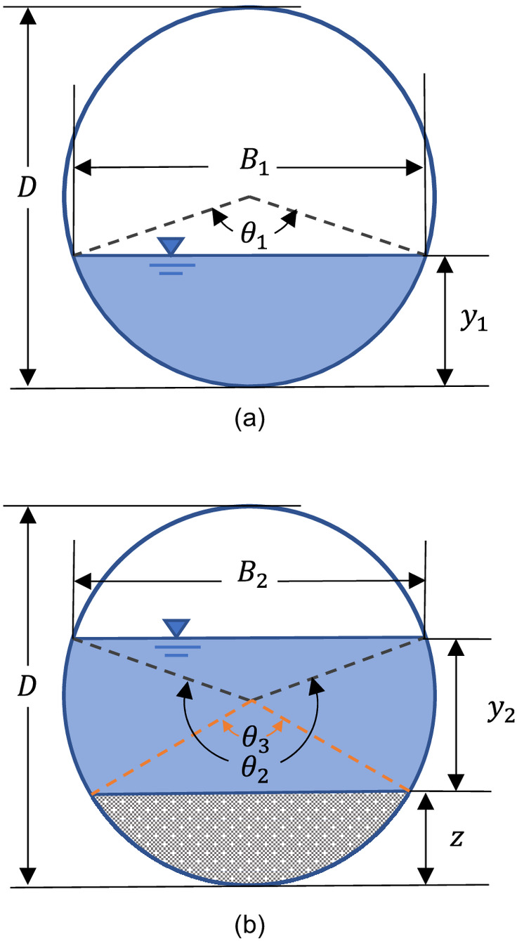
Transition problems are traditionally analyzed using the energy relationship (Chaudhry 2022), where the specific energy is defined aswhere subscript = position in the circular open channel with respect to the blockage (i.e., 1 for upstream and 2 for top of the bottom blockage, used throughout this paper); = depth of water (m); = mean velocity (m/s); and = gravitational acceleration ().
(1)
Neglecting energy losses, upstream () and on top of a bottom blockage () should satisfy , where is the height of the blockage. With increasing from zero, decreases. When is large enough for the flow over the blockage to reach its critical condition, is determined as the critical height of the blockage , where subscript “c” represents the critical flow condition and used throughout this paper. When , the flow over the blockage remains at critical condition such that , and is updated to a new value to satisfy . Depending on the original flow regime (i.e., supercritical or subcritical), may increase or decrease to a new value to match the new energy.
In circular open channels with a bottom blockage, the cross-sectional geometry of the channel changes with . As a result, the curve on top of the blockage changes as a function of for the same . Similarly, the critical flow regime on top of the blockage (i.e., and ) varies with for the same .
Proposed Numerical Framework
A numerical framework is developed to analyze the impact of extended bottom blockage to the upstream flow depth. Energy losses at the transition are neglected, which is applicable to bottom blockages with a smooth ramp on the upstream end (e.g., sediment deposits).
Stage 1: Characterization of the Initial Condition
Analysis of intact and uniform circular open channels, as shown in Fig. 1(a), can be found in the literature (Chaudhry 2022). Assuming known diameter , flow rate and initial water depth upstream to the blockage , the specific energy can be calculated using Eq. (1). For the section upstream of the blockage, it is known thatwhere = wetted area in for the unobstructed section (); and = central angle relative to the water surface (rad, ranging from 0 to ).
(2)
(3)
Eqs. (2) and (3) can be substituted into Eq. (1), resulting in the generic equation to calculate for partially filled unobstructed circular open channels, as shown in Eq. (4)
(4)
Eq. (4) can be normalized by the pipe diameter , and rewritten aswhere , and .
(5)
Changes in and due to downstream blockages are dependent on the original flow regime, determined by the Froude number, as (Chaudhry 2022)where denotes the hydraulic (mean) depth (m). can be calculated aswhere = top width of the flow (m).
(6)
(7)
(8)
Stage 2: Determination of the Critical Blockage Height ()
is defined as the minimum blockage height for a given to give rise to critical flow over the blockage (i.e., , , ). is defined as the minimum specific energy for a given blocked section (i.e., constant , and flow area geometry). Because the geometry of the flow area changes with increases in , as shown in Fig. 1(b), is a function of . The problem is then defined as, for given , and , find the minimum that satisfies
(9)
For a given , can be determined by finding the minimum value in the function, which is given by Eq. (1) and can be rewritten as
(10)
is the flow area at the blocked section, and it can be calculated aswhere = total filled area of the blocked cross section (including flow and blockage) (); is the area of the bottom blockage (); is the central angle relative to the water depth surface on the blocked cross section (rad); and is the central angle relative to the blockage surface (rad). The angles can be calculated by
(11)
(12)
(13)
(14)
(15)
As a result, can be rewritten as
(16)
Similar to the normalization applied to Eq. (4), Eq. (18) can also be normalized by . The normalized blockage height is .
Due to the complexity of the problem and to avoid unrealistic solutions, a three-step numerical procedure for determining was developed. In the first step, is discretized from 0 to with a step size , resulting in a discretized array of . For each realization , the data set are calculated using Eq. (10) and by numerating from 0 to with step size . The minimum value of is found for the particular , and the corresponding is noted as . This should be close to the critical depth for that particular , but not exact due to the discrete step size .
In the second step, for each realization , using as the initial guess, Eq. (17) is solved using iterative nonlinear equation solvers to obtain a more accurate estimation of the critical depth where is the top width of the flow at the blocked section, as shown in Fig. 1(b), given by
(17)
(18)
The corresponding is then determined using and Eq. (10). In the third step, the value of is compared with , with increasing from zero to through the previously discretized array of . It is expected that the value of will increase with increasing values. For the first realization that results in , this is assigned as .
An advantage of this approach is that it is easy to control the system to be always within the free surface flow condition, which is the focus of this research. Another benefit is that the data sets for various blockage height values are readily available and can be used to understand how the curves vary with (as discussed later). Note that there may be other approaches for solving this mathematical problem, but that is not the focus of this research.
Stage 3: Determination of the Condition on top of the Blockage ( and )
The corresponding specific energy on top of the blockage can be calculated by
(19)
For cases where , once is determined using Eq. (19), can be calculated by solving Eq. (10). For cases where , should already be available from the Stage 2 for any discretized .
Note that for some cases (when is relatively large), even though is mathematically possible, it may not be realistic since the flow condition cannot be realized under free surface flow assumption. It is important to check the value of and make sure the value stay less than . When the value is greater than , it indicates that the choking induced by the bottom blockage is so significant such that pressurization of the channel would occur. Analyzing the pressurized condition is out of the scope of this research.
Stage 4: Re-Assessment of the Upstream Condition ( and )
The upstream specific energy remains unchanged if . In contrast, for cases where , the choked flow condition is established, and the upstream specific energy will change to a new value . Provided the critical flow condition can be established on top of the blockage without pressurization, will be the summation of and . The relationships are described by Eq. (20)
(20)
The upstream water depth also remains unchanged for cases where , while it changes for cases where . For the latter, the new upstream water depth can be determined by substituting into Eq. (4) and solving the resulted equation. Care needs to be taken to check whether the determined would result in pressurization of the channel.
Numerical Implementation and Results
Implementation Strategy and Scenarios
The methodology was implemented in R 4.0.4 (R Core Team 2021) using the packages dplyr (Wickham et al. 2021) to pre-process data; nleqslv 3.3.2 (Hasselman 2018) to numerically solve systems of nonlinear equations; and ggplot2 (Wickham 2016) and plotly (Sievert 2020) to visualize solutions. A total of 30 scenarios (Table 1) were simulated for values of , 300 mm, and 600 mm. For , a reference discharge was selected based on the minimum flow required to achieve a velocity of at the typical grade of 1 in 100 for this diameter of circular channel, assuming a Manning’s of 0.013. Based on the , ten values for were chosen to cover a range of typical gravity flow conditions, ranging from 20% to 200% of . For channels with and , the flow rates are chosen to ensure they experience the same normalized flow as for the channel with . For each system (i.e., pairwise and ), and were varied from 0 to with increments of , resulting thus in testing 300,000 cases. However due to extreme variations in the energy-depth relationship close to the bottom and top of the pipe, limits of were applied to ensure meaningful outputs under the free-surface flow condition.
| (mm) | () | () | () | (mm) | (mm) | Step size (mm) |
|---|---|---|---|---|---|---|
| 150 | 1.2 | 12.0 | 1.2 | 15–120 | 0–120 | 1.5 |
| 300 | 6.8 | 68.0 | 6.8 | 30–240 | 0–240 | 3.0 |
| 600 | 38.4 | 384.0 | 38.4 | 60–480 | 0–480 | 6.0 |
Numerical solutions using the package nleqslv 3.3.2 were obtained using a combination of Broyden and Newton methods, described in Dennis and Schnabel (1996). Initial guesses for solving the depth through Eqs. (4) and (10) were chosen within of the corresponding initial condition (i.e., ), based on for the original flow condition.
Numerical Results and Discussion
The methodology enabled the determination of , curves, , and for all cases. As expected, results from the three circular channels with different diameters are consistent after the normalization. Selected results are presented and discussed in the following subsections.
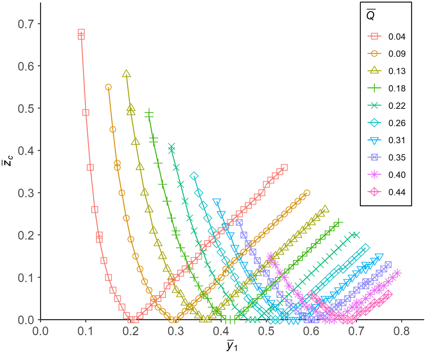
Critical Height of Blockage
Fig. 2 shows the normalized critical height of blockage () for various normalized original flow depths () and normalized flow rates (). The value of firstly decreases with the increase of for all the flows. After reaching zero, the value of then increases with the increase of . The part with the decreasing trend is associated with supercritical flow (), and that with the increasing trend is associated with subcritical flow (). When the original flow condition is critical (), there is no need to have a blockage to induce critical flow, thus the value of is zero. The chart in Fig. 2 can be used by practitioners to estimate the critical bottom blockage height that would induce choking. An example of use is demonstrated in Appendix I.
New Upstream Depth
Fig. 3 shows how the new normalized upstream water depth changes with the normalized block height for various flow rates under the choked flow condition. The upstream water depth response to increasing is dependent on the original flow condition. Expectedly, for cases where and the original flow is subcritical (), increases with increasing , indicating an adjustment in the system’s energy balance by increasing the energy upstream to the blockage. In contrast, for cases where and the original flow is supercritical (), decreases with increasing , indicating an adjustment in the system’s energy balance by increasing the velocity head upstream to the blockage.
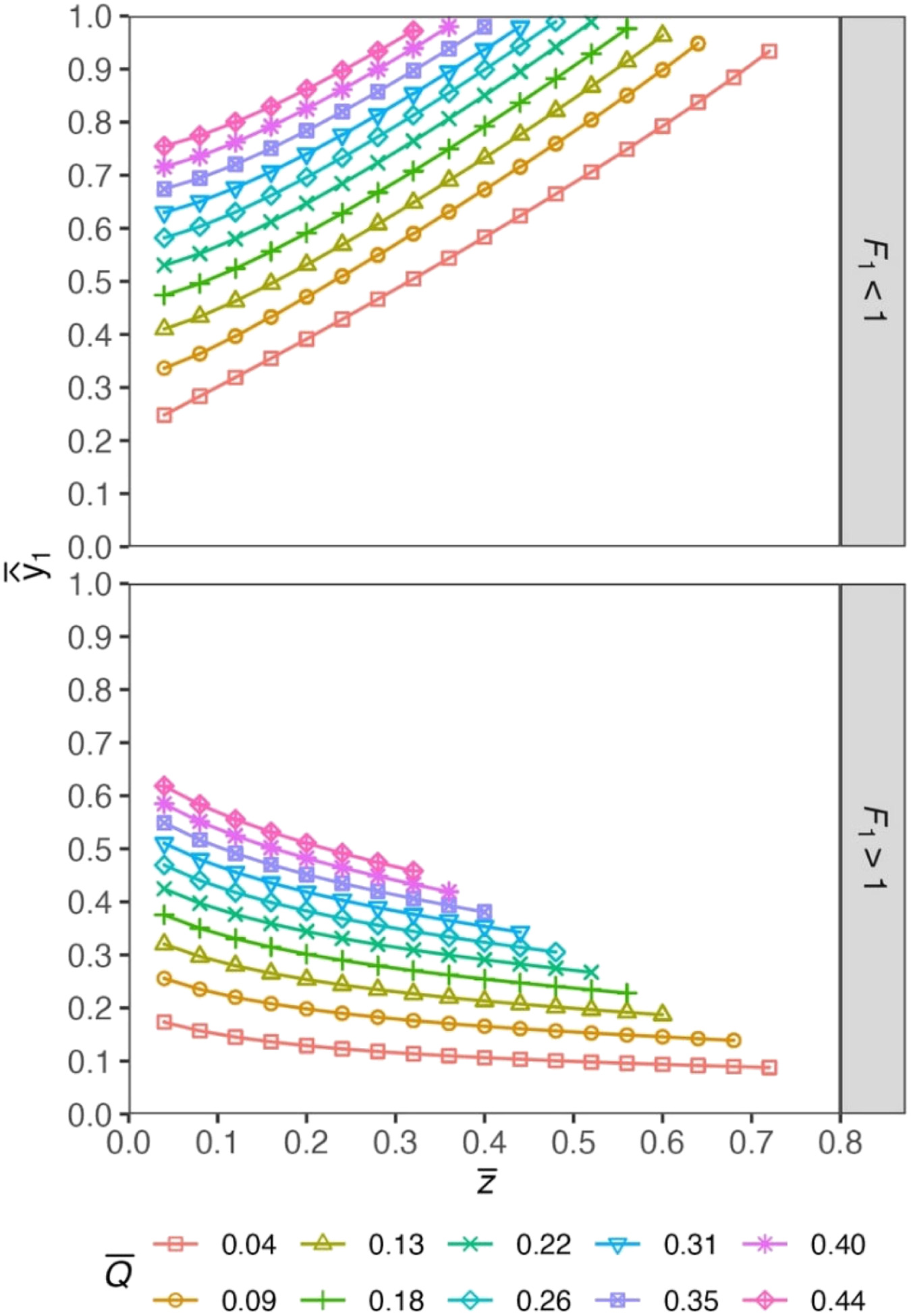
Fig. 4 shows how the new normalized upstream water depth changes with flow rates for various normalized block height values under the choked flow condition. For increasing , increases independently of the original flow regime. However, for increasing for subcritical conditions, the change in is more sensitive to the change in when compared to the supercritical conditions.

The results shown in Figs. 3 and 4 are new contributions made by the current research. Practitioners can use the charts to estimate the new upstream depth for sewer pipes with bottom blockages and experiencing choked flow conditions. An example of use is demonstrated in Appendix I. Most gravity sewer systems are designed to have subcritical flows. For supercritical flows (), it should be noted that there may exist a hysteresis region because of the indeterminable energy losses.
Experimental Validation
Experimental Design and Implementation
Laboratory experiments were conducted to validate the numerical framework and the numerical results by measuring the water depth along a straight section of circular open channels with a bottom blockage. An upstream reservoir supplied a discharge through a 30 m long, 153 mm internal diameter clear PVC pipe. was controlled by adjusting a flow regulation valve in the recirculation line. After any adjustments to the flow regulation valve, the system was left to run for 5 min to reach equilibrium, then was recorded using an ultrasonic flow meter in the recirculation line.
Three blockages were designed and fabricated. Each blockage was designed with a flat top with a length of 700 mm to develop a smooth flow surface through the critical phase, minimizing energy losses due to the transition. The blockages were formed from smooth acrylic with a ramp on the leading edge with a graded entry ramp and graded exit ramp to minimize energy losses and encourage gradual transitions. The height of the three blockages were 40, 50, and 60 mm, respectively.
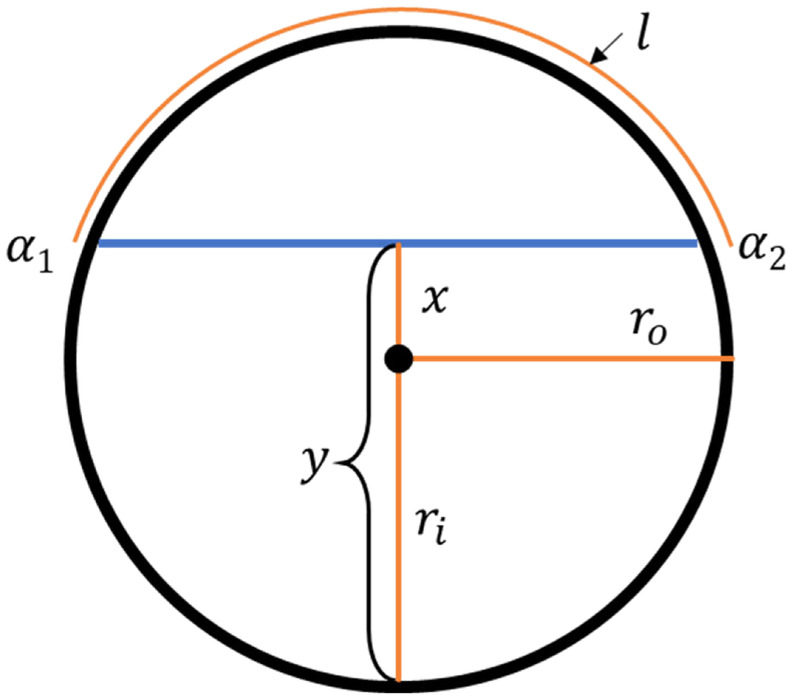
After recording the discharge at the flow meter, the water depth in the clear PVC pipe was measured immediately upstream of the blockage by using measuring bands wrapped around the circumference of the pipe, as shown in Fig. 5. Water depths were calculated by reading the wrapped measuring bands on both sides of the transparent pipe then converting the arclength to water depth (detailed in Appendix II). Precision from reading each band was , which corresponds to an uncertainty about on water depth conversions.

A total of 106 trials were performed by varying and , while and the slope were constant and equal to 153 mm and 0.5%, respectively. was varied from 1 to for the three tested blockages. During all trials the flow regime was subcritical. For each trial, triplicates of and were recorded, while also noting any minor fluctuations () in during pump operations.
Experimental Results and Discussion
Measurements of for the various and tested showed a strong agreement with numerical estimations, as shown in Fig. 6. All increase with increasing and increasing , which is consistent with the normalized numerical results presented in Fig. 4. Discrepancies between numerical estimations and experimental measurements are small (average error of the pipe diameter) and within the reasonable error range. Numerical estimations slightly underestimated experimental measurements for . The experimental results have confirmed that the numerical framework for estimating the impact of a bottom blockage to upstream flow depth are correct.

Conclusion
This study has formulated, implemented, and validated a numerical framework to quantify the water depth in partially filled circular open channels subject to downstream bottom blockages (raised channel bed with a flat base but continuous channel centerline). The numerical estimations of the water depth upstream of the blockage have been validated through a series of experiments using a full-scale setup, showing an excellent agreement between numerical estimations and experimental measurements (average error ).
The proposed numerical framework allows not only the identification of the critical bottom blockage height for any specific circular open channel system, but also a fast and reliable quantification of the new water depth upstream to the bottom blockage for both supercritical and subcritical regimes under choked flow conditions. Graphical solutions have been presented for practitioners to estimate the critical bottom blockage height that would induce choking (Fig. 2), and to determine the new upstream depth under choked but still free-surface flow conditions (Figs. 3 and 4). For systems with subcritical flow regimes, the scenario of particular interest to practitioners managing sewer systems, the upstream water depth proportionally increases with increasing blockage height values and discharge rates. For systems with supercritical flow regimes, the upstream water depth increases with increasing flow rates for a given blockage height but decreases with increasing blockage height for a given flow rate.
This study is limited to free surface flow conditions and bottom blockages. Future work can expand to pressurized conditions and other types and shapes of blockages (i.e., porosity, location in the cross-sectional area of the pipe). The impact of energy losses in supercritical flow conditions also needs further investigation since it might induce hysteresis behavior to the flow depth.
Appendix I. Practical Use of the Normalized Charts
This section demonstrates how the normalized charts presented in Figs. 2–4 can be used to estimate the possible impact of bottom blockages in specific sewer pipe systems. For demonstration, an intact gravity sewer with an internal diameter , a designed dry-weather flow rate of and a corresponding flow depth of is considered. It is also known that the sewer is designed to have subcritical flow, e.g., the corresponding Froude number . Note that all these parameters can be measured from real sewer systems.
The first step is to convert the dimensional flow rate and flow depth to their corresponding normalized values and , and it is achieved by Eqs. (21) and (22)
(21)
(22)
For the specific gravity sewer under consideration, the normalized flow , and the normalized depth . To determine the critical bottom blockage height that would just induce choking, the chart in Fig. 2 is used. The normalized flow is , such that the curve with circular symbols (“o” shaped symbol) should be used (refer to the legend of Fig. 2). Since the normalized depth , based on this value on the x-axis, the corresponding value of the normalized critical blockage height (on the y-axis in the chart) is found to be very close to 0.1 from the curve with circular symbols. Converting this dimensionless height to the corresponding dimensional value by multiplying the diameter, the critical blockage height . This means, for this specific sewer system with the designed flow , a bottom blockage with a heigh of 0.02 m or higher will induce choking.
For a bottom blockage with a heigh of 0.02 m or higher, its impact on the upstream flow depth can be predicted using the charts in Fig. 3. Since the normalized flow is and the flow regime is subcritical (), the curve with circular symbols in the top chart should be used. Note that only the part of the curve with is meaningful. For instance, for a blockage with a height , the corresponding normalized height is . Now referring to the curve with circular symbols in the top chart, the normalized new upstream depth is expected to be . Converting to the corresponding dimensional value, this means the new upstream depth under the choked flow condition is expected to be .
For the same blockage (, ) in the sewer system, its impact under other flow conditions can be assessed using the charts in Fig. 4. Since the flow regime is expected to stay as subcritical, the curve with cross symbols (“+”) in the top chart should be used. For the original designed flow (normalized flow ), the corresponding normalized new upstream depth is read as from the curve. This is consistent with the finding from using Fig. 3. For a higher flow rate, for instance, the corresponding normalized flow is . Using the aforementioned curve, the corresponding normalized new upstream depth can be found by reading the value on the y-axis, and it is . Converting to the corresponding dimensional value, the new upstream depth for the sewer system with a blockage and a flow rate is expected to be .
Appendix II. Conversion of Arclengths to Water Depths
Fig. 7 demonstrates how the water depth can be determined by the arclength. Water depths were calculated by reading the wrapped measuring bands on both sides of the pipe ( and ) and calculating the arclength () of the unfilled section above the flow [Eq. (23)], which was then used to calculate the apothem () while considering pipe wall thickness [Eq. (24)]. Based on , the water depth was estimated by adding or subtracting the apothem to the inside radius, [Eq. (25)]where and are opposite measuring points on the perimeter of the pipe, is the arclength of the section not filled with water, is the apothem, and are respectively the inside and outside radii of the pipe and is the water depth.
(23)
(24)
(25)
Data Availability Statement
The experimental data that support the findings of this study are available from the corresponding author upon reasonable request.
Acknowledgments
The research has been supported by the Barwon Region Water Corporation (Geelong, Australia) and Intelligent Water Networks (https://www.iwn.org.au/) through a collaborative research project (Project Code: PJ06416).
References
Almeida, F. C. L., M. J. Brennan, P. F. Joseph, Y. Gao, and A. T. Paschoalini. 2018. “The effects of resonances on time delay estimation for water leak detection in plastic pipes.” J. Sound Vib. 420 (Apr): 315–329. https://doi.org/10.1016/j.jsv.2017.06.025.
Banasiak, R., and R. Verhoeven. 2008. “Transport of sand and partly cohesive sediments in a circular pipe run partially full.” J. Hydraul. Eng. 134 (2): 216–224. https://doi.org/10.1061/(ASCE)0733-9429(2008)134:2(216).
Chaudhry, M. H. 2022. Open-channel flow. 3rd ed. Cham, Switzerland: Springer.
Clemmens, A. J., M. G. Bos, and J. A. Replogle. 1984. “RBC broad-crested weirs for circular sewers and pipes.” J. Hydrol. 68 (1): 349–368. https://doi.org/10.1016/0022-1694(84)90220-8.
Clemmens, A. J., T. L. Wahl, M. G. Bos, and J. A. Replogle. 2001. Water measurement with flumes and weirs. Wageningen, Netherlands: International Institute for Land Reclamation and Improvement.
Covas, D., H. Ramos, and A. B. De Almeida. 2005. “Standing wave difference method for leak detection in pipeline systems.” J. Hydraul. Eng. 131 (12): 1106–1116. https://doi.org/10.1061/(ASCE)0733-9429(2005)131:12(1106).
Dennis, J. E., Jr., and R. B. Schnabel. 1996. Numerical methods for unconstrained optimization and nonlinear equations. Philadelphia: Society for Industrial and Applied Mathematics.
DeSilva, D., D. Marlow, D. Beale, and D. Marney. 2011. “Sewer blockage management: Australian perspective.” J. Pipeline Syst. Eng. Pract. 2 (4): 139–145. https://doi.org/10.1061/(ASCE)PS.1949-1204.0000084.
Dey, S. 1998. “Choke-free flow in circular channels with increase in bed elevations.” J. Irrig. Drain. Eng. 124 (6): 317–320. https://doi.org/10.1061/(ASCE)0733-9437(1998)124:6(317).
Diskin, M. H. 1963. “Temporary flow measurement in sewers and drains.” J. Hydraul. Div. 89 (4): 141–159. https://doi.org/10.1061/JYCEAJ.0000900.
Do, N. C., L. Dix, M. F. Lambert, and M. L. Stephens. 2023. “Proactive detection of wastewater overflows for smart sanitary sewer systems: Case study in South Australia.” J. Water Resour. Plann. Manage. 149 (1): 05022016. https://doi.org/10.1061/JWRMD5.WRENG-5589.
Duan, H.-F., P. J. Lee, A. Kashima, J. Lu, M. S. Ghidaoui, and Y.-K. Tung. 2013. “Extended blockage detection in pipes using the system frequency response: Analytical analysis and experimental verification.” J. Hydraul. Eng. 139 (7): 763–771. https://doi.org/10.1061/(ASCE)HY.1943-7900.0000736.
Edmondson, V., M. Cerny, M. Lim, B. Gledson, S. Lockley, and J. Woodward. 2018. “A smart sewer asset information model to enable an ‘Internet of Things’ for operational wastewater management.” Autom. Constr. 91 (Jul): 193–205. https://doi.org/10.1016/j.autcon.2018.03.003.
Fenner, R. A., G. McFarland, and O. Thorne. 2007. “Case-based reasoning approach for managing sewerage assets.” Proc. Inst. Civ. Eng. Water Manage. 160 (1): 15–24. https://doi.org/10.1680/wama.2007.160.1.15.
Häck, M., and J. Wiese. 2006. “Trends in instrumentation, control and automation and the consequences on urban water systems.” Water Sci. Technol. 54 (11–12): 265–272. https://doi.org/10.2166/wst.2006.797.
Hasselman, B. 2018. “nleqslv: Solve systems of nonlinear equations.” In R package version 3.3.2. Vienna, Austria: R Foundation for Statistical Computing.
Henderson, F. M. 1966. Open channel flow. New York: Macmillan.
Hill, D., B. Kerkez, A. Rasekh, A. Ostfeld, B. Minsker, and M. K. Banks. 2014. “Sensing and cyberinfrastructure for smarter water management: The promise and challenge of ubiquity.” J. Water Resour. Plann. Manage. 140 (7): 01814002. https://doi.org/10.1061/(ASCE)WR.1943-5452.0000449.
Liu, X., and S. Chen. 2022. “Improved modeling of flows in sewer pipes with a novel, well-balanced MUSCL scheme.” J. Hydraul. Eng. 148 (12): 04022024. https://doi.org/10.1061/(ASCE)HY.1943-7900.0002011.
Meniconi, S., H. F. Duan, P. J. Lee, B. Brunone, M. S. Ghidaoui, and M. Ferrante. 2013. “Experimental investigation of coupled frequency and time-domain transient test-based techniques for partial blockage detection in pipelines.” J. Hydraul. Eng. 139 (10): 1033–1040. https://doi.org/10.1061/(ASCE)HY.1943-7900.0000768.
Mustafa Abro, G. E., B. Jabeen, K. K. Ajodhia, A. Rauf, A. Noman, S. F. ul Huda, and A. AliQureshi. 2019. “Designing smart sewerbot for the identification of sewer defects and blockages.” Int. J. Adv. Comput. Sci. Appl. 10 (2): 615–619. https://doi.org/10.14569/IJACSA.2019.0100276.
Palmer, H. K., and F. D. Bowlus. 1936. “Adaptation of Venturi flumes to flow measurements in conduits.” Trans. Am. Soc. Civ. Eng. 101 (1): 1195–1216. https://doi.org/10.1061/TACEAT.0004761.
Qian, Y., Z. Zhu David, and B. van Duin. 2022. “Design considerations for high-speed flow in sewer systems.” J. Hydraul. Eng. 148 (9): 03122001. https://doi.org/10.1061/(ASCE)HY.1943-7900.0002004.
R Core Team. 2021. R: A language and environment for statistical computing. Vienna, Austria: R Foundation for Statistical Computing.
Rodríguez, J. P., N. McIntyre, M. Díaz-Granados, and Č. Maksimović. 2012. “A database and model to support proactive management of sediment-related sewer blockages.” Water Res. 46 (15): 4571–4586. https://doi.org/10.1016/j.watres.2012.06.037.
Rousso, B. Z., M. Lambert, and J. Gong. 2023. “Smart water networks: A systematic review of applications using high-frequency pressure and acoustic sensors in real water distribution systems.” J. Cleaner Prod. 410 (Jul): 137193. https://doi.org/10.1016/j.jclepro.2023.137193.
Seco, I., A. Schellart, M. Gomez-Valentin, and S. Tait. 2018. “Prediction of organic combined sewer sediment release and transport.” J. Hydraul. Eng. 144 (3): 04018003. https://doi.org/10.1061/(ASCE)HY.1943-7900.0001422.
Sievert, C. 2020. Interactive Web-Based Data Visualization with R, plotly, and shiny. Boca Raton, FL: CRC Press.
Skipworth Peter, J., J. Tait Simon, and J. Saul Adrian. 1999. “Erosion of sediment beds in sewers: Model development.” J. Environ. Eng. 125 (6): 566–573. https://doi.org/10.1061/(ASCE)0733-9372(1999)125:6(566).
Stevens, J. C. 1936. “Adaptation of Venturi flumes to flow measurements in conduits.” Trans. Am. Soc. Civ. Eng. 101 (1): 1217–1235. https://doi.org/10.1061/TACEAT.0004742.
Tizmaghz, Z., J. E. Van Zyl, and T. F. P. Henning. 2022. “Consistent classification system for sewer pipe deterioration and asset management.” J. Water Resour. Plann. Manage. 148 (5): 04022011. https://doi.org/10.1061/(ASCE)WR.1943-5452.0001545.
Vatankhah, A. R., and M. Bijankhan. 2010. “Choke-free flow in circular and ovoidal channels.” Proc. Inst. Civ. Eng. Water Manage. 163 (4): 207–215. https://doi.org/10.1680/wama.2010.163.4.207.
Vittal, N. 1978. “Direct solution to problems of open channel transitions.” J. Hydraul. Div. 104 (11): 1485–1494. https://doi.org/10.1061/JYCEAJ.0005097.
Wang, X., D. P. Palomar, L. Zhao, M. S. Ghidaoui, and R. D. Murch. 2018. “Spectral-based methods for pipeline leakage localization.” J. Hydraul. Eng. 145 (3): 04018089. https://doi.org/10.1061/(ASCE)HY.1943-7900.0001572.
Webber, J. L., T. Fletcher, R. Farmani, D. Butler, and P. Melville-Shreeve. 2022. “Moving to a future of smart stormwater management: A review and framework for terminology, research, and future perspectives.” Water Res. 218 (Jun): 118409. https://doi.org/10.1016/j.watres.2022.118409.
Wenzel Harry, G. 1975. “Meter for sewer flow measurement.” J. Hydraul. Div. 101 (1): 115–133. https://doi.org/10.1061/JYCEAJ.0004159.
Wickham, H. 2016. ggplot2: Elegant graphics for data analysis. New York: Springer.
Wickham, H., R. François, L. Henry, and K. Müller. 2021. “dplyr: A grammar of data manipulation.” In R package version 3.3.2. Vienna, Austria: R Foundation for Statistical Computing.
Zeng, W., J. Gong, P. R. Cook, J. W. Arkwright, A. R. Simpson, B. S. Cazzolato, A. C. Zecchin, and M. F. Lambert. 2020. “Leak detection for pipelines using in-pipe optical fiber pressure sensors and a paired-IRF technique.” J. Hydraul. Eng. 146 (10): 06020013. https://doi.org/10.1061/(ASCE)HY.1943-7900.0001812.
Zeng, W., J. Gong, A. C. Zecchin, M. F. Lambert, B. S. Cazzolato, and A. R. Simpson. 2023. “Reconstructing extended irregular anomalies in pipelines using layer-peeling with optimization.” J. Hydraul. Eng. 149 (1): 04022035. https://doi.org/10.1061/JHEND8.HYENG-13106.
Zeng, W., J. Gong, A. C. Zecchin, M. F. Lambert, A. R. Simpson, and B. S. Cazzolato. 2018. “Condition assessment of water pipelines using a modified layer peeling method.” J. Hydraul. Eng. 144 (12): 04018076. https://doi.org/10.1061/(ASCE)HY.1943-7900.0001547.
Zhang, C., J. Gong, A. Simpson, A. Zecchin, and M. Lambert. 2019. “Impedance estimation along pipelines by generalized reconstructive Method of Characteristics for pipeline condition assessment.” J. Hydraul. Eng. 145 (4): 04019010. https://doi.org/10.1061/(ASCE)HY.1943-7900.0001580.
Information & Authors
Information
Published In

Journal of Hydraulic Engineering
Volume 150 • Issue 5 • September 2024
Copyright
This work is made available under the terms of the Creative Commons Attribution 4.0 International license, https://creativecommons.org/licenses/by/4.0/.
History
Received: Sep 8, 2023
Accepted: Feb 19, 2024
Published online: Jun 12, 2024
Published in print: Sep 1, 2024
Discussion open until: Nov 12, 2024
Authors
Metrics & Citations
Metrics
Citations
Download citation
If you have the appropriate software installed, you can download article citation data to the citation manager of your choice. Simply select your manager software from the list below and click Download.