Impact of Filter Unit Placement on Suspended Sediment Deposition Promotion in Rivers
Publication: Journal of Hydraulic Engineering
Volume 150, Issue 6
Abstract
A filter unit (FU) is a structure installed with the aim of protecting the foundation of an embankment revetment from riverbed scouring, and there are cases in which sediment is deposited in the surrounding area after installation. Vegetation growth in sediment can improve the environment and protect revetments. Hydraulic experiments and numerical calculations were conducted to investigate how suspended sediments are deposited around FUs over a large area within a short period of time. We performed suspended sediment deposition experiments using FU models and confirmed that sediment deposition can be calculated accurately using a two-dimensional planar model. We also analyzed FU placement and its impact on topographical changes in an actual river in which FUs were installed. The results showed that (1) the continuous placement of FUs inhibits sediment deposition on the downstream side; (2) arranging FUs at intervals facilitates sediment deposition even under small-scale floods; and (3) employing an interval of half the FU width for every three or more FUs can effectively promote suspended sediment deposition at intervals.
Introduction
Foot protection work is engineered with the aim of protecting the foundation of river structures such as embankment revetments and bridge piers from riverbed scouring, and commonly is used in conjunction with toe protection. There is a need for designs and materials that consider the river environment. A filter unit (FU) is a structure in which natural stones with a grain size ranging from 50 to 200 mm are packed in a bag-shaped 25-mm synthetic fiber mesh. Crushed concrete also can be used instead of natural stone. The FU has a cylindrical shape, and the size ranges from a 1-t type to a 4-t type, and is determined according to the design flow velocity of the river. The FU is used as a foot protection structure with a minimal environmental load due to its adoption of naturally derived materials and presence of many voids, which can provide habitats for living organisms (Mohamed 2010). There have been several cases of sediment deposition in areas surrounding FUs following their installation, and vegetation could grow in the deposited sediment. It is widely accepted that vegetation growing in riverbanks reduces the fluid forces acting on revetments (Ikeda and Izumi 1990; Ali and Uijttewaal 2013). Additionally, the vegetation occurring around the bridge pier reduces surrounding riverbed scouring (Yoon and Kim 2005). Although riverbed scouring can cause the outflow of vegetated soil (Fukuoka et al. 1998), vegetation at a FU site will not flow away unless the FU itself is moved by flooding. Although riverbank vegetation can narrow the river channel and increase the water level, if vegetation grows only in FUs, the vegetation area can be limited.
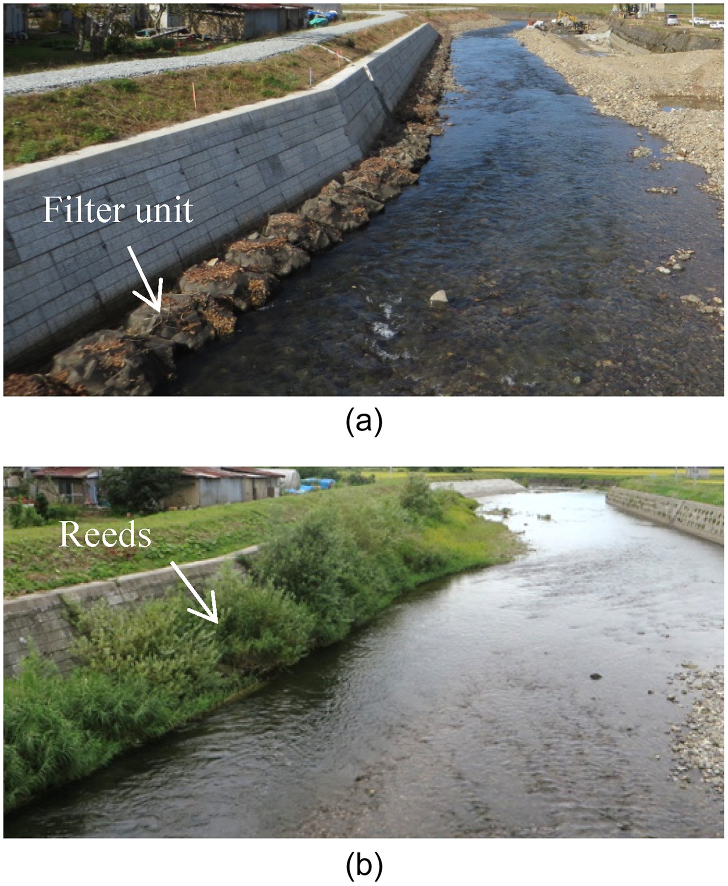
The authors conducted a follow-up survey of FUs installed in the Babame River, Akita Prefecture, Japan. Three years after installation, fine sediment deposition was observed around the installed FUs, and 6 years after installation mainly reed vegetation occurred, growing to over 2 m (Fig. 1). Small fish with body lengths of approximately 0.05 m were observed near the vegetation, confirming that the installed FUs can serve as a habitat for living organisms. During this period, there was a flood that exceeded the design flow rate before vegetation growth, and a disaster occurred in which the slope of an embankment collapsed within the FU installation range. There is a possibility that the damage could have been mitigated had vegetation grown sufficiently before the flood. Consequently, sediment deposition over a large area around the FUs within a short period could be important in terms of the environment and protection of river structures. The provision of foot protection at intervals could create various environments and affect sediment deposition (Hagiwara et al. 2020). However, no attention has been given to sedimentation in foot protection work overall, including FUs.
In contrast to foot protection work, groin work involves a structure that reduces river flow and protects embankments. The shape and arrangement of groins that promote sediment deposition have been studied using experiments and numerical simulations (Alauddin and Tsujimoto 2012; Kyuka et al. 2016; Giglou et al. 2018). Although the flow around groins is complex, the area in which the flow has a strong three-dimensionality is limited. Tingsanchali and Maheswaran (1990) analyzed the flow around an impermeable groin using a depth-averaged two-dimensional model and showed that the surrounding flow could be reproduced with high accuracy, except for the tip of the groin. Regarding permeable groins, surrounding flow and riverbed fluctuation have been captured using two-dimensional models (Ikeda et al. 1991; Ezzeldin 2019). In addition to the groins, the flow around continuously placed rectangular blocks has been calculated using a two-dimensional model (Fukuoka et al. 1999). Even around continuously placed FUs, three-dimensional complex flows are limited to areas with sudden flow changes, such as the upstream end, and the surrounding flow and riverbed fluctuation can be calculated using a two-dimensional model. However, verifying the accuracy of numerical models is difficult due to the lack of research examples of sediment deposition around foot protection works, including FUs.
Therefore, this study verified the model accuracy by investigating sediment deposition around FUs in hydraulic experiments and by comparing the experimental results to numerical simulations. We show that the sedimentation around the installed FUs can be reproduced using a two-dimensional model, but validation was insufficient (Hagiwara et al. 2022b). The present paper improved the accuracy of sedimentation calculation and validated the numerical model. Furthermore, we performed numerical simulations of the actual Babame River and investigated methods for promoting suspended sediment deposition around FUs.
Methods
Target Area
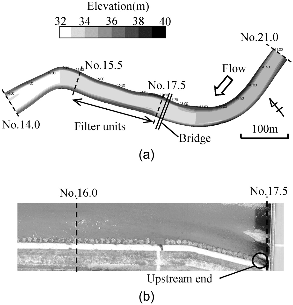
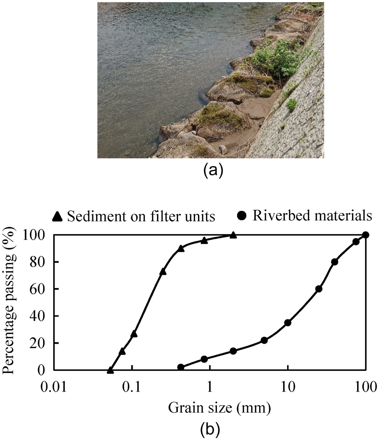
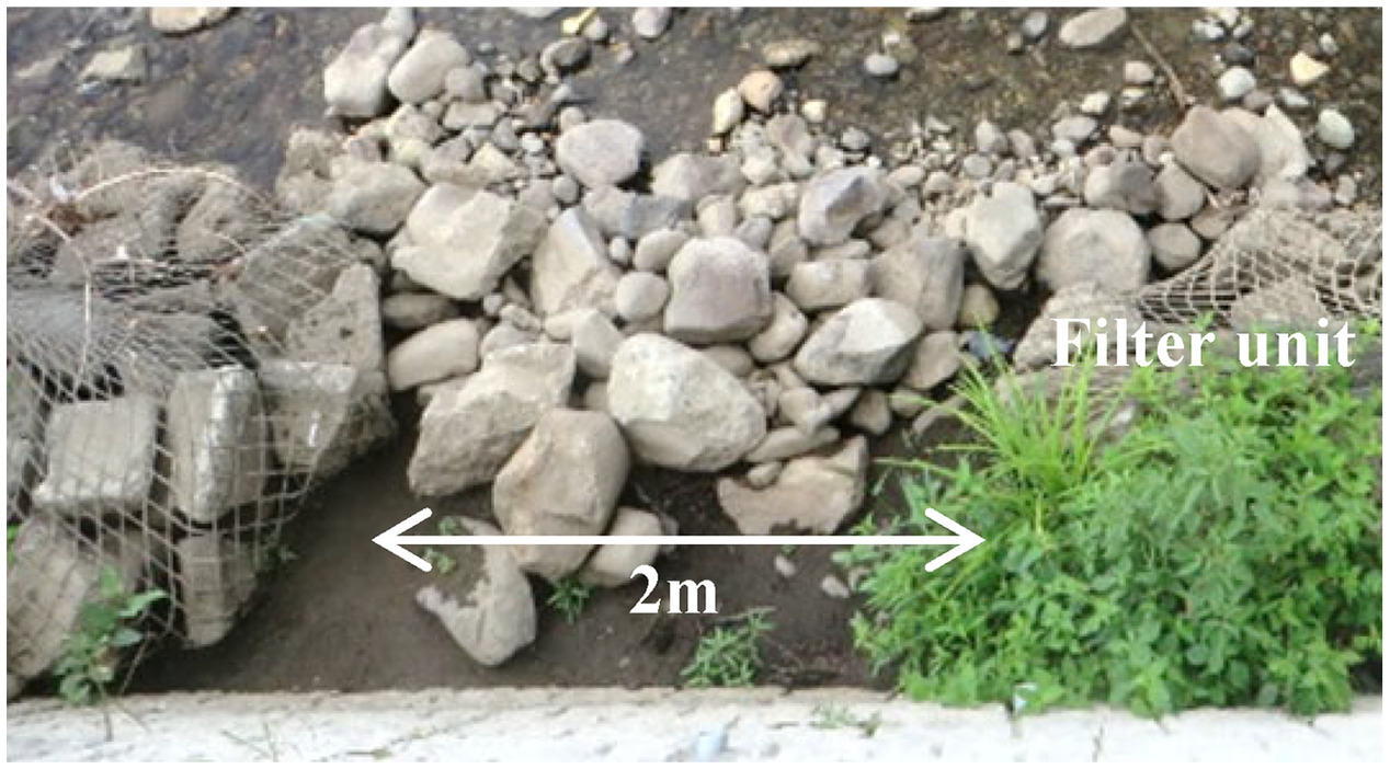
The analysis target is a section with a length of approximately 700 m of the Babame River in Akita Prefecture, located at latitude 39.90° north and longitude 140.18° east, ranging from Section No. 14.0 from Section No. 21.0 [Fig. 2(a)]. The Babame River is a medium-sized river with a basin area of . The target site is located approximately 15 km upstream from the river mouth, and the bed slope is 1/500. Here, the average width of the river and the embankment height are approximately 40 and 4 m, respectively. Normally, the flow rate is so low that part of the riverbed is exposed, but during the flood season, the water level can exceed the embankment. In 2015, a row of 2-t-type FUs (cylindrical, with a weight of 2 t, a diameter of 1.9 m, and a height of 0.4 m) were installed in the section extending from No. 15.5 to No. 17.5 on the left bank of the river [Fig. 2(b)]. Sediment deposition and vegetation growth around the FUs were confirmed in 2021 [Fig. 1(b)]. Deposition was prominent around the FUs on the upstream side, and sediment was deposited inside and on the FUs and within the gaps between the FUs [Fig. 3(a)]. Fig. 3(b) shows the grain size of the riverbed material and sediment deposited on the FUs. Both materials were collected in November 2020. The grain size of the riverbed material ranged from 0.2 to 100 mm, with a median diameter of 15 mm, whereas the sediment on the FUs ranged from 0.02 to 2 mm in size, with a median diameter of 0.2 mm. Because the grain-size distributions differed by more than 80%, we hypothesized that the sediment originated from the upstream side during floods.
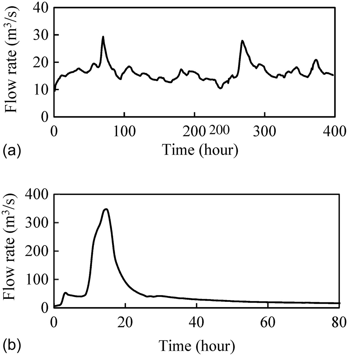
The annual flood pattern is regular overall, with a low flow rate (less than ) in winter when snow accumulates, an increase in the flow rate () during the snowmelt season from March to April, and several floods due to rainfall in summer. It is assumed that sediment deposition progresses during the FU submerged period, such as snowmelt floods and summer floods (Tanaka et al. 2014). When the authors sampled and analyzed river water during small-scale summer floods (a flow rate of ), the suspended sediment concentration was , and the median grain size was 0.04 mm, which is within the range of the observation data for Japanese rivers (Kawamura et al. 1997).
Experimental Methods
A hydraulic model experiment was conducted to obtain the sedimentation tendency around FUs and validate the applicability of the numerical model. Here, the reproduction of the target river was not the purpose. The experimental equipment used included a gradient slope open channel with a width of 0.4 m, depth of 0.5 m, and length of 20 m. A 2-m section at the upstream end was covered with sand (0.05 m thick), and a constant flow was applied to generate suspended sediment [Figs. 4(a and b)]. The channel floor was constructed of mortar, and the bed slope was 1/500. The sand used was quartz sand, with a grain size ranging from 0.05 to 0.2 mm and a median grain size of 0.1 mm.
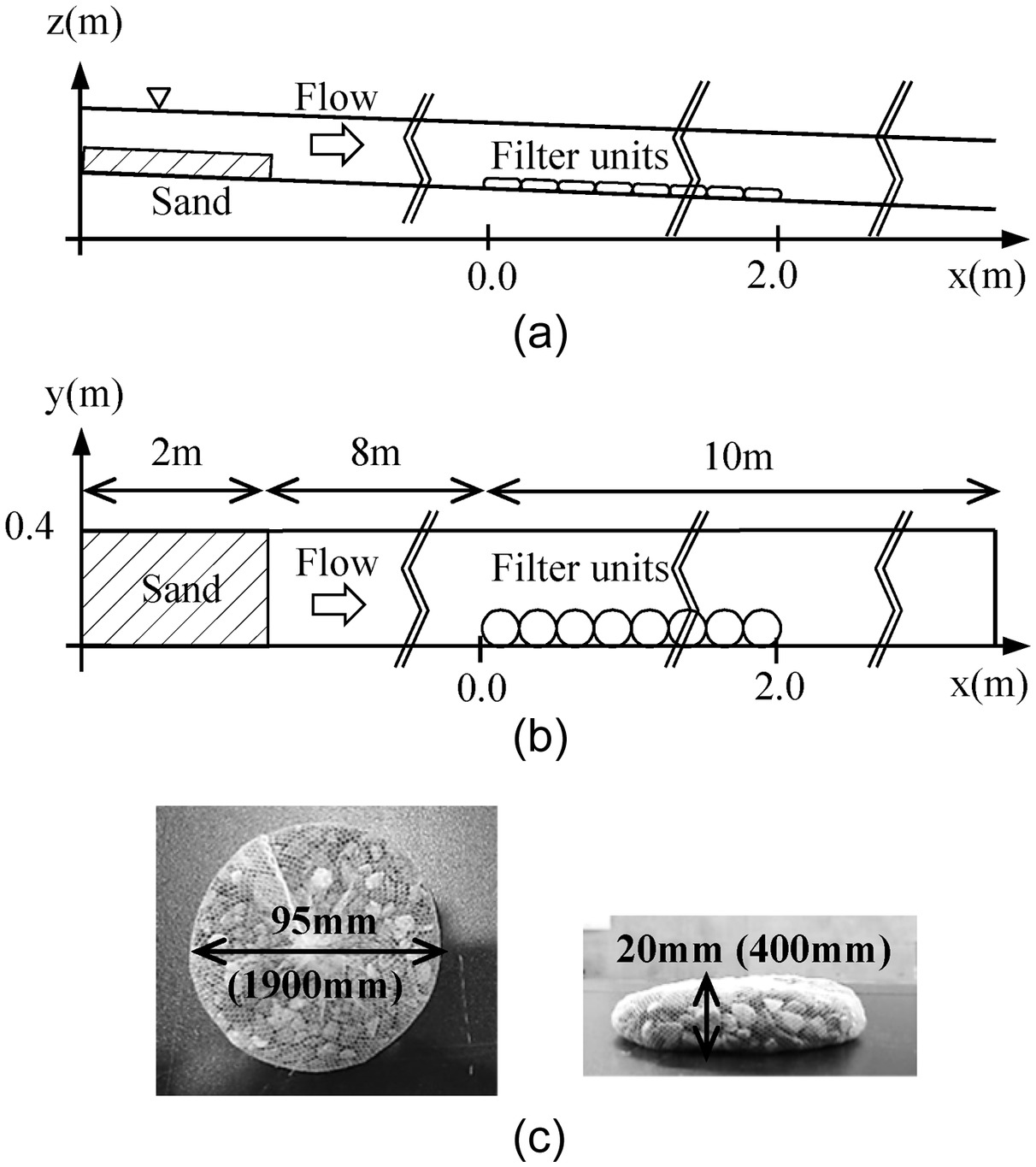
For the experiment, we prepared 1/20-scale models of the 2-t-type FU, which were filled with pebbles in 1-mm mesh material [Fig. 4(c)]. The grain size of the internal pebbles was approximately 5 mm (50–20 mm in the prototype), and the specific weight was 2.65, the same as the prototype. The weight of the FU model was 0.25 kg, which corresponds to 2 t of the prototype based on Froude’s similarity. The FU models were arranged in a single row from on the right bank of the channel. The experimental flow rate was set to , which corresponds to in the Babame River based on Froude’s similarity law and considering the river width. The experimental flow rate targeted a flow rate of , which is the flow rate during the snowmelt flood or decay period of summer floods of the target river. The downstream end of the channel exhibited free flow without adjusting the water depth.
The experiment was repeated two times under the same conditions. To start the experiment, the sand and FU models were set at predetermined positions, and the flow rate was adjusted by opening the valve to achieve the target flow rate. At first, water flowed over the sand layer, after which the sand layer gradually collapsed, becoming a muddy stream flowing downstream. The muddy stream persisted until the suspended sediment settled and topographic change subsided, after which the flow was stopped to end the experiment. After the experiment, the deposited sand and FU models were removed and again placed at predetermined positions, and the experiment was repeated. In the experiment, the sediment thickness, flow velocity, and water depth around the FU were measured. The sediment thickness was analyzed using photographs obtained from the side of the channel. At several points along the FU and at the center of the channel, the flow velocity was measured at 0.1-s intervals with an electromagnetic current meter (KENEK VM801H, Tokyo) without suspended sediment. The water depth was measured with a point gauge.
Calculation Methods
Nays2DH version 3.0 river simulation software was used to model the flow and riverbed fluctuation around the FUs; Nays2DH was developed in Japan and can be applied worldwide (Shimizu et al. 2014). It was verified that this model suitably represents the experimental flow and riverbed fluctuation values around groins (Alauddin and Tsujimoto 2012; Ezzeldin 2019). Eq. (1) is the continuity equation and Eqs. (2) and (3) are the equations of motion of the flow for riverbed fluctuation analysiswherewhere = water depth; = time; and = depth-averaged flow velocities along the - and -directions, respectively; = gravitational acceleration; = water level; and = riverbed shear stresses along the - and -directions, respectively; and = diffusion along the - and -directions, respectively; and = resistance values imposed on the FUs; = drag coefficient of bed shear stress; = eddy viscosity coefficient; = drag coefficient of the Fus; = projected area along flow direction; = area of computational grid affected by drag; and = Manning’s roughness coefficient. In the turbulence model, the zero-equation model was used to calculate the eddy viscosity coefficient with a low computational load considering the application to local rivers.
(1)
(2)
(3)
(4)
(5)
(6)
(7)
(8)
Riverbed fluctuation was calculated under mixed grain-size conditions (Kovacs and Parker 1994). The cumulative grading curve of the riverbed material was divided into several layers, the representative grain size was determined for each layer, and the riverbed fluctuation was calculated with the continuity equation [Eq. (9)]. These values then were summed to calculate the degree of riverbed fluctuation considering the exchange layer (Ashida et al. 1990). In high-flow-velocity areas, such as on the outside of a curved part, components with a fine grain size flow out, leaving coarse riverbed material. It is possible to express the riverbed armoring caused by riverbed scouringwhere = size class; = number of layers; = void ratio of riverbed material; = riverbed height; and = bed load transport fluxes along the - and -directions; respectively; = upward flux of suspended sediment from the riverbed; = sedimentation velocity obtained from Rubey’s equation; and = suspended sediment concentration near the riverbed (reference point concentration), which can be calculated by assuming an exponential function for the suspended sediment distribution along the water depth direction (Iwasaki et al. 2015)where = depth-averaged suspended sediment concentration; is the von Karman coefficient (0.4); and = shear velocity.
(9)
(10)
The total bed load transport can be calculated using the Ashida–Michiue equation (Ashida and Michiue 1972) [Eq. (11)], and the upward flux of suspended sediment can be calculated using the Itakura–Kishi equation (Itakura and Kishi 1980) [Eqs. (12) and (13)]. The continuity equation of the suspended sediment concentration is presented in Eq. (14)where = dimensionless riverbed shearing force; = dimensionless critical riverbed shearing force obtained from Iwagaki’s equation (Iwagaki 1956); = underwater specific weight of the riverbed material; = representative grain size of layer ; is a coefficient determined based on the grain diameter; and and are the diffusion coefficients of the suspended sediment, which are approximately equal to the eddy viscosity coefficients, because the suspended sediment diffusion is related to the fluid turbulence (Itakura and Kishi 1980; Iwasaki et al. 2015). Although this model cannot be used to calculate secondary flow, it can consider the effect of secondary flow on the riverbed in the curved part by correcting the flow velocity according to the curvature by solving the depth-averaged vorticity equation (Johannesson and Parker 1989).
(11)
(12)
(13)
(14)
FU Modeling
The numerical model used in this study is an equilibrium model in which the riverbed fluctuations are determined by the balance of the sediment flowing in and out of each calculation grid. Because the FU installation area is defined as a fixed bed, the riverbed does not decline. The FU installation section had a topographical height determined based on the FU shape, and the coefficients related to the resistance of the FU were given. The projected area and grid area were obtained from the schematic of the FU. The drag coefficient of the FU was set to 1.0 only at the upstream end, and to 0.1 at other locations, referring to previous research on continuous blocks (Yamamoto et al. 2000) and connected stones (Kaseguma et al. 2013). Although a structure with voids has a lower drag coefficient than a structure without voids, the porosity of the FU is approximately 0.4, and the drag coefficient is likely equivalent to that of a structure without voids (Steiros et al. 2020). Therefore, the drag coefficient does not change even if the interior FU voids filled with sediment.
In this study, the internal voids of the FU were not considered, so it is impossible to reflect the sand settled inside the FU, although the sediment deposited on the FU and between the FUs can be obtained. It was considered that the amount of sand deposited inside the FUs would correspond to that deposited on and in the gaps between the FUs. We could determine the trend in the amount of deposition and analyze methods to promote sedimentation around the FUs.
Experimental Calculations
With the entire experimental channel as the calculation range, a section measuring 20 m along the extension direction and 0.4 m along the horizontal direction was divided into square grids. To investigate the impact of the grid size on the calculation accuracy, two cases were designed, i.e., (1/4 of the FU diameter) and (half of the FU diameter), and the number of grids was 12,800 and 3,600, respectively. The bed slope was maintained constant at 1/500. The channel bed was defined as a fixed bed, only the upstream end was defined as a moving bed, and the grain-size distribution of the experimental sand was given so that the suspended sediment flowed downward. Because the channel bed was a smooth surface composed of mortar, Manning’s roughness coefficient was set to 0.01. The boundary condition at the upstream end was assigned the same flow rate, , as that in the experiment, and there was no sediment inflow from the upstream end. The downstream end was set to free flow, and the calculation time step was 0.01 s.
Babame River Analysis
The calculation area for Babame River analysis is shown in Fig. 2(a). The longitudinal range extended from No. 15.0 to No. 22.0. The topographical conditions were created based on the design drawing of river improvement work. The grid spacing was defined as , but in the area around the FU installation range, the grid spacing was defined as (half of the FU diameter). The number of grids was 13,048 (). The bridge and piers within the simulation area were not reflected because the piers were located more than 5 times the pier diameter from the FUs, which was considered not to affect riverbed fluctuation around the FUs (Fukuoka et al. 1997). The grain-size distribution of the riverbed material [Fig. 3(b)] was divided into five layers to calculate the mixed grain size. Here, only the riverbed at the upstream end was mixed with components of a fine grain size deposited on the FU, and the volume of suspended sediment corresponding to the flow rate was forced to flow in. The proportion of fine grains at the upstream end was adjusted so that the calculated suspended sediment volume adhered to the range of observation data for Japanese rivers (Kawamura et al. 1997), and the runoff sand volume was set to be supplied again at the boundary. Manning’s roughness coefficient of the riverbed was set to 0.03 (rough stones), and that of the embankment revetment was set to 0.025 (rough concrete blocks).
The flood observation flow rate was used as the boundary condition at the upstream end. To determine the effective conditions for sedimentation, two types of floods were considered in the analysis: a snowmelt flood [Fig. 5(a)], and the 2017 maximum flood [Fig. 5(b)]. A snowmelt flood is a long-lasting flood with a low flow rate. Fig. 5(a) shows the average snowmelt flood flow rate obtained by averaging the observed values over the 2015–2022 period. The 2017 maximum flood had a flow rate that exceeded the design value, and the decay period after the peak was very long. The downstream end was set to free flow, and the calculation time step was 0.05 s.
Results
Experimental Calculation
Fig. 6 shows the sediment deposition around the FUs after the experiment. Sedimentation was remarkably observed at approximately three FUs on the upstream side, and the grain size was larger than 0.075 mm. There was little sedimentation around 10 FUs on the downstream side, and the grain size was smaller than 0.075 mm. Figs. 6(b and c) show the situation observed from the wall and mainstream sides, respectively. Sediment was deposited on and inside the FUs and in the gaps between the FUs. The sediment thickness in the gaps on both sides of the FUs was measured, but it was difficult to measure the thickness on and inside the FUs.
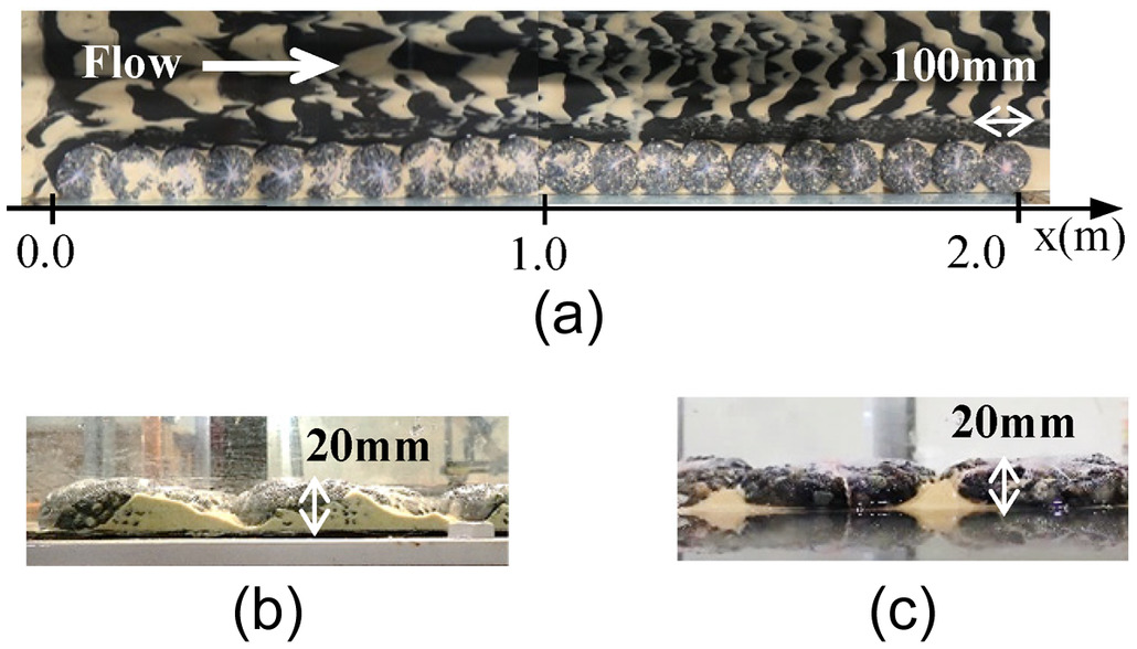
Fig. 7 shows the calculated sediment thickness at the time when the topographical changes stabilized (after approximately 30 min). The results captured the condition in which the sediment thickness was large in an approximately 1-m section on the upstream side and small on the downstream side, similar to the experiment. The calculated median sediment diameter ranged from 0.07 to 0.09 mm on the upstream side () and 0.06–0.07 mm on the downstream side (). The calculated and measured values of the sediment thickness are shown in Figs. 7(b and c). The measured value is the average of two runs, and the variation remained within 30%. On the wall side, the calculation result showed favorable agreement for the deposition peak value and deposition thickness decrease along the downstream direction regardless of the grid size. On the mainstream side, although the measured values varied, the tendency of the sediment thickness to decrease from upstream to downstream was reproduced. In the large-grid-size case, the sediment thickness was underestimated overall.
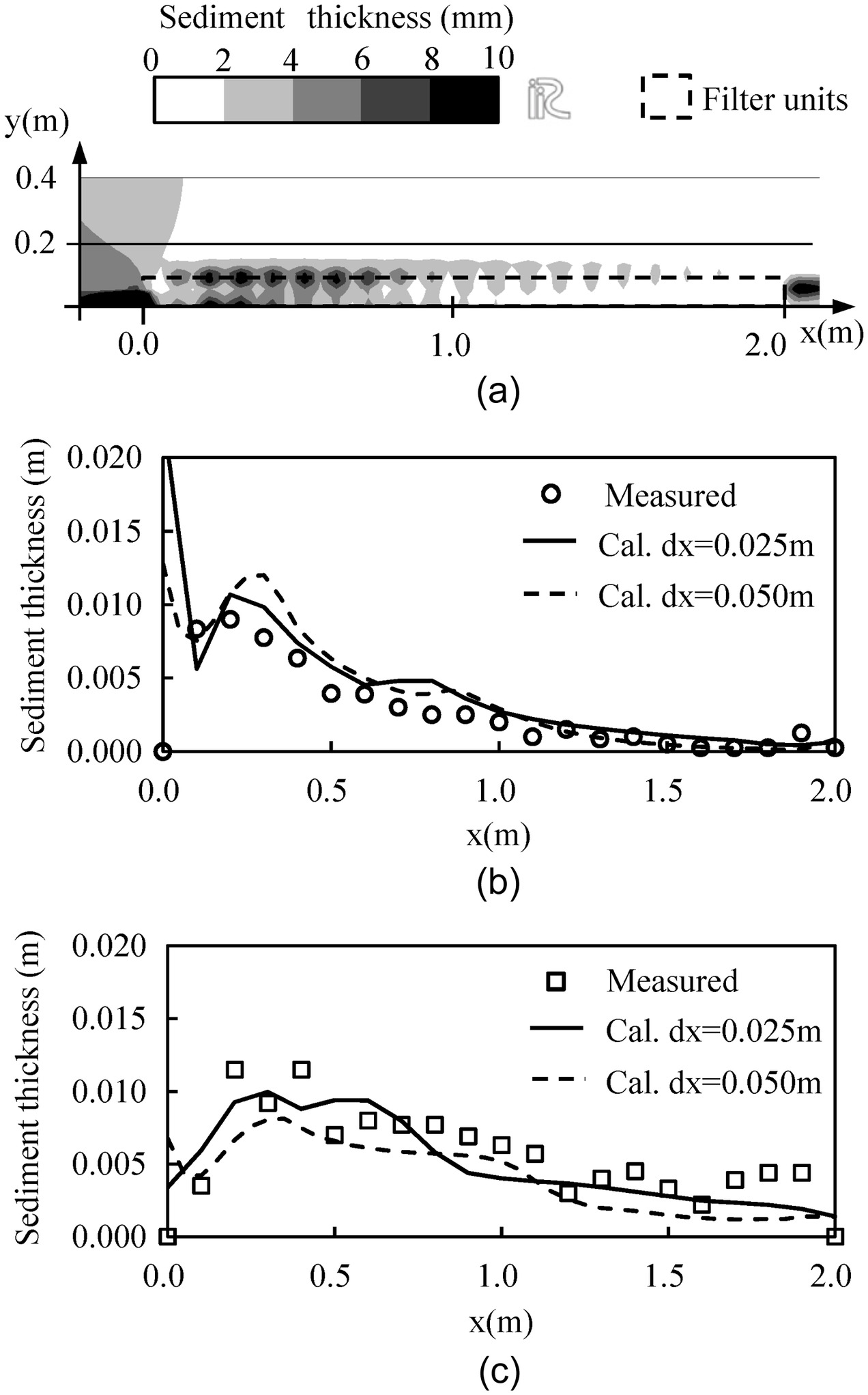
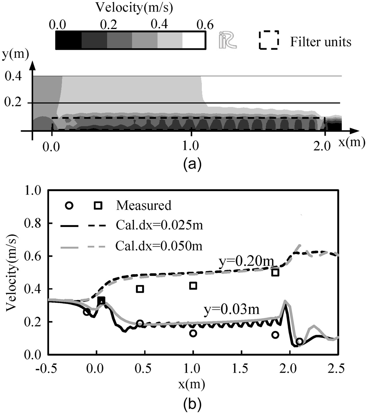
Fig. 8(a) shows the planar distribution of the calculated flow velocity values around the FUs in the case of . The flow velocity significantly decreased around the FUs and increased at the center of the channel. Behind the FUs (), the flow velocity was less than . Fig. 8(b) shows the flow velocities at the center of the channel () and the center of the FUs () along with the measured values. The measured value was the flow velocity at a 40% depth, which is considered to be the depth-average velocity (Ortiz et al. 2013). Although the vertical flow velocity distribution was measured in 0.01-m increments at several points for confirmation, the velocity remained almost uniform. The measured and calculated values were in good agreement. Although the calculated value was overestimated at the center of the channel, the error was less than 20%. The grid size did not affect the flow velocity calculation results except around the downstream end of the FU. The upstream end of the FU was approximately 0.01 m deeper than the downstream end due to the backwater effect of the FUs, and the depth from downstream of the FU to the end of the channel was almost uniform at 0.03 m. Therefore, the energy gradients were higher than the bed slope in the FU installation section. The water level along the transverse direction remained almost constant, and the measured water depth was mostly consistent with the calculated value.
Babame River Analysis
To examine FU placement for promoting sedimentation, numerical calculations were performed considering the actual riverbed grain size, river channel shape, and suspended sediment volume. Calculations were made in the following two cases:
Case 1: continuous FU placement; and
Case 2: placement at 1-m intervals for every 3 FUs.
Case 1 represents the current arrangement. In Case 2, it was considered that widening the interval could affect riverbed scouring, so the interval was set to 1 m, which is half the FU diameter. In each placement case, two types of floods were applied (Fig. 5).
Fig. 9 shows the riverbed fluctuations after the floods. In all cases, the riverbed was eroded on the left bank side, and sediment was deposited on the right bank side around No. 15.5 and No. 17.5. The grain size was coarser in areas where the riverbed was eroded. The deposition areas after the 2017 flood [Fig. 9(b)] corresponded to where sandbars appeared in aerial photographs after the actual 2017 flood (Hagiwara et al. 2022b).
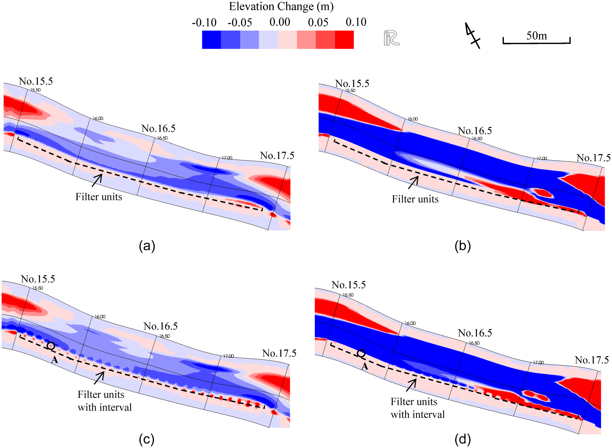
With continuous placement [Figs. 9(a and b)], there was remarkable sedimentation on the FUs in the section from No. 17 to No. 17.5, especially considering the 2017 flood, in which sediment was deposited beyond 0.1 m. The median grain size of sand deposited on the FUs was smaller than 10 mm. Sedimentation on the FUs was observed in this section [Fig. 3(a)]. In the section downstream from No. 16, the sediment thickness on the FUs was smaller than 1 mm regardless of the flood scale. In this section, the flow velocity on the left bank increased, and the riverbed around the FUs was scoured. It was considered that sediment was difficult to deposit in the water-colliding front in which the flow velocity increased.
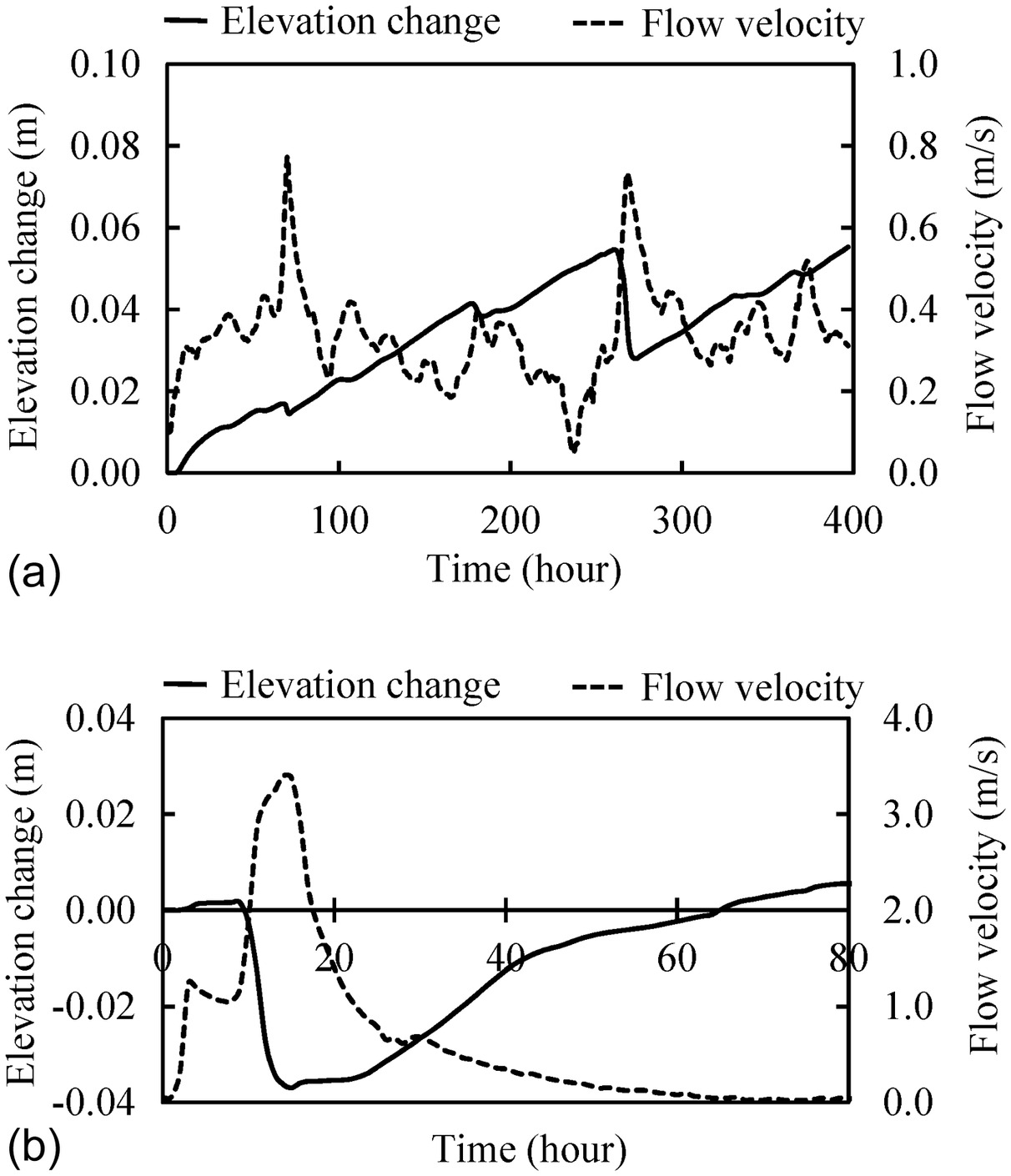
With interval placement [Figs. 9(c and d)], it was observed that the riverbed rose within the intervals between the FUs, and sediment was deposited even downstream from No. 16.0. In particular, there was remarkable sedimentation during the snowmelt flood, and the median grain size of the deposited sand was approximately 1 mm. Fig. 10 shows the time series of the flow velocity and elevation change at a representative point on the downstream side (Fig. 8, Point A). During the snowmelt flood, deposition gradually progressed and reached 0.06 m [Fig. 10(a)]. The flow velocity in the interval remained less than for a long period and reached less than half the surrounding flow velocity. Considering the 2017 flood, the riverbed within this interval was scoured due to the flow velocity increase, and sediment was deposited during the flood decay period [Fig. 10(b)]. Although the flow velocity within this interval was lower than that in the surrounding area, it increased to approximately at the flood peak, resulting in scouring within this interval. The amount of scouring and deposition was smaller than that of deposition during the snowmelt flood.
Discussion
Numerical Model Applicability
It was confirmed that the deposition thickness and flow around the FU could be reproduced with a two-dimensional model, except at the upstream end of the FU [Figs. 7(b and c), ]. Fukuoka et al. (1999) showed that the flow field around submerged continuously placed blocks can be calculated accurately with a two-dimensional model in cases in which the water depth is more than 1.3 times the block height. Because the water depth during this sedimentation experiment was 2 times the FU height, it was possible to express the flow field and sediment deposition around the submerged FUs. In addition, by setting the drag coefficient of the FU to only at the beginning, the calculation accuracy was improved relative to the case of for all FUs (Hagiwara et al. 2022b). However, complex flow occurred due to the sudden change in the riverbed height in front of the upstream end, which limits the applicability of the two-dimensional model. This study focused not only on the upstream end of the FU but also on the sediment deposition tendency around a series of FUs.
The RMS errors (RMSEs) of the sediment thickness on the bank and mainstream sides of the FUs (except at in Fig. 7) are presented in Table 1. The calculation accuracy was higher for deposition on the wall side than on the mainstream side, and the finer the calculation grid was, the higher the accuracy. In the case of the coarse grid (), the sediment thickness on the mainstream side was underestimated overall, which occurred because the unevenness of the FUs was not reflected well and the calculated flow velocity was higher, especially in the downstream FUs. In studies that calculated the sediment fluctuation around the groins using three-dimensional models, the RMSE ranged from 0.0018 to 0.0021 m (Choufu et al. 2019; Okhravi et al. 2023). Compared with these calculation results, the two-dimensional model used in this study sufficiently reproduced sediment deposition around the FUs. In particular, sand deposited on the mainstream side is washed away during high floods, so the sediment along the bankside is important. Sufficient calculation accuracy can be obtained even in the case of a grid size set to half the FU diameter.
| Case | RMSE (m) | |
|---|---|---|
| Wall side | Mainstream side | |
| 0.0013 | 0.0018 | |
| 0.0015 | 0.0021 | |
Continuous FU Placement
In the sedimentation experiment, remarkable coarse-sized sedimentation occurred on the upstream side of the continuously arranged FUs. On the downstream side, the sediment layer was thin and exhibited a fine grain size. Although sedimentation was observed around the upstream FUs within 5 min from the start of the experiment, most sand remained at the upstream end of the channel, suggesting that the sand deposited around the FU was suspended sediment transported along the current. Upstream of the FUs (), it was assumed that there was open channel flow with a laminar boundary layer because of the low Reynolds number (). The flow velocity decreased due to the backwater effect of the FUs. In addition, the flow was turbulent around the upstream FU (), resulting in a rapid decrease in the flow velocity and transition to a turbulent boundary layer (Ortiz et al. 2013). In the wake of the FUs (), it was assumed that the shear layer separated, forming a recirculation zone (Ortiz et al. 2013), and the flow velocity decreased locally. Decreasing the flow velocity led to reduced upward flux and transport of suspended sediment (Itakura and Kishi 1980; Gu et al. 2011), resulting in remarkable coarse-sized sedimentation around the upstream FUs. Although fine grains flowed around the downstream FUs, they were difficult to deposit because the flow velocity was not sufficiently low. Although actual rivers experience turbulent flow rather than the experimental laminar flow, the flow around the FUs was turbulent in the experiment, so the tendency of suspended sediment deposition would not differ greatly between the experiment and actual rivers.
Interval FU Placement
Placing the FUs at intervals resulted in sediment deposition within the intervals at low flow rates. It was considered that placing the FUs at intervals caused areas with a locally decreased flow velocity and inflow of suspended sediment from the main flow area, which promoted sediment deposition in the intervals. The flow within the interval is considered to be planar two-dimensional similar to the case of permeable groins (Gu et al. 2011). During extreme floods, the riverbed shearing force due to the current exceeds the critical shearing force of the riverbed material within the intervals, causing sand to flow out and the bed to be scoured (Ashida and Michiue 1972).
Fig. 11 shows the situation of a vacant spot spanning one FU width in the Babame River upstream of No. 17.0. Approximately 1 year had passed because the FUs were installed, and the river experienced one snowmelt flood and several summer floods. Sediment was deposited in the vacant spot, and after a few years, vegetation grew in the same way as on the FUs [Fig. 1(a)]. The vacant spot exerted no negative impact on the revetment. The field conditions also indicated that sediment would be deposited rapidly by placing the FUs at intervals. The riverbed within the intervals between the FUs was scoured during extreme floods, which may have a negative impact on the revetment in the long term. However, by promoting sediment deposition within the intervals over a short period, vegetation can grow and improve the erosion resistance of the intervals (Ikeda and Izumi 1990) before an extreme flood occurs.
Impact of FU Placement
To examine effective placement for promoting sediment deposition, various FU placement calculations were performed for Section no. 15.5–16.0, in which scouring within the intervals was intense. The diameter of a single FU is denoted , the sediment thickness (or scour depth) within the FU interval is denoted , the distance between adjacent FUs is denoted , and the interval length is denoted [Fig. 12(a)]. For placement with varying and values, two types of flow rates were applied: an average snowmelt flow rate of , and a maximum flow rate of . The calculation was performed until the riverbed within the intervals did not change under a constant flow rate. Fig. 12(b) shows the result with , and the interval length was adjusted from to 2; denotes the number of FU rows. Fig. 12(c) shows the result with , and the FU row was adjusted from to 5. At a flow rate of , the sediment thickness stabilized within 300 h. At a flow rate of , the scoured depth stabilized within 5 h. The sediment thickness and water depth normalized by the FU height are shown. For , scouring increased with increasing interval. In the case of , the scouring depth was approximately 0.1 times the FU height, which was less than half the sediment thickness due to the snowmelt flood. The FU interval should be as short as possible in order to minimize scouring and the fluid force acting on the FU (Fukuoka et al. 1999).
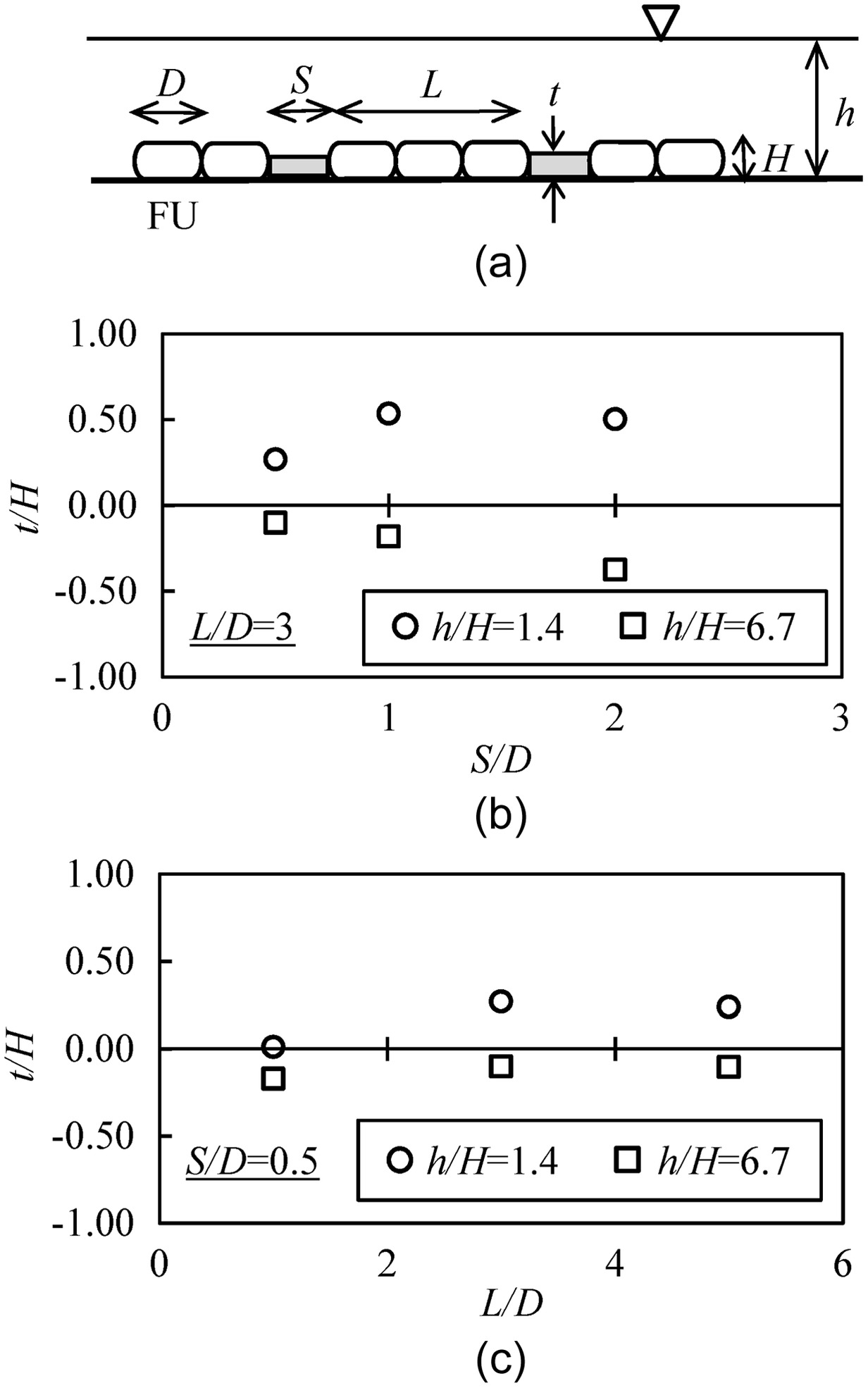
For , in the case of , the sediment thickness reached 0.25 times the FU height at a low flow rate. In this case, it could be expected that sediment gradually would be deposited in the intervals and that vegetation would grow. In the case of , sediment would not accumulate in the intervals, and the riverbed would continue to decline. Effective FU placement to promote sedimentation entailed employing an interval of half the FU width for every three or more FUs. Although sedimentation was not promoted on the FU, it can be considered that vegetation growth would increase the water flow resistance and expand the surrounding sediment deposition range (Kim et al. 2018).
The present findings can be applied to small and medium-sized rivers with riverbed gradients of approximately 1/500. Although the analysis was performed with 2-t-type FUs as the target, larger FUs could be used in rivers in which the design velocity exceeds the applicable range of 2-t-type FUs. Even in such a case, the amount of suspended sediment will increase with increasing flood scale, so the relationship between FU placement and sedimentation is considered to hold. However, the maximum size of the FUs is 4 t, and this FU type cannot be applied in rivers in which the design flow velocity exceeds , which is the stable critical flow velocity calculated from the balance between the fluid force and FU weight. When large FUs are used for the design flow velocity (for example, 4-t-type FUs used where 2-t-type FUs are sufficient), deposition could increase and scouring could decrease in the intervals because the resistance of the FU increases. However, the use of large FUs leads to high construction costs. Additionally, rivers with a gentle slope and deep water could yield different results, because the installed FUs would always be submerged. It is necessary to investigate sedimentation around FUs considering various conditions.
Conclusions
This study investigated a method by which suspended sediment is deposited across a large area around FUs by examining the surrounding topographical changes and various placements using hydraulic experiments and numerical calculations. The main conclusions of this study are as follows:
1.
The sedimentation hydraulic experiment involving continuous FU model placement showed that coarse sand was deposited in the area in which the flow velocity decreased around several FUs on the upstream side. Although fine sand flowed into the FU on the downstream side, very little was deposited because the flow velocity was not sufficiently low.
2.
Arranging FUs at intervals resulted in sediment deposition within the intervals even on the downstream side. Sedimentation within the intervals was due primarily to floods that persisted for a long period, such as snowmelt floods. During the extreme flood in which the flow rate rapidly increased, the riverbed within the intervals was scoured at the peak flow rate, but sediment was redeposited during the flood decay period.
3.
Increasing the FU interval caused an increase in sediment deposition during snowmelt floods and an increase in the scouring depth during extreme floods. Furthermore, decreasing the consecutive FU length (number of rows) reduced sediment deposition in the intervals. Effective FU placement for promoting sedimentation involved employing an interval of half the FU width for every three or more FUs.
Vegetation can grow on the deposited sediment within the intervals, further promoting sedimentation around the FUs. The findings can be applied to small and medium-sized rivers with riverbed gradients of approximately 1/500. Further investigation is needed for rivers considering various conditions.
Data Availability Statement
All of the data, models, or code that support the findings of this study are available from the corresponding author upon reasonable request.
Acknowledgments
The Akita Regional Development Bureau of Akita Prefecture provided the Babame River topographical and water level data for this study. The riverbed grain size and riverbed crossing data were provided by the Department of Civil and Environmental Engineering, Akita University. The authors express their gratitude. This research was partially supported by the Ministry of Education, Science, Sports and Culture, Grant-in-Aid for Scientific Research (A: 20H00256, So Kazama; B: 23H01508, Yoshiyuki Yokoo), and the Environment Research and Technology Development Fund (JPMEERF20S11813) of the Environment Restoration and Conservation Agency of Japan. The authors thank Editage (www.editage.com) for the language editing.
References
Alauddin, M., and T. Tsujimoto. 2012. “Optimum configuration of groynes for stabilization of alluvial rivers with fine sediments.” Int. J. Sediment Res. 27 (2): 158–167. https://doi.org/10.1016/S1001-6279(12)60024-9.
Ali, S., and W. S. J. Uijttewaal. 2013. “Flow resistance of vegetated weirlike obstacles during high water stages.” J. Hydraul. Eng. 139 (3): 325–330. https://doi.org/10.1061/(ASCE)HY.1943-7900.0000671.
Ashida, K., S. Egashira, B. Liu, and M. Umemoto. 1990. “Sorting and bed topography in meander channels.” Annu. Disaster Prev. Res. Inst. Kyoto Univ. 33 (B-2): 261–279.
Ashida, K., and M. Michiue. 1972. “Study on hydraulic resistance and bedload transport rate in alluvial stream.” Proc. Jpn. Soc. Civ. Eng. 1972 (206): 59–69. https://doi.org/10.2208/jscej1969.1972.206_59.
Choufu, L., S. Abbasi, H. Pourshahbaz, P. Taghvaei, and S. Tfwala. 2019. “Investigation of flow, erosion, and sedimentation pattern around varied groynes under different hydraulic and geometric conditions: A numerical study.” Water 11 (2): 235. https://doi.org/10.3390/w11020235.
Ezzeldin, R. M. 2019. “Numerical and experimental investigation for the effect of permeability of spur dikes on local scour.” J. Hydroinf. 21 (2): 335–342. https://doi.org/10.2166/hydro.2019.114.
Fukuoka, S., T. Kabasawa, J. Saito, Y. Fuse, A. Watanabe, and M. Ohashi. 1998. “Field tests on groin utilizing natural willows.” Proc. Hydraul. Eng. 42 (Feb): 445–450. https://doi.org/10.2208/prohe.42.445.
Fukuoka, S., T. Miyagawa, and M. Tobiishi. 1997. “Measurements of flow and bed geometry around a cylindrical pier and calculation of its fluid forces.” Proc. Hydraul. Eng. 41 (Feb): 729–734. https://doi.org/10.2208/prohe.41.729.
Fukuoka, S., M. Mizuguchi, T. Uchida, and H. Yokoyama. 1999. “Study of shallow water flow with submersible and non-submersible large-roughness.” Proc. Hydraul. Eng. 43 (Feb): 293–298. https://doi.org/10.2208/prohe.43.293.
Giglou, A. N., J. A. Mccorquodale, and L. Solari. 2018. “Numerical study on the effect of the spur dikes on sedimentation pattern.” Ain Shams Eng. J. 9 (4): 2057–2066. https://doi.org/10.1016/j.asej.2017.02.007.
Gu, Z.-P., R. Akahori, and S. Ikeda. 2011. “Study on the transport of suspended sediment in an open channel flow with permeable spur dikes.” Int. J. Sediment Res. 26 (1): 96–111. https://doi.org/10.1016/S1001-6279(11)60079-6.
Hagiwara, T. 2023. “The impact of the filter units on sediment deposition and vegetation.” Doctoral thesis, Dept. of Civil Engineering, Tohoku Univ.
Hagiwara, T., S. Aita, and S. Kazama. 2020. “A suggestion of effective block arrangements which promote deposition of suspended sediment around foot protection block.” J. Jpn. Soc. Civ. Eng. Ser. B1 76 (2): 1189–1194. https://doi.org/10.2208/jscejhe.76.2_I_1189.
Hagiwara, T., S. Aita, and S. Kazama. 2022a. “Impact of vegetation grown around the filter units on the river revetment.” J. Jpn. Soc. Civ. Eng. Ser. G 78 (5): 135–142. https://doi.org/10.2208/jscejer.78.5_I_135.
Hagiwara, T., S. Aita, K. Watanabe, and S. Kazama. 2022b. “A numerical analysis about suspended sediment deposition around filter unit.” In Proc., 39th IAHR World Congress, 2590–2598. Granada, Spain: International Association for Hydro-Environment Engineering and Research.
Ikeda, S., and N. Izumi. 1990. “Width and depth of self-formed straight gravel rivers with bank vegetation.” Water Resour. Res. 26 (10): 2353–2364. https://doi.org/10.1029/WR026i010p02353.
Ikeda, S., N. Izumi, and R. Ito. 1991. “Effects of pile dikes on flow retardation and sediment transport.” J. Hydraul. Eng. 117 (11): 1459–1478. https://doi.org/10.1061/(ASCE)0733-9429(1991)117:11(1459).
Itakura, T., and T. Kishi. 1980. “Open channel flow with suspended sediments.” J. Hydraul. Div. 106 (8): 1325–1343. https://doi.org/10.1061/JYCEAJ.0005483.
Iwagaki, Y. 1956. “Hydrodynamical study on critical tractive force.” Trans. Jpn. Soc. Civ. Eng. 1956 (41): 1–21. https://doi.org/10.2208/jscej1949.1956.41_1.
Iwasaki, T., M. Nabi, Y. Shimizu, and I. Kimura. 2015. “Computational modeling of 137Cs contaminant transfer associated with sediment transport in Abukuma River.” J. Environ. Radioact. 139 (Jan): 416–426. https://doi.org/10.1016/j.jenvrad.2014.05.012.
Johannesson, H., and G. Parker. 1989. “Secondary flow in mildly sinuous channel.” J. Hydraul. Eng. 115 (3): 289–308. https://doi.org/10.1061/(ASCE)0733-9429(1989)115:3(289).
Kaseguma, K., S. Maeno, K. Yoshida, D. Takata, and A. Yamamura. 2013. “Evaluation of hydrodynamic force acting on revetment and bed protection blocks in supercritical flow.” J. Jpn. Soc. Civ. Eng. Ser. B1 69 (4): 691–696. https://doi.org/10.2208/jscejhe.69.I_691.
Kawamura, C., Y. Shimizu, M. Fujita, and Y. Ichikawa. 1997. “Field measurements and analysis of sediment in a mountain river.” Proc. Hydraul. Eng. 41 (Feb): 771–776. https://doi.org/10.2208/prohe.41.771.
Kim, H. S., I. Kimura, and M. Park. 2018. “Numerical simulation of flow and suspended sediment deposition within and around a circular patch of vegetation on a rigid bed.” Water Resour. Res. 54 (10): 7231–7251. https://doi.org/10.1029/2017WR021087.
Kovacs, A., and G. Parker. 1994. “A new vectorial bedload formulation and its application to the time evolution of straight river channels.” J. Fluid Mech. 267 (May): 153–183. https://doi.org/10.1017/S002211209400114X.
Kyuka, T., H. Takebayashi, and M. Fujita. 2016. “Effect of angle of spur dikes on flow, bed load and bed variation characteristics.” J. Jpn. Soc. Civ. Eng. Ser. B1 72 (4): 805–810. https://doi.org/10.2208/jscejhe.72.I_805.
Mohamed, H. I. 2010. “Flow over gabion weirs.” J. Irrig. Drain. Eng. 136 (8): 573–577. https://doi.org/10.1061/(ASCE)IR.1943-4774.0000215.
Okhravi, S., S. Gohari, M. Alemi, and R. Maia. 2023. “Numerical modeling of local scour of non-uniform graded sediment for two arrangements of pile groups.” Int. J. Sediment Res. 38 (4): 597–614. https://doi.org/10.1016/j.ijsrc.2023.04.002.
Ortiz, A. C., A. Ashton, and H. Nepf. 2013. “Mean and turbulent velocity fields near rigid and flexible plants and the implications for deposition.” J. Geophys. Res.: Earth Surf. 118 (4): 2585–2599. https://doi.org/10.1002/2013JF002858.
Shimizu, Y., H. Takebayashi, T. Inoue, M. Hamaki, T. Iwasaki, and M. Nabi. 2014. “iRICNays-2DH solver manual.” Accessed January 25, 2022. https://i-ric.org/en/download/nays2dh-menual-v3/.
Steiros, K., K. Kokmanian, N. Bempedelis, and M. Hultmark. 2020. “The effect of porosity on the drag of cylinders.” J. Fluid Mech. 901 (Oct): R2. https://doi.org/10.1017/jfm.2020.606.
Tanaka, N., J. Yagisawa, and S. Otsuka. 2014. “Method for evaluating the forestation in a river considering the characteristics of flood decline and geomorphology of gravel bars on the deposition of fine sand.” J. Jpn. Soc. Civ. Eng. Ser. B1 70 (3): 60–70. https://doi.org/10.2208/jscejhe.70.60.
Tingsanchali, T., and S. Maheswaran. 1990. “2-D depth-averaged flow computation near groyne.” J. Hydraul. Eng. 116 (1): 71–86. https://doi.org/10.1061/(ASCE)0733-9429(1990)116:1(71).
Yamamoto, K., K. Hayasi, M. Sekine, K. Fujita, M. Tamura, K. Nisimura, and K. Hamaguchi. 2000. “Measuring method of drag coefficient, lift coefficient and equivalent roughness of revetment block.” Proc. Hydraul. Eng. 44 (Feb): 1053–1058. https://doi.org/10.2208/prohe.44.1053.
Yoon, T., and Y. Kim. 2005. “Effects of a vegetation zone on flow and scour depth around a downstream bridge pier.” In Proc., 31st IAHR World Congress, 1561–1569. Seoul, South Korea: International Association for Hydro-Environment Engineering and Research.
Information & Authors
Information
Published In

Journal of Hydraulic Engineering
Volume 150 • Issue 6 • November 2024
Copyright
This work is made available under the terms of the Creative Commons Attribution 4.0 International license, https://creativecommons.org/licenses/by/4.0/.
History
Received: Sep 1, 2023
Accepted: May 28, 2024
Published online: Aug 6, 2024
Published in print: Nov 1, 2024
Discussion open until: Jan 6, 2025
ASCE Technical Topics:
- Bodies of water (by type)
- Coasts, oceans, ports, and waterways engineering
- Engineering fundamentals
- Environmental engineering
- Filters
- Filtration
- Hydraulic engineering
- Hydraulic structures
- Model accuracy
- Models (by type)
- River engineering
- Rivers and streams
- Sediment
- Structural engineering
- Structures (by type)
- Suspended sediment
- Suspended structures
- Two-dimensional models
- Water and water resources
- Water management
- Water treatment
- Waterways
Authors
Metrics & Citations
Metrics
Citations
Download citation
If you have the appropriate software installed, you can download article citation data to the citation manager of your choice. Simply select your manager software from the list below and click Download.