Implementation of Standardized Uncertainty Analysis for Streamflow Measurements Acquired with Acoustic Doppler Velocimeters
Publication: Journal of Hydraulic Engineering
Volume 150, Issue 6
Abstract
This paper discusses a full-fledged uncertainty analysis implementation using the Guide to the Expression of Uncertainty in Measurement (GUM) as framework. Currently, there are few examples of rigorous GUM implementations in hydrometry. This work fills this gap by demonstrating the use of the GUM framework to estimate the uncertainty of open-channel discharge measurements conducted with the velocity-area method using acoustic doppler velocimeters. The paper first presents the GUM protocol and the steps leading to discharge measurement followed by evaluations of Type A uncertainty from customized experiments, Type B uncertainty informed by prior experiments and engineering judgment, and the total discharge uncertainty. Finally, the uncertainty analysis (UA) implications and practical usage for data management and improvement of measurement processes are discussed. While the detail of the analysis can be further increased, the main role of this paper is to illustrate a step-by-step implementation of GUM procedures applied to natural-scale measurements using a GUM-compliant software.
Introduction
Streamflow data are core inputs for decision making for water management, energy development, infrastructure design, emergency forecasting, ensuring water quality, ecosystem viability, and recreational uses. Streamflow data are also used as benchmarks for scientific studies on water cycle, ecological patterns, climate change, and the continuous growth of water consumption for societal and environmental demands. These data are routinely collected by multiple specialized agencies with measurement protocols developed and successively refined through century-long incremental developments (USGS 1994). The methods for the measurement of streamflow are typically based on empirical or semi-empirical relationships (i.e., rating curves) established with statistical analyses applied to long records of directly measured stream discharges (Rantz 1982; Levesque and Oberg 2012). Direct measurements of flow discharges can be obtained with a wide variety of instruments and methods (Rennie et al. 2017). The most popular contemporary instruments for streamflow quantification are based on acoustic technologies (Muste et al. 2007).
While the methods for direct measurements of streamflow have made swift progress due to advancement in science and technologies, the methods for assessing the quality of the measured data are lagging. This is unfortunate because there is a need for reporting streamflow measurements along with their measurement uncertainty for any of the data final use (i.e., scientific, applied, or commercial). Providing streamflow measurement uncertainty should become a standard professional practice, as the data are used not only in basic and applied research but also for complying with laws, regulations, and quality control constraints (McMillan et al. 2012; Bertrand-Krajewski et al. 2021). The quality of the measurements is typically quantified with uncertainty analyses (UA). Currently, the hydrometric community has not converged to one widely recognized UA framework. Instead, uncertainty estimations are obtained with multiple standards applied to specific variables and measurement methods or through instrument intercomparison (e.g., Reader-Harris 2007; Le Coz et al. 2016, respectively). This situation concerns the hydrometric community, which seeks sound UA procedures that are uniformly applicable across instruments and variables and that meet stringent quality requirements.
The fundamental features of a sound uncertainty assessment procedure [JCGM 100 (JCGM 2008a)] as follows: universality (applicable to diverse measurements), internal consistency (directly derivable from the components that contribute to the total uncertainty), and transferability (usable for both primary and derived quantities). Fortunately, in the last three decades significant progress has been made toward the adoption of uncertainty assessment frameworks that fulfill the abovementioned requirements. A leading role in this progress has been played by the publication of the Guide to Expression of Uncertainty in Measurement (GUM 1995), which is broadly considered as an authoritative uncertainty methodology. The GUM framework offers general rules for evaluating and expressing uncertainty in measurement rather than providing detailed instructions tailored to specific fields of study. Following its initial publication, the GUM has been lightly revised during its adoption by various international metrological organizations. Since 2000, the Joint Committee for Guides in Metrology (JCGM) has been responsible for GUM updates and distribution; hence, the GUM framework is widely referred to as JCGM 100 (JCGM 2008a). Several engineering communities have “harmonized” their standards by adopting GUM as a guideline, as illustrated by the World Meteorological Organization recommendation to National Meteorological and Hydrological Services (Muste 2017a), the International Organization for Standardization’s (ISO) new hydrologic uncertainty guidance (ISO 2020), and the recently published guidance for urban hydrometry (Bertrand-Krajewski et al. 2021).
The goal of this paper is to demonstrate the versatility and feasibility of applying the GUM framework to hydrometric measurements. Currently, there are few examples and practical guidelines for rigorous GUM implementation in hydrometry. This paper fills this gap by demonstrating the use of the GUM framework to estimate the uncertainty of open-channel streamflow measurements conducted with the velocity-area method using acoustic doppler velocimeters (ADV). The paper presents first the GUM protocol and the procedure to determine discharge with an ADV, followed by evaluations of elemental and total uncertainties for discharge measurement acquired through a dedicated case study. Finally, UA implications and practical usage for data management and improvement of measurement processes are discussed.
UA Considerations
The evaluation of uncertainty is neither a routine task nor a purely theoretical one; it depends on detailed knowledge of the nature of the measurand, instrument, the measurement process, and the measurement environment in which a specific measurement is executed. The GUM framework is straightforward and precise regarding the statistical and mathematical procedures to be followed in UA, while its practical implementation is based on assumptions and evaluations that are not prescribed in full details. In other words, the laws of uncertainty assessment and propagation are generic and uniformly applied for elemental and compounded uncertainties, while the practical means to obtain these estimates are decided by the domain specialist. Consequently, the quality and utility of the uncertainty quoted for the result of a measurement depend on the professional skills and integrity of those who contribute to the estimation of its value [JCGM 100 (JCGM 2008a); Beven et al. 2017].
GUM Essentials
The GUM framework is based on uniform use of mathematical statistics principles for propagating elemental sources of errors to final results. With the assumption that the reader is broadly familiar with UA, we provide herein only essential elements of GUM implementation (see Fig. 1). More details about GUM framework implementation can be found in Muste et al. (2012) and Muste (2017b). Details on the estimation of individual sources of uncertainties associated with acoustic instruments such as ADVs and acoustic doppler current profilers (ADCPs) can be found in Muste et al. (2004), Gonzalez-Castro and Muste (2007), Muste et al. (2010), and Lee et al. (2014). The UA calculations presented in this paper are facilitated by GUM software package QMSys Enterprise via the QMSys Calculator, a customized version of the software for hydrometric measurements (QualiSyst 2019).
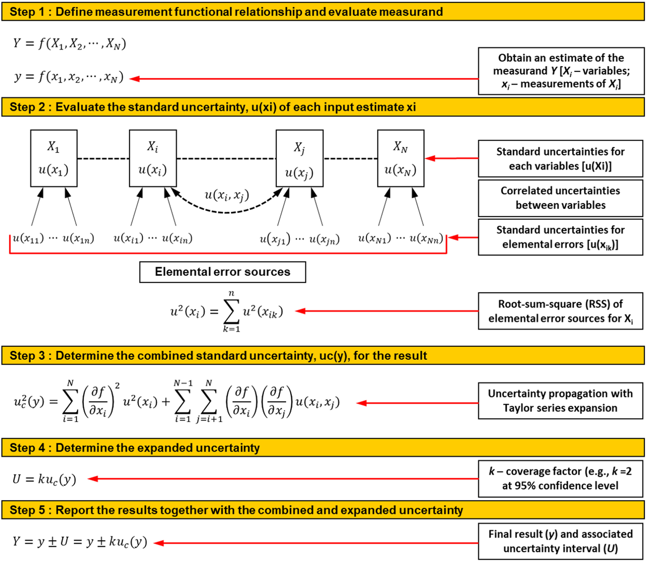
The UA robustness depends on the efforts and details placed in Step 1 (definition of the measurement process) and Step 2 (identification of all uncertainties associated with the functional relationship of the measurement process and making decisions on what type of estimation methods are used for the evaluation of these uncertainties, i.e., Type A or B). Type A uncertainties are evaluated by statistical means applied to data collected during the current measurements; Type B uncertainties are determined by other means (i.e., previous experiments or technical judgement). Computer scripts for Type A and B evaluations are available in sections “Type A Method for Uncertainty Assessment of Repeated Measurements”–“Type B Method for Uncertainty Assessment by the Law of Propagation of Uncertainties” of Bertrand-Krajewski et al. (2021). Steps 1 and 2 are complex, tedious, and costly, as they entail identification and assessment of all possible uncertainties affecting the data acquisition chain, from the probe sensing the flow to the data display (including signal conversion, conditioning, and internal processing), and uncertainties induced by methods, operations, and environmental conditions. Steps 3, 4, and 5 are merely algebraic calculations that can be automated using simple processing scripts.
Strictly speaking, each new hydrometric measurement is characterized by its own uncertainty. Even if the instrument protocols and methods are the same, measurements are taken at specific sites and times characterized by a unique measurement environment in terms local factors and influences. From this perspective, robust (fully fledged) UAs need rigorous organization and execution, with considerations of all sources of errors affecting the measurement functional relationship. If the measurements for all the input quantities in the functional relationship are repeated (ideally more than 10 times), the total uncertainty can be evaluated by Type A method. However, because this is rarely possible in practice due to limited time and resources, the uncertainty of a measurement result can be executed at various levels of rigor that need to be documented. When limited or no resources are available to conduct Type A evaluations, the JCGM (100:2008) accepts uncertainties estimated by the Type B evaluation method. Because the mathematical model of the measurement process may be incomplete, all relevant quantities should be varied to the fullest practical extent so that the evaluation of the uncertainties replicates as much as possible the potential range of the observed data. This is easily done with numerical simulations via the Monte Carlo method (MCM) tempered by engineering judgement (JCGM 101:2008).
Measurement Method: Velocity-Area
The measurement of streamflow benefits from extensive past developments and the continuous adoption of new measurement technologies (Rennie et al. 2017). Historically, the most popular method to directly measuring streamflow in natural channels of all sizes is based on point-velocity measurements used in conjunction with the velocity-area (VA) discharge estimation method. There are multiple published resources detailing VA alternatives and their practical implementation for a variety of instruments (e.g., Rantz 1982; Herschy 2009); therefore, we will not repeat that information here. Provided below are the terminology and notations along with information about the measurement method, instrumentation, and protocol that are relevant for the UA presented in the next sections. It should be noted upfront that the VA method applied in this case study is customized to reflect the changes brought about by the recently revised hydrometry uncertainty guidance (ISO 2020).
The measurement of discharge for a stream ensues from integration over the cross section of the mean velocity for a point velocity, , multiplied by the elemental area, , for which this mean velocity is representative
(1)
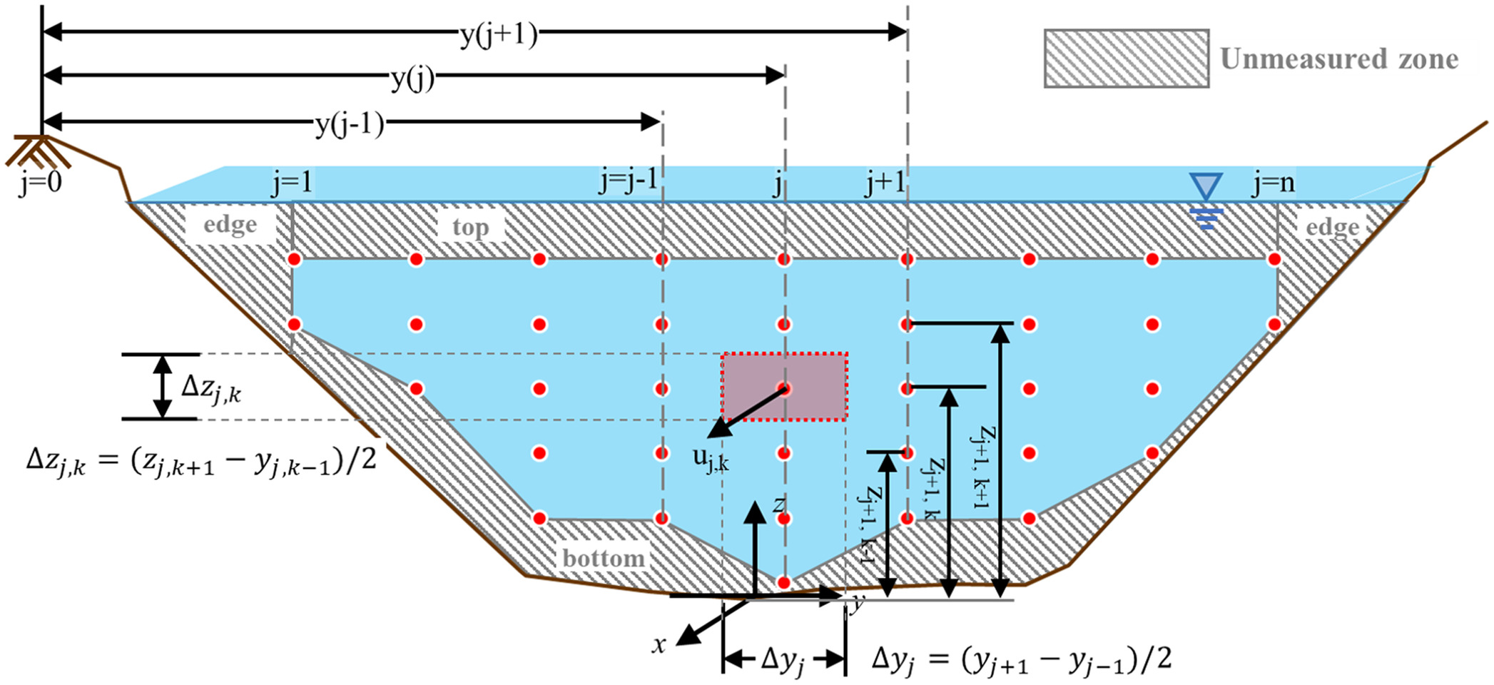
The mean cross-sectional velocity is obtained by sampling multiple-point velocities over the cross-section extent (see the measurement grid defined by indices , in Fig. 2). Specifically, mean point velocities, (, ), and the location of their measurement—i.e., the position of the vertical from the bank, , and the vertical location ()—are measured across the section. Elemental discharges are determined by the mean velocity, , associated with and elemental cross section, . Multiple verticals are collected over the cross section with each vertical containing multiple point velocity measurements. As correctly pointed out in HUG (ISO 2020), instruments cannot measure at (or near) the bed and free surface, leaving portions of the cross section unmeasured (see Fig. 2). Accounting for this realization and using notations in Fig. 2, the total stream discharge, , is obtained as the sum of all measured elemental discharges, , complemented by the unmeasured area discharges, (ISO 2020), as follows:where and = factors accounting for the discrete summation of the elemental discharges in the and directions, respectively. Obviously, the more points sampled within the measured area and the closer the measurements near free-surface and boundaries, the better the estimate of the cross-sectional (bulk flow) velocity. The impact of the and factors prescribed by HUG (ISO 2020) diminishes if the density of points is increased.
(2)
Eq. (2) is a generic expression for the VA midsection approach recommended in HUG (ISO 2020). The equation can be applied for a common measurement situation when just one point is sampled in the vertical. Eq. (2) serves well for defining the functional relationship of the measurand (Step 1 in Fig. 1) for a wide range of instruments and methods. This new formulation for the functional relationship provided in HUG (ISO 2020) departs from previous standards on VA method (e.g., ISO 748) by explicitly including the unmeasured areas of the cross section. Eq. (2) can be customized to accommodate various VA measurement protocols [e.g., velocity measurements from fixed verticals or moving boat, midsection or mean-section VA, index-velocity, or entropy-based bulk velocity estimation, as described by Chiu and Chen (1998)] and instruments (e.g., mechanical and electromagnetic meters, ADV, ADCP, and large-scale particle image velocimetry). Such customization is illustrated in the case study presented below.
Measurement Instrument: ADV
Acoustic instruments have proven to be reliable and efficient alternatives for measurement of velocities in open channel flows. Their use continues to expand due to the lack of moving parts, nonintrusive nature, and ease of deployment and operation compared with previous generations of velocimeters. Consequently, ADVs have experienced considerable growth in the last three decades, becoming leading tools for field studies in several countries. A representative probe from this category is the ADV produced by SonTek/YSI (San Diego) that will be used herein to illustrate UA implementation. Various aspects of ADV configuration, operation, and performance are covered by instrument producers (e.g., SonTek 1997) and other published references (e.g., Kraus et al. 1994; Goring and Nikora 1998; Voulgaris and Trowbridge 1998; McLelland and Nicholas 2000; Dombroski and Crimaldi 2007). The schematic of the SonTek ADV configuration is shown in Fig. 3(a). The specifications for the 16-MHz MicroADV used in this study are shown in Fig. 3(b) (Sontek 2017).
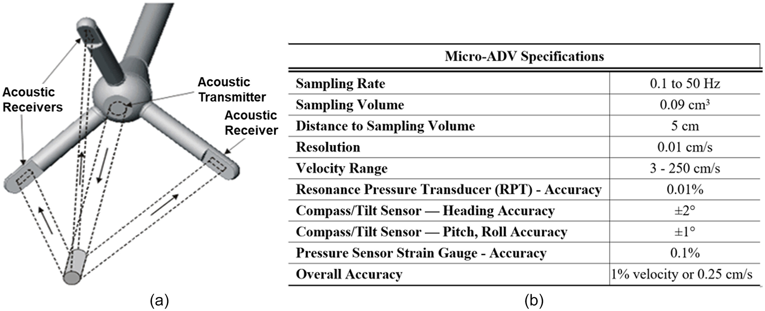
Assuming familiarity of the readers with ADV-related resources, we will only focus on instrument aspects related to UA. ADVs are instruments that measure velocities of small particles suspended in the flow, assuming that these particles travel at the same velocity as the water (Rehmel 2007). The cylinder-like ADV measurement volume is located a short distance from the acoustic sensor [see Fig. 3(a)]. When the ADV is fully submersed, the sound pulses emitted from transmitters are reflected in all directions by particles contained in the instrument measurement volume. A portion of the reflected energy is directed toward the receivers and captured as a voltage proportional to the instantaneous backscattered pressure (Lemmin 2017). If the particles are moving with respect to the probe, the backscattered sound will have a different acoustic frequency. The change in frequency “sensed” by each receiver is subsequently used to estimate the flow velocity through the following functional expression:where = flow velocity along the bistatic axis; = speed of sound in water; and = difference in the acoustic frequency between the emitted () and return () pulses due to doppler shift (). The bistatic axis is the line dividing the angle between the transmitter and receiver whose vertex is at the center of the sampling volume (Kraus et al. 1994). One transmitter and three receivers resolve three velocity components. The bistatic velocities acquired by the three acoustic sensors can be transformed into a cartesian coordinate system by the instrument software using the following relationship (Kraus et al. 1994):where , , and = velocity components expressed in instrument coordinate system; , , and = frequency differences sensed by the three receivers; and = geometrical transformation matrix that relates to the arrangement of the three receivers with respect to the central emitter. These equations are applied to each acoustic pulse, leading after internal or external processing to time-averaged velocity components, fluctuating components, and higher-order correlations.
(3)
(4)
UA Implementation
Measurement Protocol
The measurement protocol is critical for UA implementation because it dictates the structure of the measurement definition and the association of the elemental uncertainty sources to the measurement process components. As each experiment is unique from multiple perspectives, we illustrate in the next sections the UA-GUM implementation for the measurement protocol employed in a case study. This protocol follows the HUG (ISO 2020) formulation recommended for the midsection VA method in conjunction with point-velocity measurements [see Eq. (2)]. The presented protocol differs slightly from the typical midsection VA measurement method described by ISO 748 (ISO 2007a) that is widely popular in national hydrologic services for both traditional and emerging instruments (WMO 2017). The difference is minor, entailing the estimation of the discharges in the unmeasured area around the boundaries, i.e., in Eq. (2) that are not explicitly refer to in ISO 748 (ISO 2007a). Description of the midsection method including explicitly edge discharges is also used in Herschy (2009) and in the section by section discharge measurements with ADCPs (Mueller et al. 2007).
In the present case study, velocities and water depths are sampled in verticals distributed throughout the section, as shown in Fig. 4. For each velocity measurement point, the following variables are recorded: distance of vertical from the start bank, , water depth at the th vertical location, , and the mean point-velocity values, , measured at a point, . Illustration of the point-velocity measurements taken in the panel centered on vertical are visualized in Fig. 4.
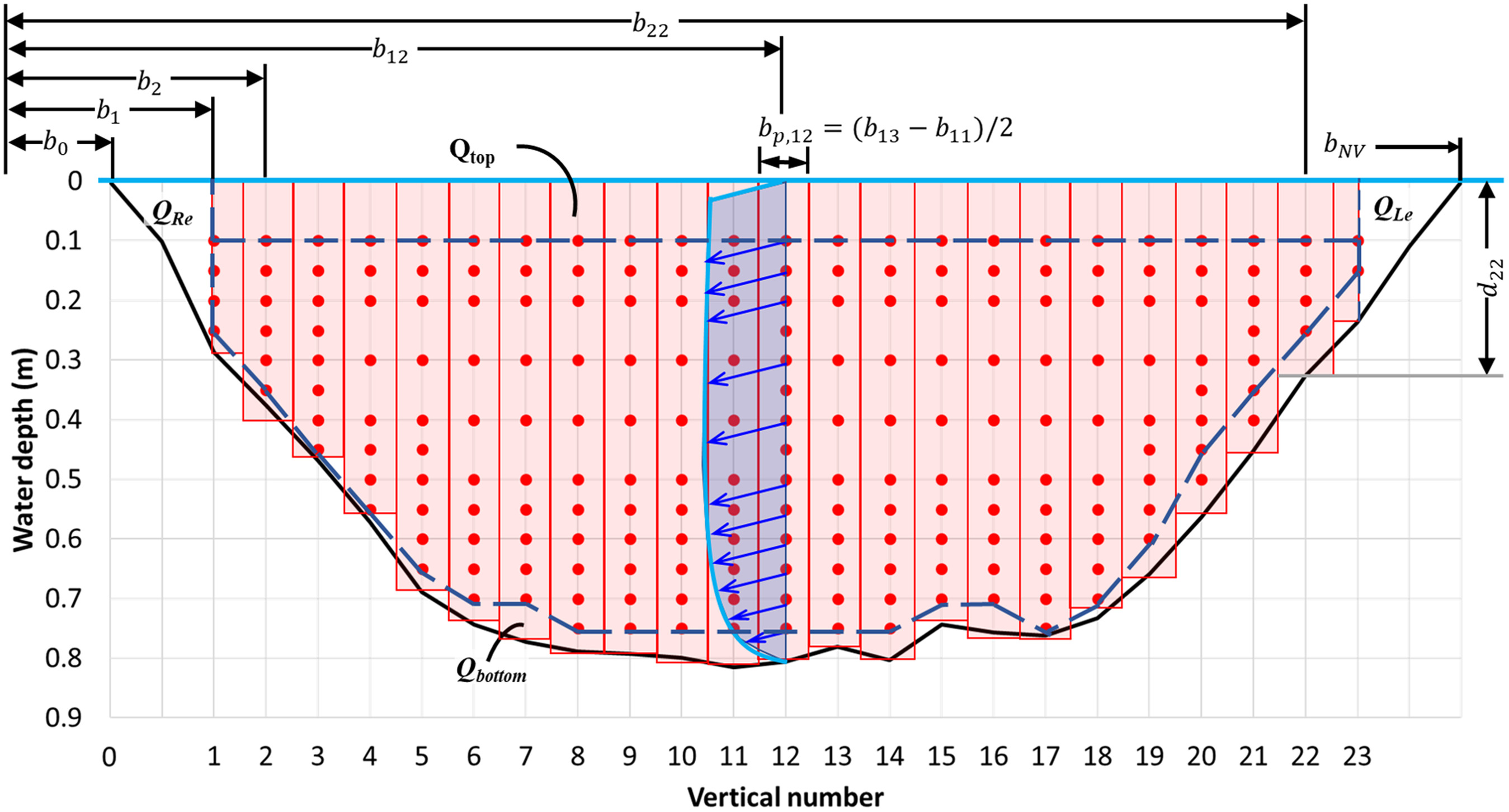
To reconcile differences between HUG generic equation [see Eq. (2)] and the typical VA implementation (Turnipseed and Sauer 2010; WSC 2015), we associate the velocities in the unmeasured areas near the top and bottom of the verticals to the depth-averaged velocity (see ISO 748, 2007, Section 8.3.2). Using this approach facilitates access to a wealth of information on the uncertainty related to the sampling of the point velocities in the verticals. The depth-averaged velocity, , is defined as the value of the spatially averaged mean point-velocities acquired in a vertical extrapolated to the top and bottom with canonical vertical velocity models such as logarithmic or exponential distribution laws (e.g., Nezu and Nakagawa 1993; Nystrom et al. 2002). Depth-averaged velocity determined in this way is considered representative for the panel where the point velocities were acquired. The panel geometry is defined by the local depth measured in the vertical and the half distance between the verticals neighboring the ones where the point velocity measurements are taken, (see illustration of the definitions for panel associated with vertical 12 in Fig. 4). As a consequence, the total discharge in the area with point-velocity measurements is estimated by summing up discharges through the panels (a.k.a., sub-sections) extending from the free surface to the riverbed rather than applying the generic Eq. (2) to small surface elements associated with the point measurements. Another reconciliation is needed for the inclusion of the near-river bank areas (edges) that are not accounted for in the discharge calculation with ISO 748 (ISO 2007a). For this purpose, HUG (ISO 2020) introduces the edge discharges, recognizing that in some situations (e.g., small streams) the edge areas might become important in the determination of the total discharge (i.e., representing more than 5% of the total flow). The panels near the river banks (edges) contain only one neighboring (the first and last) vertical (see Fig. 4). Various formulas are available for computing edge discharges (e.g., Fulford and Sauer 1986; Le Coz et al. 2012).
Accounting for the above considerations and using notations in Fig. 4, the total discharge, , is obtained from the following equation:
(5)
UA Analytical Formulation
According to GUM, the most rational approach to systematically tracking uncertainty sources is to group them around the variables in the functional relationship. This grouping also facilitates the organization of the experiments for UA at the elemental level to ensure that each estimation is made for only one source of error acting in isolation, if possible at all. Inspection of the functional relationship defined by Eq. (5) reveals the following main variables: depth-averaged velocity, , depth in the verticals, , and distance between verticals, (). According to the abovementioned considerations, we associate the and uncertainties to the depth-averaged velocity. In addition to the above variables, there are uncertainties associated with the models used for determining the discharge in the measured area, , and those associated with the unmeasured areas close to the edges, , and . Ensuing from Steps 3 and 4 of GUM framework, and using Eq. (5) as functional relationship for the measurement of total discharge, the analytical expression for the combined standard uncertainty of the total discharge iswhere = elemental discharge for subsection . The terms , , and are summing up all the elemental uncertainties affecting the measurements of the depth-averaged velocities, vertical depths, and distances from the start bank, respectively. These elemental uncertainties are cumulated using the root-sum-square (see Step 2 in Fig. 1) as further described in the discussion of the UA case study. The partial derivatives in Eq. (6), labeled sensitivity coefficients in GUM terminology, describe how the estimate of the output quantity will be influenced by small changes in the estimates of the input quantities. The sensitivity coefficients are determined numerically as second-order approximations (e.g., UKAS 2007; Bertrand-Krajewski et al. 2021). Terms 4, 5, and 6 in Eq. (6) capture the contribution of the correlated uncertainties. Terms 4 and 5 characterize correlated uncertainties created by the fact that the total discharge is the sum of discharges whereby velocities, depths, and subsection widths are measured with the same instruments in consecutive subsections. The three input variables (velocity, depth, and width) are affected by correlated uncertainties regardless of the velocity-area method used for determining the total discharge.
(6)
The seventh term in Eq. (6), , is primarily related to the discharge estimation model used for discharge calculation. Based on engineering judgment and experience with the measurement method, it should consider all the measurements uncertainty sources that cannot be directly attributed to the abovementioned variables (see also Table 3). Consequently, the term aggregates uncertainties induced by the discharge model used for computation, and sources of uncertainties associated with the measurement protocols, and the conditions during data acquisition over the measured area, i.e., the number of verticals where velocities are acquired, , and influence factors (e.g., weather, operator skills, etc.) affecting the measurement protocol, , respectively. The last two terms are associated with the model used for calculating the right and left edge discharges, and . Given that the last three terms are directly affecting the determination of the total discharge (i.e., the measurand), their corresponding sensitivity coefficients are unity. Care should be taken to not double count operational errors affecting individual variables (e.g., water salinity directly affects the velocity data) and those affecting the measurement protocol (e.g., operator skills).
Eq. (6) assumes that the probability distribution associated with the measurement results is approximatively normal (Gaussian), which is the case for many practical measurements even if some of the elemental sources of uncertainties are determined from other type of probability distributions [JCGM 101 (JCGM 2008b)]. Eq. (6) is fully compliant with GUM and HUG (ISO 2020) formulations and it is different from those in ISO 748 (ISO 2007a) and other related publications through several aspects. First, it strictly follows the generic uncertainty propagation equation used by GUM (see Step 3 in Fig. 1) that is dimensional expressed in discharge units (e.g., ). Second, each of the independent variables are associated with their uncertainty sources and sensitivity coefficients (that can be positive or negative and account for the variation of the variables across the section). A direct consequence of the above factors is that it allows to distinguish the individual contribution of each uncertainty to the total budget, rather than lumping them in compounded uncertainties. Third, the equation allows to separate correlated and uncorrelated sources of uncertainty in a systematic way. Finally, the final result of a measurement, , is expressed as the best estimate for the measurand along with its uncertainty and a confidence interval in reporting the uncertainty. This interval is expected to contain a large fraction of the distribution of values that can be reasonably attributed to the measurand. Such an interval, labeled expanded uncertainty in Fig. 1, is obtained using a coverage factor that multiplies the combined standard [JCGM 100 (JCGM 2008a)], as follows:
(7)
The coverage factor, , in this equation requires knowledge of the probability distribution for the input and output quantity [JCGM 100 (JCGM 2008a)]. The simplest, and often adequate, approach is to assume corresponding to an interval of 95% level of confidence.
UA Case Study
The customized experiments reported herein were conducted at the Korea Institute of Civil Engineering and Building Technology’s River Experiment Center (KICT-REC), located in Andong, Korea. A similar GUM implementation, also compliant with (ISO 2020), is provided in Bertrand-Krajewski et al. (2021), Section 8.3.4. The last implementation example is, however, demonstrated with synthetic point-velocity data distributed regularly over prismatic or circular cross sections using several simplifying assumptions [i.e., the and in Eq. (2) are set to unity and the unmeasured areas near the boundaries are only rough estimates]. Besides the above-mentioned studies, the authors do not have knowledge of a similar UA natural-scale study following strictly GUM specifications.
Experimental Conditions
The three KICT-REC outdoor experimental channels used river water for feeding the flumes. The channel bed and banks were made of local natural material including native vegetation (see Fig. 5). The flumes were equipped with multiple monitoring devices for controlling the flow stages and discharges. Customized measurement platforms were available to accommodate experiments geared toward assessment of instrument performance and their uncertainties. With a maximum discharge of , the KICT-REC flumes can realistically replicate low to moderate flows occurring in small natural streams. The KICT-REC measurement environment also enables repetition of the measurements in close-to-ideal conditions that ensures a robust assessment of individual sources of uncertainties. In such environment, measurements can be repeated by “freezing” all the sources of uncertainties except the one that is subject to the evaluation. The Type A evaluations carried out in this case study used this approach.
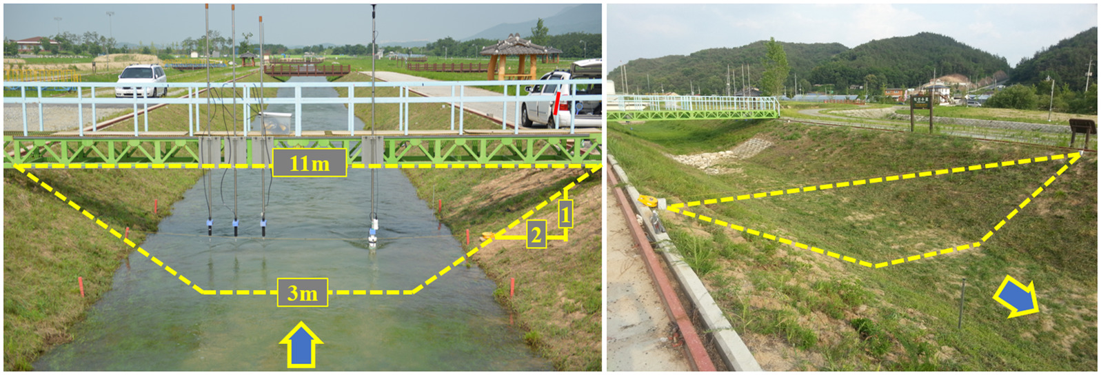
At the time of the experiment, the channel cross section had slightly vegetated channel banks and bottom growing on a coarse sand substrate. The bed was stable during the experiments as shown by the pre- and postsurveys of the cross section in the test area. Essential aspects of the facility and flow conditions for the case study are provided in Tables 1 and 2, respectively. The three SonTek microADVs used in the study were installed on mobile traverse set across the channel, as shown in Fig. 5. Velocities in points were acquired with an ADV attached to a mechanically operated rod with finest graduation of 0.0008 m. The ADV data were acquired in 208 fixed locations arranged in a preestablished grid, shown in Fig. 4. The distance between the verticals was 0.25 m to ensure a high-density of measurements across the stream section for a robust estimation of the reference discharge and good sample for testing the sensitivity of the uncertainty associated with the number of verticals. This spacing also ensures that each panel conveys less than 10% of the total discharge as recommended by ISO 1088 (ISO 2007b) standard. The overall duration of the experiment was 32 h. The flow steadiness and uniformity were tracked 9 h before the experiment and over the whole duration of the experiment with dedicated sensors (Kim et al. 2018).
| Channel descriptor | Details |
|---|---|
| Configuration | Straight |
| Cross section | Trapezoidal |
| Bed slope | 0.00125 |
| Length | 560 m |
| Boundaries | Vegetated |
| Test section | 470 m (from entrance) |
| Max. discharge |
| Variable | Value |
|---|---|
| Discharge | |
| Channel width | 6.5 m |
| Averaged velocity | 0.56 m |
| Maximum velocity | 0.89 m |
| Averaged depth | 0.61 m |
| Maximum depth | 0.85 m |
| Aspect ratio | 10.72 |
| Reynolds number | 308,209 |
| Froude number | 0.23 |
Given that UA studies require a reference for uncertainty evaluations, a benchmark for the study was created. Ideally, such a benchmark should be acquired with a high-quality instruments different from the ones subject to UA. The controlled measurement environment offered by the KICT-REC facility equipped with high-precision, high-resolution instruments, and well-established measurement protocols, offers favorable conditions for the creation of a benchmark data set that is close enough to being considered as reference for uncertainty assessments. A similar approach is used by Bertrand-Krajewski et al. (2021).
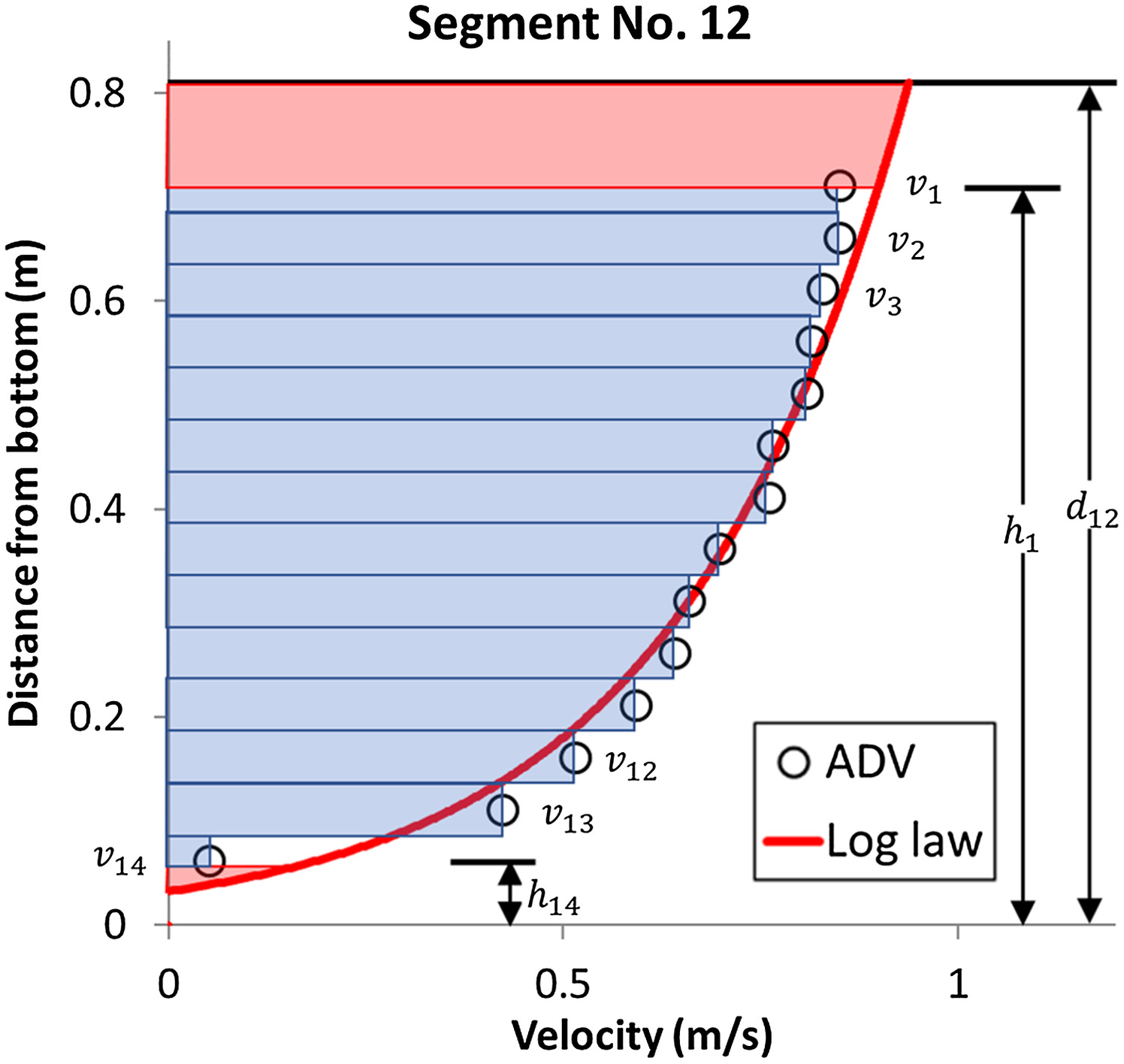
Taking advantage of the high-spatial density of ADV velocities, the mean streamwise point velocities acquired over 90-s sampling duration (Muste et al. 2021) could be reliably extrapolated to the top and bottom of the vertical using a logarithmic (or similar) velocity model applied to all the ADV measurements in individual verticals. For our case, the “reference” velocity distribution is the “log law,” as illustrated in Fig. 6 for vertical #12. Assuming negligible integration errors, the equation for the regression lines in each vertical is considered as reference velocity. Using log-law velocity profiles in verticals #1 to #23, the cross-section geometry surveyed by multiple methods (see section on the depth instrument accuracy in the Appendix), and the edge discharge obtained with additional measurements in the edge areas (Kim 2021; Muste et al. 2021) enabled to determine the “reference” discharge reported in Table 2.
Identification and Evaluation of Elemental Uncertainty Sources
Table 3 provides the summary of the identified uncertainty sources and their estimates as documented by direct measurements conducted in the case study (Type A) or prior knowledge and expert judgement (Type B). The previous standards [especially ISO 748 and ISO 1088, also referred to in HUG (ISO 2020)] are helpful in providing some of the Type B elemental uncertainties. Short descriptions for individual error sources and considerations on the estimates are provided in the Appendix. Type A uncertainty estimates contained in Table 3 were obtained through three repeated field measurement campaigns carried out in the Andong experimental channel, each lasting more than 30 h. The flow conditions for the repeated measurements were practically the same, with discharge differences less than 7%. The small difference between the bulk flow parameters for various experiments ensures that the values of estimated uncertainties are transferable among the three experiments. During the uncertainty assessments, it was aimed at capturing the effect of the individual uncertainty sources acting in isolation, hence qualifying for the “freezing” approach desired in the evaluation of the individual sources of errors.
| Elemental uncertainty | ID | Type | Standard uncertainty | Dependencies | Estimation considerations | References | ||
|---|---|---|---|---|---|---|---|---|
| Source | Divisora | |||||||
| 1. Mean velocity in verticals, | ||||||||
| Instrument accuracy | B | 1.0%b | F(ADV model, flow, operations) | End-to-end calibration | Normal | 2 | Lemmin (2017) | |
| Sampling duration | A | 0.7% | F(flow, instrument settings) | Fig. A1 for 90-s | Normal | 2 | Muste et al. (2021) | |
| Vertical sampling model | A | 1.6% | F(# of points, flow depth, integration type). Include , | Fig. A2 for & 12 verticals | Normal | 2 | Kim et al. (2018) and ISO 748 (ISO 2007a) | |
| Vertical velocity model | A | 0.3% | F(flow depth, turbulence intensity, roughness). Include , | End-end-calibration | Normal | 2 | Kim et al. (2018) | |
| Correlated bias errors | — | N/A | Point-velocities measured with same instrument | N/A | — | — | JCGM 100 (JCGM 2008a) | |
| Operational conditions | A | Negligible | F(instrument, operations, environment) | Expert knowledge | -Student | 1 | Kim (2021) | |
| 2. Depth in verticals, | ||||||||
| Instrument accuracy | B | 0.0005 m | F(instrument settings and siting, site conditions) | Instrument resolutionc | Rectangular | 1.73 | Kim (2021) | |
| Correlated bias errors | — | N/A | Depths measured with same instrument | N/A | — | — | JCGM 100 (JCGM 2008a) | |
| Operational conditions | A | Negligible | F(instrument, operations, environment) | Expert knowledge | — | — | — | |
| 3. Distance between verticals, | ||||||||
| Instrument accuracy | B | 0.0005 m | F(instrument settings and siting, flow conditions) | Instrument resolutionc | Rectangular | 1.73 | — | |
| Correlated bias errors | — | N/A | Distances measured with same instrument | N/A | — | — | JCGM 100 (JCGM 2008a) | |
| Operational conditions | A | Negligible | F(instrument, operations, environment) | Expert knowledge | — | — | WMO (2010) | |
| 4. Discharge model, | ||||||||
| Discharge model | B | 0.5% | F(discharge model, density of velocity points) | End-to-end measurements | Normal | 2 | Muste et al. (2004) | |
| Number of verticals | A | 1.5% | F(discharge model, cross-section geometry) | Fig. 14 for 12 verticals & | Normal | 2 | Kim et al. (2018); Le Coz et al. (2012); Despax et al. (2016a); and ISO 748 (ISO 2007a) | |
| Edge discharge model | , | A | 1.7% | F(discharge model, edge shape) | End-to-end measurements | -Student | 1 | Kim et al. (2018) and HUG (ISO 2020) |
| Operational conditionsd | B | Negligible | F(instrument, operations, environment) | Expert knowledge | — | — | WMO (2010) and HUG (ISO 2020) | |
a
The divisor is the value by which the standard uncertainty is divided to obtain the standard deviation for the probability distribution assumed for the th source of uncertainty.
b
Relative uncertainty estimated estimates are converted to absolute (dimensional) values during the propagation process.
c
Estimated as half of the instrument resolution assumed as a rectangular distribution.
d
This source of uncertainty does not include operational uncertainty sources associated with uncertainty sources listed above to avoid double counting.
Type B uncertainties were selected from various sources as specified in the last column of Table 3. All these data sources were deemed rigorous with respect to uncertainty assessment procedures. However, given that the information on some elemental uncertainty might be different in various sources, critical judgement was used to select estimates that are most relevant to our specific measurement situation. The elemental uncertainties associated with each group are aggregated using the root-sum-square (see Step 2 in Fig. 1) to obtain the standard uncertainty for each variable in Eq. (6).
There are several notable aspects about the information contained in Table 3, as follows:
•
The instrument accuracy for the measurement of the variables in the functional relationships [Eq. (5)] is estimated without accounting for improperly reported calibration data, sensor drift, or inappropriate instrument maintenance or operations. Given that these latter aspects are instrument and situation specific (i.e., measurement environment and instruments’ operations), they are included in the operational conditions category that is associated with all the uncertainty sources.
•
Care was taken to avoid double counting of the same source of uncertainty in more than one group, with special attention to operational conditions sources that are affecting all uncertainty groups.
•
The distribution of the sample measurements for estimation of the individual uncertainty sources is usually assumed to be normal (i.e., Gaussian) if not otherwise noted. Estimation of other forms of probability distributions (i.e., rectangular, triangular, or trapezoidal) requires specialized tests that are difficult to obtain in field conditions due to the variability of the measurement environment.
•
The standard uncertainties for the elemental uncertainty sources are assumed to be derived from large enough statistical samples, hence having an infinite degree of freedom. Strictly speaking, a large sample from statistical considerations would imply to acquire more than 30 repeated measurements (for avoiding the use of Student distribution for the determination of the coverage factor, ). However, many uncertainty estimates are obtained from samples of less than 10 repeated measurements because obtaining larger samples is too expensive, or quite impossible, to gather when confronted with the natural flow variability during the measurement process.
•
Estimation of the coverage interval for the reported uncertainties is given for a 95% confidence level with a coverage factor of .
Estimation of Total (Expanded) Uncertainty in Discharge Measurement
The total uncertainty of the discharge using the ADV point-velocity measurements is obtained following the algebraic calculations shown in Steps 3 and 4 of Fig. 1. The total uncertainty (expressed by the combined uncertainty) in the flow discharge is obtained with Eqs. (6) and (7) using a coverage factor of . The combined uncertainties associated with the main measured variables (mean velocity in the verticals, , depth in verticals, , distance between verticals, , and with the discharge estimation model, , are aggregated through the following relationships:
(8)
(9)
(10)
(11)
Notations and essential specifications for all elemental sources of uncertainties are provided in Table 3 and the Appendix, respectively. Noting the absence of estimates for the correlated uncertainties in Table 3, the corresponding terms in Eq. (6) are also dropped in the evaluation of the uncertainty for the final result.
The calculation of the total discharge and the propagation of the elemental uncertainties generated in the measured and unmeasured areas of the cross section were conducted using the QMsys Enterprise (Qualisyst 2019). A dedicated interface, labelled QMSys Calculator (Qualisyst 2019), was used for providing the functional relationship and the values for elemental uncertainties in Table 3. This GUM-compliant software is executing Step 3 in Fig. 1 using interactive graphical user interfaces (GUI) that aid users with the data reduction process, as well as visualizing the UA results and summaries in a user-friendly format (Muste and Lee 2011). The software is initiated by typing in the software Eq. (5) for the functional relationship of the measurement process. Eqs. (6) and (7) are numerically determined by the software. A confidence level of 95% was uniformly applied to the elemental sources and total uncertainty.
The QMsys Enterprise software is also capable of estimating uncertainties in results using the MCM, an approach often used as a means of “validation” for the GUM conventional method (Bertrand-Krajewski et al. 2021). The reason for choosing MCM as reference is that it does not require special provisions for Type B of uncertainties. If both methods produce close results using the same inputs for the variance of elemental sources of uncertainties, then the law of propagation of uncertainty can be applied, which may be more convenient, especially with repetitive calculations. If the results are not equivalent, then the MCM should be used (Bertrand-Krajewski et al. 2021). The results of the QMsys produced for this case study obtained with the GUM protocol for propagation of variances (labelled GUF in the software) and MCM simulations are shown Table 4.
| Assessment method | Number of trials (M) | Estimated mean () () | Combined standard uncertainty [] () | Expanded standard uncertainty (95% confidence interval) | Numerical tolerance, | GUF validated | |||
|---|---|---|---|---|---|---|---|---|---|
| () | (%) | ||||||||
| GUF | n/a | 2.048 | N/A | N/A | N/A | N/A | |||
| MCM | 2.048 | 1.981 | 2.115 | 3% | Yes | ||||
Note: GUF = GUM uncertainty framework.
The graphical comparison of the two GUM-complaint approaches is illustrated in Fig. 7. The data in the table illustrate that the expanded standard uncertainties estimated by the conventional GUM and MCM are in good agreement. The MCM validation, with respect to the GUM uncertainty framework (GUF), was also verified by calculating a tolerance interval. An absolute difference between the endpoints of the two coverage intervals ( and in columns 7 and 8 of Table 4) is less than the numerical tolerance value for in column 9, leading to the conclusion that GUF estimated was validated for this case study.
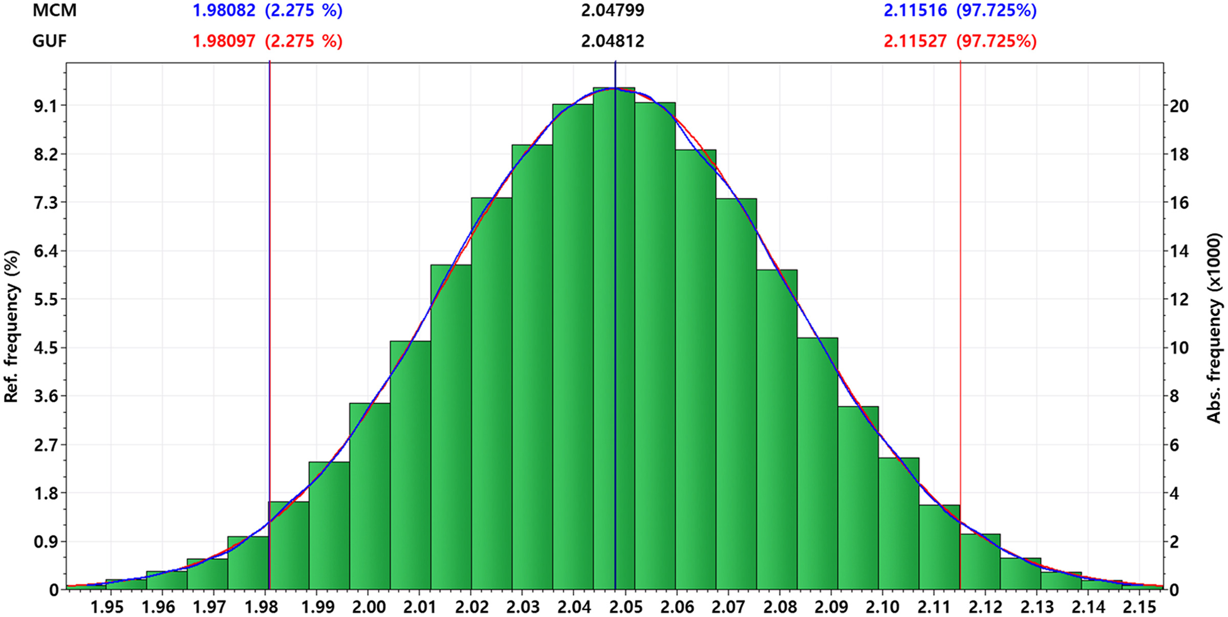
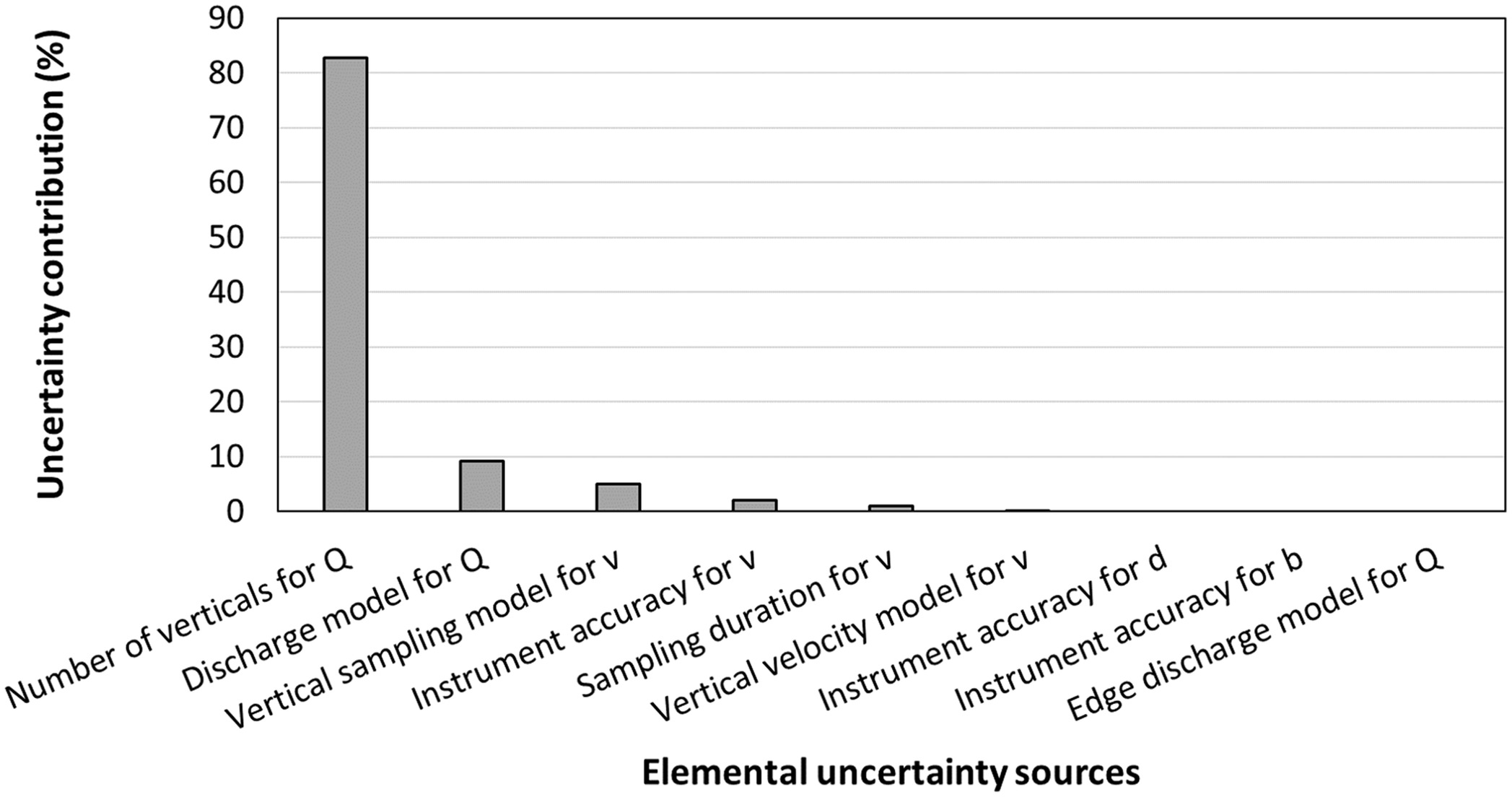
The value of 3.28% for the expanded uncertainty of the measured discharge (estimated at 95% confidence level) is well within the 5% value stated as the acceptable uncertainty for qualifying a measurement of satisfactory quality. However, given the overall good quality of the experiments (i.e., flow in the facility, measurement environment, instruments, and controlled execution of the experiments), the value of the expanded uncertainty may be deemed as large considering that, at natural-scale sites, multiple uncertainty sources may be simultaneously present that can easily exceed the 5% accepted threshold for discharge estimation. Another important UA outcome is the uncertainty budget illustrated graphically in Fig. 8. The uncertainty budget plays multiple roles if the identification of the uncertainties considered in the analysis is complete (see the “Discussion” section).
Discussion
Ignoring UA is no longer a choice for data producers, as data users increasingly call for confidence that the measured data can stand comparisons across agencies as well as scientific and legal scrutiny (Pappenbergen and Beven 2006). Special attention is given to the estimation of the uncertainty for streamflow measurements, one of the most critical variables for water resources and water-hazard forecasting. The analysis presented in the previous section along with the data provided in the Appendix illustrate a realistic implementation of the GUM-based UA protocol in quasi-natural measurement environment using elemental sources of uncertainty determined from our own and previous experiments. We realize that the presented case study is not typical for routine in situ discharge measurements where many of the measurement procedures cannot be executed as straightforward as described herein. While the implementation results are valid only for the conditions of the presented case study, the UA illustration offers suggestions on how the GUM framework can be implemented to other hydrometric measurements. Some lessons learned and hints inferred from the present and previous uncertainty analyses conducted by these authors are highlighted below.
GUM UA Is Doable
This paper, as well as previous case studies conducted by the authors in open-channel flows (e.g., Muste and Lee 2011; Muste 2017b; Muste et al. 2012, 2021) and in urban drainage and stormwater management systems (e.g., Bertrand-Krajewski et al. 2021), illustrate that the full-fledged GUM-UA framework can be executed if proper resources are secured. These illustrations highlight the capability of the framework to adapt to diverse measurement situations, including typical streamflow measurements. While the results of the study are not readily usable for typical in situ measurements, the contribution of this study is identification of the sources of uncertainties and reporting details on how uncertainties at all levels are rigorously estimated as specified by rigorous protocols.
The analysis conducted in this study highlights that the execution of UA requires not only a robust understanding of the UA fundamentals, but also cross-disciplinary knowledge on the flow-related and instrument-sensing processes, instrument configuration and components, and measurement methods and their execution in various environments. Typically, these areas are mastered by different specialization areas or sub-areas, therefore collaboration among various actors is paramount. This paper also demonstrates that the burdensome UA computations are rapidly being (more than) compensated for by the availability of computer processing power. Currently, there are more than 50 GUM-compliant software packages available (Muste 2017a).
Selecting and implementing a generic UA framework such as GUM in the practice of a professional community are actions that require long-term commitment and effort. This paper, ensuing from more than a decade of sustained effort to adopt UA in hydrometry, intends to provide readers with an overview of the benefits of using a judiciously selected UA framework and demonstrating that it can be successfully applied for assessment of measurement uncertainty. According to Thomas (2002), the following steps are essential in the adoption of a community standard: evaluation, prioritization, implementation, planning, accessing various resources, and maintaining the drive. The effort made by the WMO’s Project, “Assessment of the Performance of Flow Measurement Instruments and Techniques,” is an example in this regard (Pilon et al. 2010). Similar efforts are emerging in other water-related communities (Wahlin et al. 2005; Bertrand-Krajewski et al. 2021).
UA Brings a Suite of Benefits
Besides its main role of quantifying the quality of the data, UA implementation can bring several additional benefits (e.g., NAP 2013; Kline 1985). Convincing arguments by McMillan et al. (2017) reveal the critical roles played by UA in water management applications (from reducing project costs to making robust and publicly acceptable decisions at a time of increased uncertainties produced by stresses on water resources from natural and human-induced causes). It is beyond the scope of this paper to detail all these benefits. Instead, we will focus on UA benefits ensuing from the present analysis.
1.
Improving the measurement process and its outcome. The first illustration of the benefits of the present UA analysis is the uncertainty budget output by the UA analysis via the law of propagation of uncertainty (see Fig. 8). This budget reflects the percentage contribution of each term to the sum under the square root in Eq. (6). Similar budgets obtained with MCM are reported in Moore et al. (2016) and Díaz Lozada et al. (2023). These illustrations are powerful tools for all actors involved in the measurement process, from instrument manufacturer to instrument operators and managers of streamflow data. The uncertainty budget offers a synoptic view of all aspects of the measurement process and suggests optimization measures and their order of priority. The uniform and rigorous application of the UA methodology through controlled experiments, such as those reported here, are also helpful to evaluate how a new instrument or discharge measurement method performs in similar or different conditions.
2.
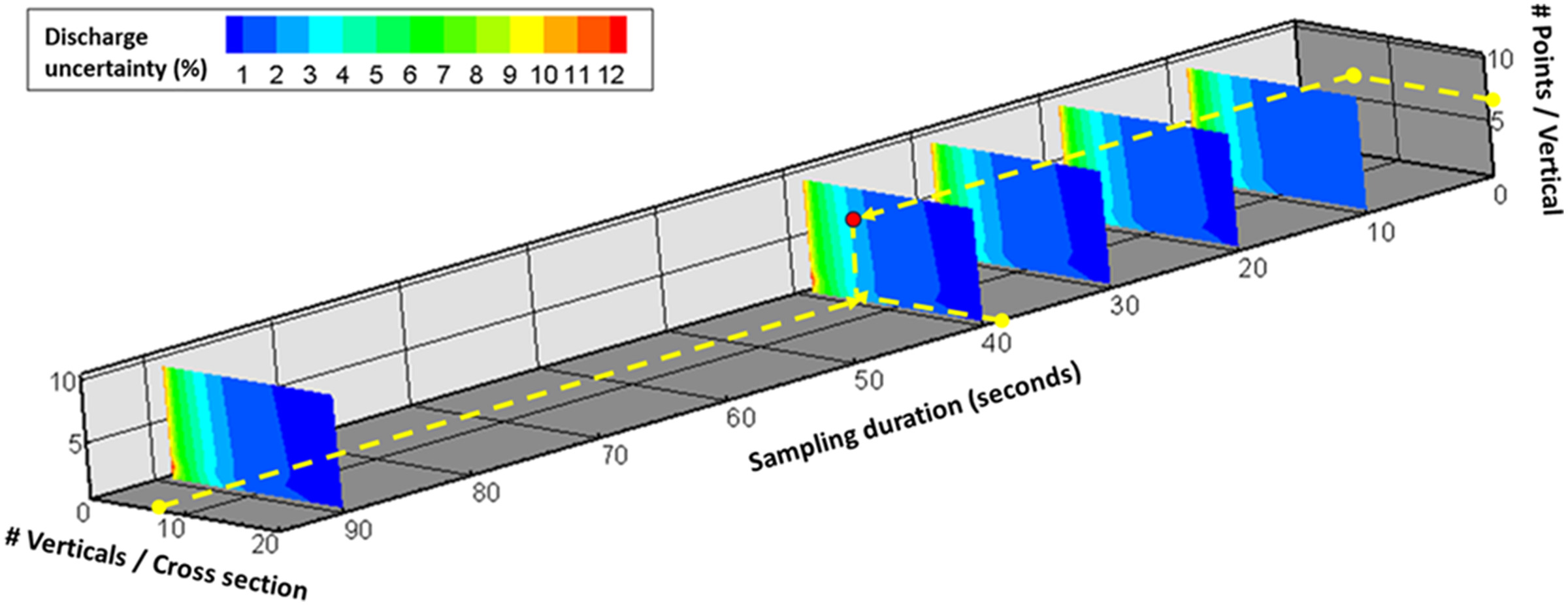
Informing the strategy for the measurement process. The second benefit illustration refers to several sources of uncertainty directly dependent on the operator’s actions. Specifically, sensitivity analysis was conducted to test the impact of operator choices on uncertainty in the depth-average velocity, (directly influenced by selection of the number of points in the verticals and of the sampling duration for each point-velocity measurement), and on the uncertainty in the number of verticals (directly influenced by the selection and distribution of the verticals for acquiring individual point velocities). The description of the uncertainty sources and their estimation is provided in the Appendix. By varying the operator’s options over a range of scenarios, dependencies were created for the impact of the elemental uncertainties , ), on the total discharge uncertainty as illustrated in Fig. 9. The synthetic illustration presented in Fig. 9 suggests that most of the attention for new discharge measurements with point velocities should be given to the number of verticals sampled over the cross section rather than to the sampling duration or the number of points acquired in verticals. This easy-to-understand illustration can unquestionably enhance the strategies to conduct measurements with VA method by helping operators to weigh in on various options and identify the best strategy for the time and resources they have at hand prior to measurement execution.
The ranges of variation for the three uncertainty sources plotted in Fig. 9 are strictly valid for measurements with micro-ADV acquired in turbulent channel flows similar to those tested in the KICT-REC experiments (i.e., streams of similar aspects ratios without prominent changes in the boundary geometry). It should be noted that these uncertainty ranges are slightly narrower and sensibly lower than values currently provided in the ISO 748 (ISO 2007a) hydrologic standard. These differences are due to the highly favorable measurement environment, the superior capabilities of the instrumentation, and the careful measurement design and execution in the KICT-REC case study in comparison with those typically encountered in field studies. From this perspective, it can be stated that the uncertainty estimates illustrated in this study are closer to the lower range of the uncertainties for this kind of measurements. The insights of the above evaluations are, however, valid for other in situ measurements with the VA method. The information is particularly important because the guidelines for sampling point velocities across the section vary widely among various national hydrometric agencies (Le Coz et al. 2012; Despax et al. 2016b).
GUM UA Practicality
The present embodiment of the GUM framework applied to a set of experiments conducted with acoustic point-velocity meters and VA method highlights the complexity required for implementing GUM or any rigorous UA method. This realization is noted upfront in the HUG (ISO 2020): “For practitioners of hydrometry and for engineers, the GUM is not a simple document to refer to” as the framework was developed by professionals with a working knowledge of statistical and mathematical backgrounds. The one-time analysis presented here for one measurement method and one instrument makes it also obvious that UA can easily exceed the resources available for a typical hydrometric project. Additional costs are incurred to implement such analyses within routine data acquisition and training personnel programs of the monitoring agencies.
UA implementation for practical situations is a long-term target due to cost, complexity of uncertainty assessments, institutional resistance, and the additional data acquisition and processing procedures needed (e.g., customized experimental protocols, tools for processing and storing data). Notable progress along the UA technical side is the release of the HUG (ISO 2020) guide that strives to adapt the GUM framework for practical needs of hydrometric engineers and data managers. Further efforts for changing the UA implementation paradigm rely on: (1) providing UA implementation examples using data from routine hydrometric measurements; (2) sharing the data relevant to UA in well-structured databases to enable access to the much-needed Type B uncertainty evaluations; and (3) developing computational and operational tools embedded in software packages that are readily operable by users not familiar with the UA framework.
Adopting UA Requires Concerted Community Efforts
The pressing need to include UA in practice in the hydrometric communities is partially due to a bewildering proliferation of uncertainty methods published in the literature (e.g., Hall and Solomatine 2008; Kiang et al. 2009). Ideally, a unique procedure applied across a wide variety of instruments and methods is preferable to using multiple specific methodologies. One such procedure is the GUM framework. Attaining this target requires coordinated efforts to rally around generic and rigorous UA protocols and making concerted community efforts for their adoption and gradual implementation. Community and individual trainings are needed to fill the gaps in the required UA knowledge (Coelho et al. 2019) and to converge on how to conduct UA in a more practical manner that enables addition of UA when taking in situ measurements. At this time, however, the data necessary for UA are not always available, so new data collection campaigns (perhaps including time-consuming expert elicitation exercises) may need to be commissioned (Hall and Solomatine 2008). Given the high cost of the UAs, data exchange and sharing are essential for community adoption and sustained UA implementation. The data archiving and exchange should be sensitive to all parties involved with the data: producers, providers, and users [see Chapter 10 in Bertrand-Krajewski et al. (2021)].
Conclusion
Streamflow data are typically provided without accompanying uncertainties under the motivation that UA is arduous and expensive. However, the lack of uncertainty on the data raises concern about the reported results and all the derived information that are drawn upon that data. While the instruments, measurement and uncertainty quantification methodologies have advanced and are quite mature at this time, practical UA implementation is lagging because of the lack of convergent guidance and implementation examples. The following contributions of this work are aimed to fill this knowledge-action gap by:
1.
Illustrating the implementation of the widely accepted GUM uncertainty analysis framework to the streamflow measurement through a step-by-step description.
2.
Identifying and assessing with customized experiments some of the sources of uncertainty active in a natural-scale measurements and suggesting practical approaches to circumvent the expensive estimation of uncertainties at the individual variable level.
3.
Discussing the uncertainty analysis results and the benefits brought by it.
To the best knowledge of the authors, this is the first published account of a detailed GUM implementation for discharge measurements with ADV measurements. While the presented example is meant to be generic, we realize that much more such examples are needed to upscale the implementation of uncertainty analysis for in situ measurements.
This paper demonstrates that, although analysis using rigorous UA frameworks is a complex undertaking, it is a doable task. Furthermore, the paper points at the high costs of full-fledged UAs, while also demonstrating that their outcomes produce multiple benefits that pay back the initial investments by leading to more robust and publicly acceptable decisions and reducing the costs of the measurements. Finally, we recognize that UA adoption continues to face resistance. This is quite unfortunate, as there are abundant resources (especially in computer power and communication technologies) that can support a more accelerated UA adoption. This paper calls for community convergence and commitment toward making uncertainty analysis a standard practice for the hydrometric profession.
Appendix. Assessment of the Elemental Error Sources
Provided below are short descriptions and estimates for the standard uncertainties associated with the variables involved in the discharge determination using velocity-area method and ADV point measurements. We organize the discussion of the uncertainties using the following variable grouping:
•
depth-averaged velocity, , that includes uncertainties associated with and
•
depth of the verticals,
•
distance between verticals,
•
model for discharge calculation,
•
model for the edge discharge calculation, and
The estimation of the uncertainty sources is succinctly described one-by-one providing sufficient and clear information for making possible the replication of the estimations such that updates can be made when new data or information become available.
Depth-Averaged Velocity in Verticals,
Instrument Accuracy,
The quality of the ADV measurement is dependent on the presence, density, and size of the particles within the sampling volume that reflect the transmitted signal to the instrument transducers (i.e., backscattering). Sufficient backscatter is an essential requirement for the quality of the acoustic measurement devices (Rehmel 2007). ADVs internally record and report the signal-to-noise ratio (SNR), the standard error of velocity, the angle of the measured flow relative to the axis of the probe, and other parameters that are useful in quantifying the measurement of mean velocity with ADV. Occasionally, incorrect modulation can occur in internal data processing that is not filtered out by instruments. In such occasions, the algorithm proposed by Goring and Nikora (1998) is suggested to be applied in postprocessing before conducting UA. This correction is not common practice in streamflow measurements.
Ideally the estimation of the uncertainty in the mean velocity acquired with ADV should be based on the instrument functional relationship, i.e., Eq. (4), and on the law of propagation of uncertainty (Step 3 in Fig. 1). While the above path is recommended when sufficient resources are available, a more economical alternative for assessing the instrument accuracy is to directly compare the mean velocity acquired with ADV and another instrument previously calibrated at primary standards (Fulford et al. 1999). A sufficiently good instrument is the Pitot tube, a simple and accurate instrument for mean point velocities (Stern et al. 1999). The comparison of the measurements should be done for the range of conditions in the new experiment. Both abovementioned alternative paths are considered Type A evaluations.
Given the limited resources available for the present study, we use a Type B evaluation instead. Fortunately, there are multiple laboratory and field studies documenting that the three components of the flow velocity acquired with ADV are well resolved in a variety of flow conditions (Anderson and Lohrmann 1995; Lane et al. 1998; Voulgaris and Trowbridge 1998). The comparison of a downlooking 10-MHz ADV with a laser doppler velocimeter (a top instrument for velocity measurements) showed 1% difference in the mean velocity (Voulgaris and Trowbridge 1998). The velocity measurement with the ADV might be affected by acoustic interference when the sampling volume is close to (i.e., at about 1 cm near bed or free surface) firm or soft boundaries. We use herein well-maintained ADV probes with an assumed uncertainty of 1% (Lemmin 2017). This value includes the impact of doppler noise and velocity ambiguity; near-sensor phase distortion and averaging over sampling volume; and electronic circuitry noise and A/D conversion. Note is made herein, that the latter impacts are also dependent on the velocity magnitude and turbulence intensity.
Sampling Duration,
There are several studies specifically analyzing the issue of sampling duration in relationship with the quality of the measured velocities with ADV (e.g., MacVicar and Sukhodolov 2019; González-Castro and Lee 2020). The most-often used guidelines for setting the sampling duration for the measurement of mean velocity in channel flows are Table E.3 and Table G.3 for “exposure times” in the ISO 748 (ISO 2007a) and ISO 1088 (ISO 2007b) standards, respectively. These standards were developed to estimate uncertainty of stream discharges determined with the velocity-area method in conjunction with point-velocity measurements acquired with mechanical velocimeters.
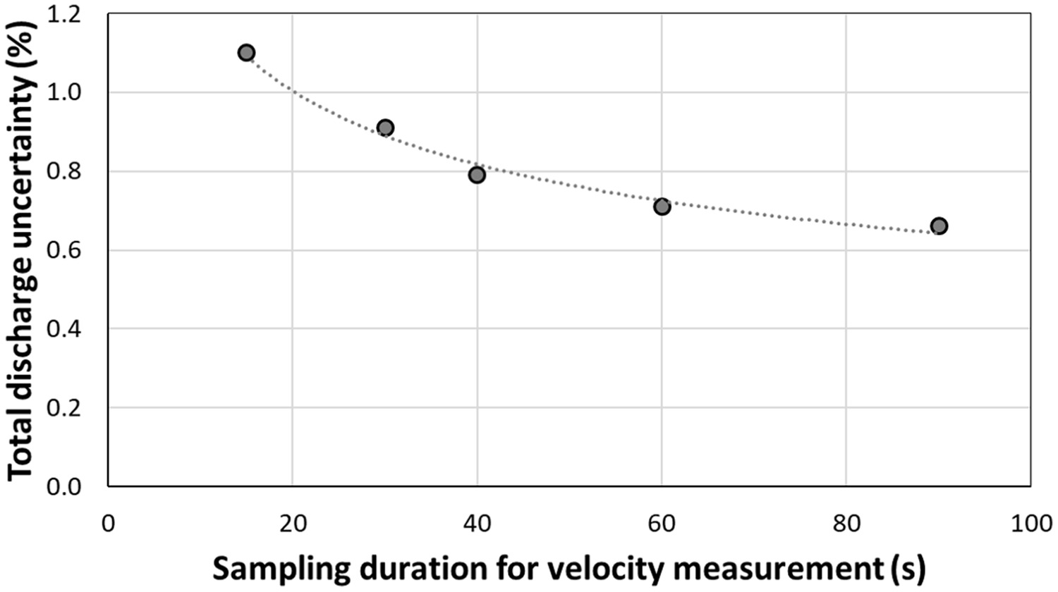
Results of a study conducted at the KICT-REC site to determine the impact on sampling duration for acquiring mean velocities with ADV (acting in isolation) on the discharge values (Type A evaluations) are shown in Fig. 10 (Muste et al. 2017). These estimates are valid for areas away from the stream boundaries. It is expected that the values shown in Fig. 10 are close to the lower bound of the range for this uncertainty source because of the controlled experimental conditions used in the study. More general aspects of the sampling duration in conjunction with the turbulence scales of the flow are provided in Muste et al. (2021).
Vertical Sampling Mode,
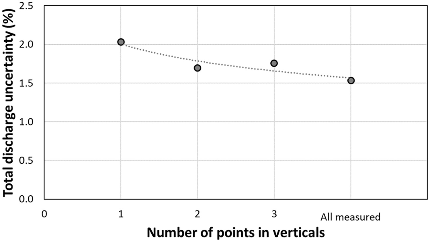
This source of uncertainty is recognized as a major (but not the dominant) contributor to the streamflow uncertainty (e.g., Le Coz et al. 2012). The most-often used sources for this uncertainty are Table E.4 and Table F.1 in ISO 748 (ISO 2007a) and ISO 1088 (ISO 2007b), respectively. These standards offer uncertainty estimates for depth-averaged velocities sampled at 1 to 10 points set at prescribed depths in the vertical (a.k.a., reduced points) with mechanical current meters. However, in practical applications, there are several measurement approaches to obtain the depth-averaged velocities that are not included in these ISO standards. To counteract this limitation, Le Coz et al. (2012) propose a new approach labeled Q+ for estimating the uncertainty associated with both vertical and horizontal sampling. In this approach, the vertical velocity sampling is based on linear interpolation in the measured layer and various extrapolation options in the unmeasured top and bottom layers. Their estimation approach also distinguishes between the method that is used to calculate the discharge (i.e., mid- or mean section). Comparison of ISO 748 with the Le Coz et al. approach shows good agreement for 5 or 6 sampled points (about 2%) but larger differences for lower density sampling (5%–10% for 1–3 points). For the present case study, we take advantage of the high-density point velocities measured at the KICT-REC facility to first obtain a continuous velocity profile (see Figs. 4 and 6) that can be resampled with any number of specified locations (Kim et al. 2018). A sensitivity test to assess the changes in the estimated discharge was done considering 12 verticals sampled with variable number of points, from one point to all acquisition points in the vertical (see Fig. 4). The analysis results applied to the case study are plotted in Fig. 11.
Vertical Velocity Distribution Model,
This type of uncertainty is typically involved when a nonstandard approach is taken to sample point velocities in the vertical. For this situation, recourse is made to a velocity distribution law that is extrapolated in the top and bottom of the vertical, where velocities cannot be measured with the instruments due to the presence of the interfaces. The debate for the most appropriate velocity distribution model in the vertical is a classic topic in open-channel hydraulics (e.g., Nezu and Nakagawa 1993; Guo et al. 2005). It seems that there is a convergence toward adopting log- and power-law for the velocity distribution in the vertical without a final agreement yet on the best approach for all situations. Most probable, each of these distribution laws are better suited for some subclasses of turbulent open-channel flows than for others while the type and the flow range of these subclasses remain still unspecified. Keeping in mind this situation, we took advantage of the dense number of points acquired with ADV for each vertical in our case study to determine the discharge using: (1) the log law; (2) the general power law; and (3) the 1/6 power law (see Fig. 12).
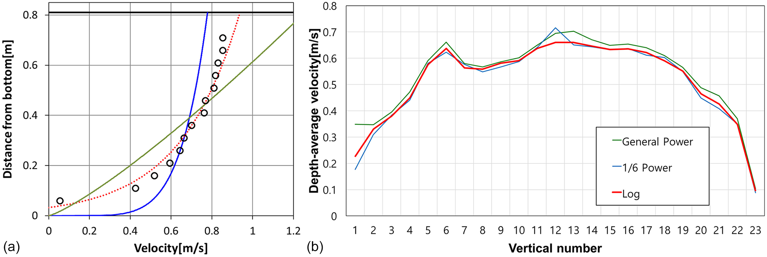
In this analysis, we choose the log-law as reference for the velocity distribution, evaluating the other options against this ad-hoc chosen reference. The input information for estimating the depth-average velocities is uniformly applied for each measured vertical and across all tested distribution laws. The depth used for the analysis is determined from the survey with a total station. Sample comparison of the abovementioned distribution laws for vertical #12 illustrated in Fig. 4 is provided in Fig. 12(a). Fig. 12(b) displays the velocity profiles across the channel section using the distribution laws shown in Fig. 10(a). The numerical results of the impact of choosing various velocity distribution models for estimating the discharge for the present study are provided in Table 5. The present analysis is a typical example of “freezing” approach implementation in the conduct of the uncertainty analysis (i.e., varying one source of uncertainty while keeping all the others the same in the comparison).
| Estimation factor | Log law | Power law | 1/6 power law | 10-pt. method |
|---|---|---|---|---|
| Discharge () | 2.050 | 2.128 | 2.044 | 2.024 |
| Discharge difference () | — | 0.078 | ||
| Uncertainty (%) | — | 3.82 |
Correlated Bias Errors,
Correlations occurring between the variables in the functional relationship of the measurement lead to covariances [JCGM 100 (JCGM 2008a)]. Correlations can be produced by, for example, measuring input quantities with the same instrument or use of the same method for calibration of the instruments [JCGM 100 (JCGM 2008a)]. This is obviously the case for the streamflow measurement relationship where the depth-averaged velocities, depths in the verticals, and distances between verticals for individual subsections (panels) are measured with the same instrument as the measurements progress over the cross section. Another cause leading to correlation between measured velocities in adjacent verticals occurs if the time scale of turbulence is of the same order as the length of time for collecting the measurements in those verticals. Given that the coefficients of correlations may be positive or negative, they may contribute to respectively increasing or decreasing the uncertainty of the respective variable in the total uncertainty budget (Stern et al. 1999; Bertrand-Krajewski et al. 2021).
Detection and quantification of correlations between measured variables (the last term of the equation in Step 3, Fig. 1) are not always obvious and should receive special attention. Correlations between input quantities can be evaluated experimentally by varying the correlated input quantities or by using a pool of available information on the correlated variability of the quantities in question (Bertrand-Krajewski et al. 2021). Currently, we do not have knowledge of customized in situ experiments to assess correlated bias or random errors for streamflow measurements, as these assessments are prohibitively expensive and difficult to conduct in field conditions. Lacking these evaluations, the typical assumption in estimating depth-averaged velocity in verticals is that this random variable is statistically independent with probability distributions identically distributed in each vertical (Cohn et al. 2012). In the present analysis we do not consider this source of uncertainty.
Operational Conditions,
In typical ADV deployment, this elemental source compounds the effects induced by the instrument (e.g., settings of the velocity range, sampling range, temperature, and salinity), operations (e.g., omission or mispositioning of the probe with respect to flows, movement of the wading rod during the measurement), and site conditions at the time of measurements (e.g., temperature, wind, precipitation). Standards do not typically provide information on the uncertainty associated with these factors. A good type of experiment that can benefit the estimation of the operational condition-induced uncertainties is the interlaboratory experiment, where multiple operator teams simultaneously acquire streamflow with the same type of instruments and preestablished protocols (Le Coz et al. 2016; Despax et al. 2016a, 2019). The availability of a facility such as KICT-REC is also appropriate to test and evaluate each of these sources of uncertainty through repeated measurements in which individual sources act in isolation. However, given that the measurement team was well trained, familiar with the instrument setting and operation, and that the measurement environment was not considerably affected by any adverse factors, we do not account for this source of error in the present analysis.
Depth in Verticals,
Instrument Accuracy,
Guidance on standard errors attributable to individual depth measurement errors in discharge measurements are provided in WMO (2010), Table I.10.1. The ISO 748 standard prescribes an uncertainty of 0.65% for range of depths relevant to wading (Table E.2). The stream bed for the present case study was firm with insignificant bed mobility. For the well-controlled conditions in our study, the depths in verticals are determined using the scale attached to the rod on which the ADV was rigidly positioned on the measuring platform. For obtaining the actual depths during the measurements, control points located on the rod and on the mechanical positioning system attached to the bridge along with another set of control points on the channel bed were surveyed with the total station. This procedure allows to determine the actual depths measured from the rod positioned on the platform. Due to the precise setting of all the devices associated with the depth measurements, the positioning is considered free of errors for the present case study.
The choices for the measurement of depth at various locations across the stream (i.e., bathymetry) are multiple, each of them presenting advantages and disadvantages in terms of easiness of measurement, accuracy, the cost of the instrumentation, and of the bathymetric surveys. For the present experiments, the depth across the stream measurement uncertainty is estimated using three alternatives illustrated in Fig. 13: total station (Trimble 5601), staff gauge, and scanning lidar (RIEGL LMS-Z390i). The estimated uncertainties in the discharge using all the point measurements where ADV data was collected, along with the three alternative methods for depth measurements, are shown in Fig. 13.
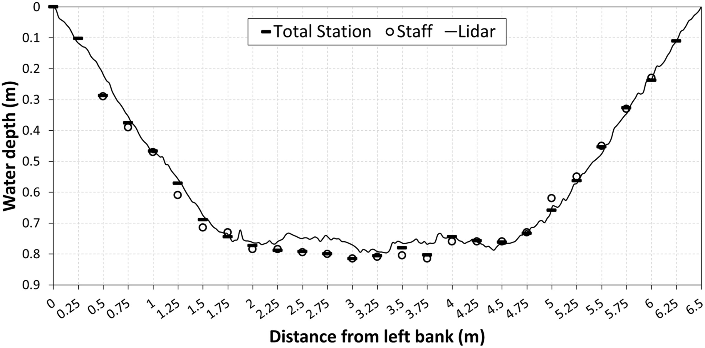
Table 6 provides the summary of the comparison of discharges estimated with depths measured across the stream with the three alternative instruments using the log law for the depth-averaged velocity model. This estimation is another example of the “freezing” approach in the conduct of the uncertainty analysis. For the present analysis we assume that the total station was the most accurate candidate for the bathymetry measurements; hence, we consider the bathymetric depth measurements with total station free of uncertainty. Nevertheless, we include in the analysis the uncertainty associated with the finest resolution on the mechanical positioning vernier (i.e., 0.001 m).
| Estimation factor | Total station | Staff gauge | Lidar |
|---|---|---|---|
| Discharge () | 2.050 | 2.061 | 2.008 |
| Discharge difference () | — | 0.011 | |
| Uncertainty (%) | — | 0.55 |
Correlated Bias Errors,
Similar to the correlated bias errors for point velocities, currently we do not have knowledge of customized in situ experiments for evaluation of the correlated bias or random errors associated with the depth measurements. This source of uncertainty is not considered in the present analysis.
Operational Conditions,
Errors in estimates of the depth of a vertical may occur, from multiple sources, such as positioning the wading rod with varying penetration of the channel bed, difficulty in reading the depth markings on the wading rod, effects of drag on suspension cables and weights, or imprecise reading of the free surface water level in the presence of the inherent water surface. For the present case study, the depth measurements were done with a sturdy mechanical positioning system without bed contact and lack of other detrimental environmental factors. Therefore, we deem that this source of uncertainty is negligible for all measured depths and locations in the verticals.
Distance between Verticals,
Instrument Accuracy,
There are several recommended methods for measuring distances between verticals (see ISO 748, Annex B). Values of 0.5% are prescribed for this uncertainty in ISO 748 and ISO 1088 Table E.1 and Table G.1, respectively. If the uncertainty values cannot be attained, better techniques or procedures should be employed. In our case, the distance from a reference point on the fixed platform to the location of the probe-supporting rod is precisely measured with a tape attached to the platform’s rails. Given that the positioning on the rail is done precisely, only half of the resolution of the finest scale on the measuring tape (i.e., 0.001 m) is attributed for this uncertainty source.
Correlated Bias Errors,
Similar to the correlated bias errors discussed for point velocities and depth measurements, we do not have knowledge of customized in situ experiments for evaluation of the correlated bias or random errors associated with the measurement of the distance between verticals. This category of uncertainty is not considered in the present analysis.
Operational Conditions,
For the present study, we deem that this uncertainty source is negligible as the width measurements were acquired by trained operators from a rigid platform fit with robust positioning system and under an overall good environment during the execution of the measurements.
Discharge Model,
Discharge Model for the Measured Area,
There are several options available for the determination of the discharge in subsections and of the total stream discharge, found in Rantz (1982), ISO 748 (ISO 2007a), and WMO (2010). According to the ISO standard, the midsection method used in the present analysis is quite widespread in the hydrometric community. There are no studies known to the authors that document the effect of the method for determining the total discharge. A major difficulty for this assessment is the lack of a well-established traceable discharge measurement method for field conditions. In the absence of systematic studies documenting the effect of the total discharge methods, we use results from a previous study where the difference between different algorithms for the computation of the total discharge were tested (Muste et al. 2004). Based on this study, the standard uncertainty of this source of uncertainty is set at 0.5%.
Number of Verticals,
Multiple studies find that this source of uncertainty is a major contributor to the total uncertainty in the streamflow measurement (e.g., Le Coz et al. 2012; Despax et al. 2016b; Kim et al. 2018). Prescribed estimates for this uncertainty source are given in Tables E.6 and F.2 of the ISO 748 (ISO 2007a) and ISO 1088 (ISO 2007b), respectively. While representing as much as 85% of the total uncertainty, the ISO standards characterize this uncertainty solely based on the number of verticals without addressing their spatial distribution, shape of the riverbed, and cross-sectional flow distribution. The magnitude of this uncertainty source is highly dependent of the measurement site, especially if the channel bed is highly irregular and the measurement verticals are selected at large distance among themselves. The number of verticals has direct implications on the accuracy in the measurement of the depth-averaged velocity and depth measurements in verticals (Le Coz et al. 2012; Kiang et al. 2009). In our discussion, we associate the number of verticals in the uncertainty group, , without considering their effects on velocity and depth measurements to avoid double counting of elemental errors.
With the realization of the importance of this source of uncertainty, several improvements to the ISO 748 (ISO 2007a) methods were developed. The first improvement in the estimation of the number of verticals on the VA midsection approach was developed by Kiang et al. (2009). In this method, labeled the interpolated variance estimator (IVE), an additional correction of the variances for the depth and velocity is accounted for by using a factor derived from the linear interpolation between the verticals adjacent to the one where the correction is applied. Given that IVE is based on statistical analysis applied to directly measured depths and velocities in successive verticals, it is considered as a Type A evaluation method. Le Coz et al. (2012) developed an alternative approach, labeled Q+, whereby they consider additional uncertainties in depths and depth-averaged velocities in verticals attributed to the type of transversal integration of these variables. An additional feature of the Q+ method is consideration of the changes of the transversal bed slope the bed material. The Q+ method was developed for both midsection and mean-section VA methods. A third approach from this category is the flow analog uncertainty estimation (FLAURE) (Despax et al. 2016b). The method consists in subsampling a set of multiple high-resolution point velocity data sets (considered as “references”) acquired in a variety of streams and rivers. The subsampling consists in generating diverse spatial distributions of the verticals with the aim to simulate the possible choices in approaching the streamflow measurements by a typical field operator. A comparison of ISO 748, Q+, IVE, and FLAURE uncertainty estimation alternatives applied to more than 3,000 gages located in a wide range of flow conditions and cross-section geometries reveals that Q+ and FLAURE provide similar values, while the ISO and IVE overestimate the contribution of the number of verticals to the total discharge uncertainties. The uncertainty difference found in the comparison ranges between 3% and 15% with a mean value of 5%.
Taking advantage of the high-resolution sampling for velocity in this case study, the FLAURE method was selected for a Type A estimation of the impact of the number of verticals on the total uncertainty for the discharge estimation. The results of the application of the subsampling protocol developed by Despax et al. (2016b) is shown in Fig. 14. The number of subsamples and the strategy for selecting the verticals are described in Kim et al. (2018). By isolating the effect of the other sources of uncertainty, the differences in the total uncertainty between the reference discharge and subsampled iterations range from 11.8% for 3 verticals to about 1% for 12 or more verticals. Given that the number of sampled points in the vertical and the number of verticals are typically decided by the hydrometrist at the time of the measurement execution, we provide herein a summary of the combined effect of these two sources in Fig. 14. The results provided in this figure also confirm that the uncertainty associated with the vertical sampling is less important than the one associated with the number of verticals over the cross section. The combined effect of the number of points in the vertical and number of vertical in the cross section on the total uncertainty of the discharge indicate that the impact of number of velocity points acquired in the verticals does not exceed 5% if the number of verticals is larger than 6. The impact of this uncertainty decreases dramatically when the number of verticals increases, becoming practically insensitive for more than 10 verticals acquired over the cross section.
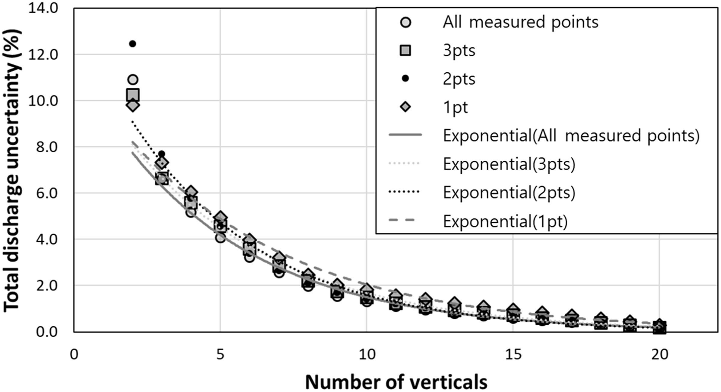
Discharge Model for the Edges, ,
The uncertainty estimation that accounts for the unmeasured areas near the banks takes different forms depending on the discharge estimation algorithm. Most of the proposed methods for edge discharge estimation rely on extrapolations of the velocities measured in the first and last verticals. HUG (ISO 2020) states that the evaluation of the edge discharges as well as those associated with the top and bottom unmeasured areas are problematic, requiring critical thinking when acquiring the data over the measured area and the additional measurements in the unmeasured areas (sometimes with different equipment). This source of error varies widely with the cross-section geometry as well as with the stream aspect ratio (i.e., average width/depth).
There are several published accounts for the estimation of the edge discharge uncertainties (e.g., Fulford and Sauer 1986; WMO 2010; Le Coz et al. 2012). For sloped walls, Fulford and Sauer (1986) assume that the edge is a triangular area extending from the first and last measured verticals to the water edge on both side of the streams. Accordingly, the near-shore discharges are given bywith notation from Fig. 4. The 0.353 coefficient corresponds to a 45-degree angle between the free surface and the sloping bank lines. For other angle values, the coefficient is given by sin (), where is the angle bank angle as defined above. The coefficient becomes, for example, 0.13, 0.25, and 0.42 for angles of 15, 30, and 60 degrees, respectively. Eq. (8) was used for estimating the edge uncertainty with the reference discharges determined from direct measurements collected within edge area (Kim et al. 2018).
(12)
Operational Conditions,
If the guidelines for the acquisition of all measured variables [e.g., ISO 748 (ISO 2007a)] are strictly followed, this uncertainty is small. However, even if all precautions related to discharge measurement are taken, adverse operational conditions add errors. Among these factors are (the list is not sorted by priority) changes of the material in suspensions from section to section, the presence of temporary secondary currents in the cross section, getting outside the instrument measurement range or the preset operational parameter range (e.g., depth, temperature, salinity), loosening of the original tag line position, significant flow disturbance produced by wind, type of platform used for the measurements, presence of moving bed, changes of the operation protocols or other settings of the instruments involuntarily or for undetected reasons, and, the presence or changes in the environmental factors (e.g., rainfall, ice, humidity, solar radiation, etc.). Regarding the latter category, HUG (ISO 2020) prescribes in Table 2 some of the environmental impacts on these types of hydrometric measurements.
There are some atypical effects on the measurement system that are brought to attention herein as they have important implications on the measurement uncertainties. Among them, two have received special attention: the operator skills (i.e., experience level, habitual behavior) and flow unsteadiness. Regarding the operator skills, it was found that the associated uncertainty can be as high as 2.5% for streamflow measurements using current meters (WMO 2017). The second atypical effect is related to the presence of unsteady flow, (i.e., time-variation of the flow), during the data acquisition. Flow unsteadiness can occur due to natural causes (e.g., flood wave propagation) or operations at manmade control structures that trigger transitional regimes that can last from the order of hours to days or even months. As the measurements process can take from minutes to hours, the steady flow assumption can be used if the gradual flow time scale is much longer than the duration of the discharge measurement. Practical guidance offered by ISO 748 standard recommends that the flow can be considered steady if there are no changes of the flow more than 5% over 30 min. If the flow unsteadiness during discharge measurements needs to be accounted for, special procedures for removing its influence are required [e.g., Section 6.2. in ISO 1088 (ISO 2007b); Joannis and Bertrand-Krajewski 2009)].
None of the above conditions were noticed during our case study measurements, as proven by the stability of the flow over 9 h prior to starting the production measurements when the stage and flow uniformity was regularly checked with pressure gages distributed along the experimental channel (see Kim et al. 2018). Given the flow steadiness during these experiments and the lack of other active sources of uncertainties associated with the measurements of velocities and depths in the verticals, we neglect this group of uncertainty for the present analysis.
Data Availability Statement
Some or all data, models, or code generated or used during the study are proprietary or confidential in nature and may only be provided with restrictions. The raw data acquired for the presented analysis were acquired during a KICT internal project and require approval for release, there are no models developed through this study. The uncertainty analysis is conducted with a commercially available software following the GUM protocols. All ADV raw point-velocity data can be shared with the approval of the authors.
Acknowledgments
This work is supported by the Korea Agency for Infrastructure Technology Advancement (KAIA) grant funded by the Ministry of Land, Infrastructure, and Transport (Grant 21DPSC-C163249-01). The first author acknowledges the partial support from the National Science Foundation EAR-HS 2139649 and EAR-ES 2012850 awards.
References
Anderson, S., and A. Lohrmann. 1995. “Open water test of the Sontek acoustic Doppler velocimeter.” In Proc., IEEE 5th Working Conf. on Current Measurements, 188–192. New York: IEEE.
Bertrand-Krajewski, J.-L., F. Clemens-Meyer, and M. Lepot. 2021. Metrology in urban drainage and stormwater management: Plug and pray. London: IWA Publishing. https://doi.org/10.2166/9781789060119.
Beven, K. J., et al. 2017. “Epistemic uncertainties and natural hazard risk assessment. 2. What should constitute good practice?” Nat. Hazards Earth Syst. Sci. Discuss. 18 (10): 2769–2783. https://doi.org/10.5194/nhess-18-2769-2018.
Chiu, C.-L., and Y.-C. Chen. 1998. “A fast method of discharge measurement in open-channel flow.” In Proc., Water Resources Engineering ‘98, edited by Abt, et al., 1721–1726. Reston, VA: ASCE.
Coelho, M., C. V. S. Fernandes, and D. H. M. Detzel. 2019. “Uncertainty analysis in the detection of trends, cycles, and shifts in water resources time series.” Water Resour. Manage. 33 (8): 2629–2644. https://doi.org/10.1007/s11269-019-02210-1.
Cohn, T., J. Kiang, and R. Mason. 2012. “Estimating measurement uncertainty using the interpolated variance method.” J. Hydraul. Eng. 139 (5): 502–510. https://doi.org/10.1061/(ASCE)HY.1943-7900.0000695.
Despax, A., A.-C. Favre, A. Belleville, A. Hauet, J. Le Coz, G. Dramais, and B. Blanquart. 2016a. “Field inter-laboratory experiments versus propagation methods for quantifying uncertainty in discharge measurements using the velocity-area method.” In Proc., RiverFlow 2016, Constantinescu, et al. Boca Raton, FL: CRC Press.
Despax, A., J. Le Coz, A. Hauet, D. S. Mueller, F. L. Engel, B. Blanquart, B. Renard, and K. A. Oberg. 2019. “Decomposition of uncertainty sources in acoustic Doppler current profiler streamflow measurements using repeated measures experiments.” Water Resour. Res. 55 (9): 7520–7540. https://doi.org/10.1029/2019WR025296.
Despax, A., C. Perret, R. Garçon, A. Hauet, A. Belleville, J. Le Coz, and A.-C. Favre. 2016b. “Considering sampling strategy and cross-section complexity for estimating the uncertainty of discharge measurements using the velocity-area method.” J. Hydrol. 533 (Jun): 128–140. https://doi.org/10.1016/j.jhydrol.2015.11.048.
Díaz Lozada, J. M., C. M. Garcia, K. Oberg, T. M. Over, and F. F. Nieto. 2023. “Improvements to estimate ADCP uncertainty sources for discharge measurements.” Flow Meas. Instrum. 90 (Apr): 102311. https://doi.org/10.1016/j.flowmeasinst.2023.102311.
Dombroski, D. E., and J. P. Crimaldi. 2007. “The accuracy of acoustic Doppler velocimetry measurements in turbulent boundary layer flows over a smooth bed.” Limnol. Oceanogr.: Methods 5 (1): 23–33. https://doi.org/10.4319/lom.2007.5.23.
Fulford, J., and V. B. Sauer. 1986. Comparison of velocity interpolation methods for computing open-channel discharge. US Geological Survey water-supply paper, 139–144. Washington, DC: USGS.
Fulford, J. M., K. G. Thibodeaux, and W. R. Kaehrle. 1999. “Comparison of current meters used for stream gaging.” In Fundamentals and advancements in hydraulic measurements and experimentation, 376–385. Reston, VA: ASCE.
Gonzalez-Castro, J., and M. Muste. 2007. “Framework for estimating uncertainty of ADCP measurements from a moving boat using standardized uncertainty analysis.” J. Hydraul. Eng. 133 (12): 1390–1410. https://doi.org/10.1061/(ASCE)0733-9429(2007)133:12(1390).
González-Castro, J., and K. Lee. 2020. “Uncertainty estimates in point-velocity measurements due to exposure time by functions that assimilate ISO-1088 data & statistically based on the time scale of the very-large-scale flow motions.” Flow Meas. Instrum. 71 (Jan): 101676. https://doi.org/10.1016/j.flowmeasinst.2019.101676.
Goring, D. G., and V. I. Nikora. 1998. “ADV measurements of turbulence: Can we improve their interpretation?” J. Hydraul. Eng. 124 (6): 630–634. https://doi.org/10.1061/(ASCE)0733-9429(1998)124:6(630).
GUM. 1995. Guide to the expression of uncertainty in measurement. Geneva: ISO.
Guo, J., P. Y. Julien, and R. N. Meroney. 2005. “Modified log-wake law in zero-pressure-gradient turbulent boundary layers.” J. Hydraul. Res. 43 (4): 421–430. https://doi.org/10.1080/00221680509500138.
Hall, J., and D. Solomatine. 2008. “A framework for uncertainty analysis in flood risk management decisions.” Int. J. River Basin Manage. 6 (2): 85–98. https://doi.org/10.1080/15715124.2008.9635339.
Herschy, R. 2009. Streamflow measurement. London, UK: Routledge.
ISO. 2007a. Hydrometry-measurement of liquid flow in open channels using current-meters and floats. ISO 748. Geneva: ISO.
ISO. 2007b. Hydrometry-velocity-area methods using current-meters-collection and processing of data for determination of uncertainties in flow measurement. ISO 1088. Geneva: ISO.
ISO. 2020. Hydrometric uncertainty guidance. ISO 25377. Geneva: ISO.
JCGM (Joint Committee for Guides in Metrology). 2008a. Evaluation of measurement data—Guide to the expression of uncertainty in measurement (GUM 1995 with minor corrections). JCGM 100. Geneva: ISO.
JCGM (Joint Committee for Guides in Metrology). 2008b. Evaluation of measurement data—Supplement 1 to the guide to the expression of uncertainty in measurement—Propagation of distributions using a Monte Carlo method. JCGM 101. Geneva: ISO.
Joannis, C., and J.-L. Bertrand-Krajewski. 2009. “Incertitudes sur un mesurande défini comme une valeur intégrée d’un signal continu discrétisé en fonction du temps—application aux mesures hydrologiques enregistrées in situ (Uncertainty in a measurand defined as the integrated value of a continuous signal discretised in time, in French).” La Houille Blanche 95 (3): 82–91. https://doi.org/10.1051/lhb/2009031.
Kiang, J. E., T. A. Cohn, and R. R. Mason. 2009. “Quantifying uncertainty in discharge measurements: A new approach.” In Proc., ASCE World Environmental and Water Resources Congress 2009, 5924–5931. Reston, VA: ASCE.
Kim, D., A. Despax, M. Muste, and J. Le Coz. 2018. “Estimation of the critical uncertainty sources in discharge measurements using controlled experimental conditions.” In Proc., River Flow 2018 Conf. Beijing: International Association for Hydro-Environment Engineering and Research.
Kim, J. 2021. “ADCP discharge uncertainty assessment by GUM framework.” Ph.D. dissertation, Dept. of Civil and Environmental Engineering, Dankook Univ.
Kline, S. J. 1985. “The purposes of uncertainty analysis.” J. Fluids Eng. 107 (Jan): 153–160. https://doi.org/10.1115/1.3242449.
Kraus, N., A. Lohrmann, R. Cabrera, and N. Kraus. 1994. “New Acoustic meter for measuring 3D laboratory flows.” J. Hydraul. Eng. 120 (3): 406–412. https://doi.org/10.1061/(ASCE)0733-9429(1994)120:3(406).
Lane, S. N., P. M. Biron, K. F. Bradbrook, J. B. Butler, J. H. Chandler, M. D. Crowell, S. J. McLelland, K. S. Richards, and A. G. Roy. 1998. “Three-dimensional measurement of river channel flow processes using acoustic Doppler velocimetry.” Earth Surf. Processes Landforms 23 (13): 1247–1267. https://doi.org/10.1002/(SICI)1096-9837(199812)23:13%3C1247::AID-ESP930%3E3.0.CO;2-D.
Le Coz, J., B. Blanquart, K. Pobanz, G. Dramais, G. Pierrefeu, A. Hauet, and A. Despax. 2016. “Estimating the uncertainty of streamgauging techniques using in situ collaborative interlaboratory experiments.” J. Hydraul. Eng. 142 (7): 04016011. https://doi.org/10.1061/(ASCE)HY.1943-7900.0001109.
Le Coz, J., B. Camenen, X. Peyrard, and G. Dramais. 2012. “Uncertainty in open-channel discharges measured with the velocity-area method.” Flow Meas. Instrum. 26 (Jun): 18–29. https://doi.org/10.1016/j.flowmeasinst.2012.05.001.
Lee, K., H. C. Ho, M. Marian, and C. H. Wu. 2014. “Uncertainty in open channel discharge measurements acquired with StreamPro ADCP.” J. Hydraul. 509 (Feb): 101–114. https://doi.org/10.1016/j.jhydrol.2013.11.031.
Lemmin, U. 2017. “Acoustic instruments for fine-scale flow measurements, Section 3.2.” In Experimental hydraulics, Volume II, edited by J. Aberle, C. D. Rennie, D. M. Admiraal, and M. Muste. New York: Taylor & Francis.
Levesque, V. A., and K. A. Oberg. 2012. “Computing discharge using the index velocity method.” Accessed July 4, 2024. http://pubs.usgs.gov/tm/3a23/pdf/tm3-a23.pdf.
MacVicar, B. J., and A. N. Sukhodolov. 2019. “Sampling strategies to improve scaling parameter estimates in rivers.” J. Hydraul. Res. 57 (6): 798–807. https://doi.org/10.1080/00221686.2018.1522379.
McLelland, S., and A. Nicholas. 2000. “A new method for evaluating errors in high-frequency ADV measurements.” Hydrol. Processes 14 (2): 351–366. https://doi.org/10.1002/(SICI)1099-1085(20000215)14:2%3C351::AID-HYP963%3E3.0.CO;2-K.
McMillan, H., T. Krueger, and J. Freer. 2012. “Benchmarking observational uncertainties for hydrology: Rainfall, river discharge and water quality.” Hydrol. Processes 26 (26): 4078–4111. https://doi.org/10.1002/hyp.9384.
McMillan, H., J. Seibert, A. Petersen-Overleir, M. Lang, P. White, T. Snelder, K. Rutherford, T. Krueger, R. Mason, and J. Kiang. 2017. “How uncertainty analysis of streamflow data can reduce costs and promote robust decisions in water management applications.” Water Resour. Res. 53 (7): 5220–5228. https://doi.org/10.1002/2016WR020328.
Moore, S. A., E. C. Jamieson, F. Rainville, C. D. Rennie, and D. S. Mueller. 2016. “Monte Carlo approach for uncertainty analysis of acoustic doppler current profiler discharge measurement by moving boat.” J. Hydraul. Eng. 143 (3): 04016088. https://doi.org/10.1061/(ASCE)HY.1943-7900.0001249.
Mueller, D. S., C. R. Wagner, and M. F. Winkler. 2007. “Best practices for measuring discharge with acoustic doppler current profilers.” Accessed July 4, 2024. https://hydroacoustics.usgs.gov/publications/QStandards_COE_Final.pdf.
Muste, M., ed. 2017a. Guidelines for the assessment of uncertainty for hydrometric measurement. Geneva: World Meteorological Organization.
Muste, M. 2017b. “Uncertainty analysis for hydraulic measurements.” Chap. 7 in Experimental hydraulics, Volume I, edited by M. Muste, D. A. Lyn, D. M. Admiraal, R. Ettema, V. Nikora, and M. H. Garcia. New York: Taylor & Francis.
Muste, M., D. Kim, and J. A. González-Castro. 2010. “Near-transducer errors in ADCP measurements: Experimental findings.” J. Hydraul. Eng. 136 (5): 275–289. https://doi.org/10.1061/(ASCE)HY.1943-7900.0000173.
Muste, M., D. Kim, and H.-W. Tsai. 2017. “Impact of the sampling duration on the uncertainty in discharge measurements acquired with acoustic doppler velocimeters.” In Proc., Hydraulic Measurements & Experimental Methods Conf. Reston, VA: ASCE.
Muste, M., J. Kim, and D. Kim. 2021. “Impact of sampling duration on the uncertainty of average velocity measurements with acoustic instruments.” Hydrol. Processes 35 (4): e14125. https://doi.org/10.1002/hyp.14125.
Muste, M., and K. Lee. 2011. “Development of the decision-aid tool. Phase I: Review of the available decision-aid tools for implementation of uncertainty analysis.” In Report to the WMO project assessment of the performance of flow measurement instruments and techniques. Iowa City, IA: Univ. of Iowa.
Muste, M., K. Lee, and J. L. Bertrand-Krajewski. 2012. “Standardized uncertainty analysis for hydrometry: A review of relevant approaches and implementation examples.” Hydrol. Sci. J. 57 (4): 643–667. https://doi.org/10.1080/02626667.2012.675064.
Muste, M., T. Vermeyen, R. Hotchkiss, and K. Oberg. 2007. “Acoustic velocimetry for riverine environments.” J. Hydraul. Eng. 133 (12): 1297–1298. https://doi.org/10.1061/(ASCE)0733-9429(2007)133:12(1297).
Muste, M., K. Yu, J. Gonzalez-Castro, and E. Starzmann. 2004. “Methodology for estimating ADCP measurement uncertainty in open-channel flows.” In Proc., World Water and Environmental Resources Congress 2004. Salt Lake City: Environmental & Water Resources Institute.
NAP (National Academies Press). 2013. Environmental decisions in the face of uncertainties. Washington, DC: NAP.
Nezu, I., and H. Nakagawa. 1993. Turbulence in open channel flows. IAHR monograph. Rotterdam, Netherlands: A. A. Balkema.
Nystrom, E. A., K. A. Oberg, and C. R. Rehmann. 2002. “Measurement of turbulence with acoustic doppler current profilers—Sources of error and laboratory results.” In Proc., ASCE-IAHR Hydraulic Measurements & Experimental Methods Conf. Reston, VA: ASCE.
Pappenberger, F., and K. J. Beven. 2006. “Ignorance is bliss: Or seven reasons not to use uncertainty analysis.” Water Resour. Res. 42 (Apr): W05302. https://doi.org/10.1029/2005WR004820.
Pilon, P., M. Muste, J. Fulford, and C. Caponi. 2010. Developing a framework for the assessment of uncertainty in discharge. Vancouver, BC, Canada: Canadian Water Resources Association.
Qualisyst. 2019. QMSys gum enterprise/calculator user guide, A professional tool for determination of uncertainties in flow measurements. Gabrovo, Bulgaria: Qualisyst.
Rantz, S. E. 1982. Measurement and computation of streamflow. Washington, DC: USGS.
Reader-Harris, M. 2007. “ISO flow measurement standards—Report on the ISO/TC 30 meeting in November 2006.” Flow Meas. Instrum. 18 (3–4): 114–120. https://doi.org/10.1016/j.flowmeasinst.2007.05.003.
Rehmel, M. 2007. “Application of acoustic Doppler velocimeters for streamflow measurements.” J. Hydraul. Eng. 133 (12): 1433–1438. https://doi.org/10.1061/(ASCE)0733-9429(2007)133:12(1433).
Rennie, C., A. J. F. Hoitink, and M. Muste. 2017. Experimental hydraulics: Methods, instrumentation, data processing and management, Volume II: Instrumentation and measurement techniques. Boca Raton, FL: CRC Press.
Sontek. 1997. Acoustic doppler velocitmetry operation manual, firmware version 4.0. San Diego: Sontek.
Sontek. 2017. Acoustic doppler velocimeters(ADVs). San Diego: Sontek.
Stern, F., M. Muste, M.-L. Beninati, and W. E. Eichinger. 1999. Summary of experimental uncertainty assessment methodology with example. Iowa City, IA: Univ. of Iowa.
Thomas, F. 2002. “Open channel flow measurement using international standards: Introducing a standards programme and selecting a standard.” Flow Meas. Instrum. 13 (5–6): 303–307. https://doi.org/10.1016/S0955-5986(02)00053-5.
Turnipseed, D. P., and V. B. Sauer. 2010. Discharge measurements at gaging stations: U.S. Geological survey techniques and methods book, 87. Washington, DC: USGS.
UKAS (United Kingdom Accreditation Service). 2007. The expression of uncertainty and confidence in measurements. UKAS Middlesex, UK: UKAS.
USGS. 1994. A history of the water resources branch, U.S. Geological Survey; Volume I, from predecessor surveys to June 30. Edited by R. Follansbee. Denver: USGS.
Voulgaris, G., and J. Trowbridge. 1998. “Evaluation of the acoustic Doppler velocimeter ADV for turbulence measurements.” J. Atmos. Oceanic Technol. 15 (1): 272–289. https://doi.org/10.1175/1520-0426(1998)015%3C0272:EOTADV%3E2.0.CO;2.
Wahlin, B., T. Wahl, J. A. Gonzalez-Castro, and J. Fulford. 2005. “Task committee on experimental uncertainty and measurement errors in hydraulic engineering: An update.” In Proc., World Water and Environmental Resources Congress. Milwaukee: Environmental & Water Resources Institute.
WMO (World Meteorological Organization). 2010. Manual on stream gauging. Volume I: Fieldwork. Geneva: WMO.
WMO (World Meteorological Organization). 2017. “Guidelines for the assessment of uncertainty for hydrometric measurement.” Accessed July 5, 2024. https://library.wmo.int/viewer/55462?medianame=1097_en_.
WSC (Water Survey of Canada). 2015. Standard operating procedures for under ice discharge measurements using ADCPs. Ottawa: WSC.
Information & Authors
Information
Published In

Journal of Hydraulic Engineering
Volume 150 • Issue 6 • November 2024
Copyright
This work is made available under the terms of the Creative Commons Attribution 4.0 International license, https://creativecommons.org/licenses/by/4.0/.
History
Received: Jul 26, 2023
Accepted: May 20, 2024
Published online: Jul 27, 2024
Published in print: Nov 1, 2024
Discussion open until: Dec 27, 2024
ASCE Technical Topics:
- Acoustics
- Analysis (by type)
- Continuum mechanics
- Data analysis
- Detection methods
- Doppler systems
- Dynamics (solid mechanics)
- Engineering fundamentals
- Engineering mechanics
- Equipment and machinery
- Flow (fluid dynamics)
- Flow measurement
- Fluid dynamics
- Fluid mechanics
- Hydraulic engineering
- Hydrologic engineering
- Measurement (by type)
- Measuring instruments
- Methodology (by type)
- Motion (dynamics)
- Research methods (by type)
- Solid mechanics
- Streamflow
- Uncertainty principles
- Water and water resources
- Water discharge
- Water discharge measurement
Authors
Metrics & Citations
Metrics
Citations
Download citation
If you have the appropriate software installed, you can download article citation data to the citation manager of your choice. Simply select your manager software from the list below and click Download.