Reductions in Hydraulic Conductivity of Sands Caused by Microbially Induced Calcium Carbonate Precipitation
Publication: Journal of Geotechnical and Geoenvironmental Engineering
Volume 150, Issue 2
Abstract
Microbially induced calcite precipitation (MICP) modifies soil behavior and properties through the precipitation of calcium carbonate () in the pore space. It has gained prominence as one strategy for biologically induced soil improvement. This study investigates the effect of MICP on hydraulic conductivity reduction and presents permeability reduction models for MICP-treated sands. Four column experiments, each with a different size of poorly graded sand, were subject to low-concentration equimolar MICP treatments while monitoring hydraulic conductivity reduction and precipitated distribution. Multiple MICP treatments produced homogeneous distributions of and caused a gradual reduction in hydraulic conductivity of 50%–90% until a content of was achieved. The high-resolution X-ray computed microtomography (CMT) and scanning electron microscopy (SEM) imaging reveals that the pore-scale precipitation behavior changes from a contact-cementing pattern in fine sands to a mixed pattern of contact-cementing and surface-coating precipitation in coarse sands as the grain size increases. The Kozeny–Carman type of permeability models appear to well capture the hydraulic conductivity reduction caused by MICP as a function of volumetric pore fraction of . The experimental results presented in this study advance our understanding of the pore-scale precipitation patterns in different sizes of sands and their effect on hydraulic conductivity. Additionally, this study provides unique and reliable hydraulic conductivity data that can be used to develop hydraulic conductivity models for MICP-treated sands.
Introduction
Microbially induced calcium carbonate precipitation (MICP) is a versatile biogeotechnical ground improvement technology being developed for use in geotechnical practice (Mitchell and Santamarina 2005; DeJong et al. 2014, 2022). The MICP process involves microbially urea hydrolysis by bacteria, such as Sporosarcina pasteurii, which produces carbonate ions () from urea (). These released carbonate ions then react with calcium ions () that are separately injected and produce calcium carbonate (), which improves the mechanical stiffness and strength of soils (e.g., Mitchell and Ferris 2006; DeJong et al. 2006; Whiffin et al. 2007; Martinez et al. 2013; Al Qabany and Soga 2013; Cheng et al. 2013; Gomez and DeJong 2017; Choi et al. 2020).
The precipitation of calcium carbonate () crystals induces changes in the mechanical, hydraulic, and thermal properties of soils. Expectedly, precipitation decreases the porosity and hence the hydraulic conductivity of soils (e.g., Whiffin et al. 2007; Martinez et al. 2013; Al Qabany and Soga 2013; Dadda et al. 2019; Gomez and DeJong 2017; Zamani and Montoya 2017). The MICP-driven reduction in hydraulic conductivity may be useful in a variety of geotechnical applications, including infiltration control of soil surfaces, engineered hydraulic barriers, sand dune and wind erosion control, and prevention of infiltration and internal erosion in embankments and dams (Chae et al. 2021; Dadda et al. 2019; Jiang et al. 2017; Jiang and Soga 2017, 2019; Liu et al. 2021), as well as in other engineering practices, such as reducing the permeability of landfill soils and crack healing in architecture and structures made of concrete and stones (De Muynck et al. 2008; Hataf and Baharifard 2020; Kim et al. 2013).
Therefore, prediction and control of the extent of reduction in hydraulic conductivity, , caused by MICP is important when designing a treatment strategy. However, the data in previous literature show controversially wide fluctuations, and often inconsistent trends in the MICP-driven reduction of hydraulic conductivity (e.g., Martinez et al. 2013; Al Qabany and Soga 2013; Gomez and DeJong 2017; Lin et al. 2016; Armstrong and Ajo-Franklin 2011; Choi et al. 2017). For instance, Martinez et al. (2013) reported that an increase in the content () to 4% reduces the hydraulic conductivity by 98%, almost by two orders of magnitude. On the other hand, Dadda et al. (2019) reported that the hydraulic conductivity decreases by only 50% with 4% . This contrasting result with a large variation could be attributable to various reasons, including the nature of the tested soils themselves, bacterial reaction rate, treatment solution formulation, injection procedure, and/or testing device configuration. Furthermore, any bias in the measurement method and heterogeneity in precipitation within specimens, including local clogging, can also produce such variations. Therefore, the extent that the hydraulic conductivity decreases with an increase in remains not fully resolved, which consequently hampers the development of a hydraulic conductivity reduction model for MICP-treated soils.
It is widely recognized that many factors affect pore-scale precipitation patterns, including biochemical conditions, such as density of ureolysis bacteria in soils, chemical concentration of the cementation solution, reaction rate of ureolysis, presence of suspended bacteria, and location of attached bacteria (Hammes and Verstraete 2002; Whiffin et al. 2007; Al Qabany and Soga 2013; Wang et al. 2019a, b), and the physicochemical characteristics of soils, such as grain size, grain shape, presence of clay minerals, and water saturation (Cheng et al. 2013; Nafisi et al. 2018; Tiwari et al. 2021). Nonetheless, the roles of grain size on pore-scale precipitation pattern and its effect on hydraulic conductivity reduction remains poorly identified.
Therefore, this study explores reductions in hydraulic conductivity of sands caused by MICP. Particular emphasis is placed on the effects of grain sizes and pore-scale precipitation patterns. A series of column experiments were conducted, in which the MICP method was used to treat four types of sand columns with different grain sizes ranging from 0.2 mm to 3 mm while monitoring changes in hydraulic conductivity. The observed hydraulic conductivity reductions are then correlated to the pore volume fraction of (), and these reduction trends are compared with several Kozeny–Carman type models. This experimental study used X-ray computed microtomography (CMT) imaging at two different scales: one at the column scale and the other at the pore scale. The column-scale X-ray CMT imaging evaluates the uniformity of precipitation throughout the columns over the course of multiple MICP treatments. The high-resolution pore-scale X-ray CMT imaging examines the effect of host sand grain size on pore-scale precipitation as the post-experiment examination. Finally, discussion on implications to field-scale MICP-based ground improvement practices follows.
Materials and Methods
Sands
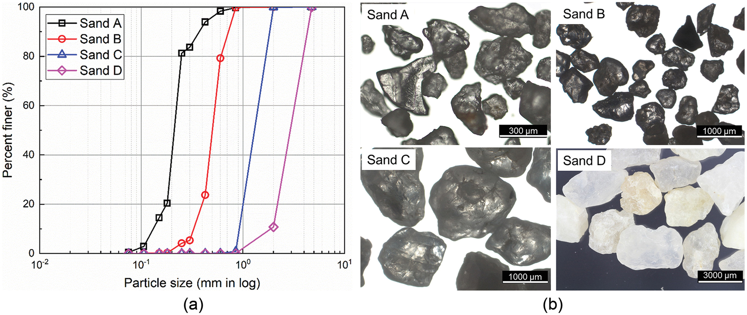
This study used four poorly graded coarse sands, which were sourced from the Cape May Formation near Mauricetown, New Jersey, USA. The formation is known to be interbedded with quartzite sand and gravel containing less than 10% feldspar, and thus the sand is mostly composed of quartz (Owens et al. 1999; Pires-Sturm and DeJong 2022). Table 1 lists the basic index properties of these sands. Fig. 1 shows the grain size distributions and the grain shapes of the test sands. These sands were named Sand A, Sand B, Sand C, and Sand D, as they were the same type of sand but with different gradations. Further material information is available in Pires-Sturm and DeJong (2022). Note that our previous studies in Sturm (2019) and Pires-Sturm and DeJong (2022) also used the same sands, named as 100A, 100B, 100C, and 100D. Sands A, B, C, and D had mean grain sizes, , of 0.21, 0.50, 1.30, and 2.95 mm, respectively, and all were uniformly graded soils with a coefficient of uniformity () of 1.6–1.73. The sands were subangular with a sphericity of 0.63–0.78 and a roundness of 0.36–0.44 (Table 1).
| Parameter | Sand A | Sand B | Sand C | Sand D |
|---|---|---|---|---|
| 2.62 | 2.61 | 2.61 | 2.60 | |
| (mm) | 0.21 | 0.50 | 1.30 | 2.95 |
| (mm) | 0.13 | 0.33 | 0.92 | 2.00 |
| 0.58 | 0.52 | 0.56 | 0.54 | |
| 0.88 | 0.84 | 0.84 | 0.81 | |
| 1.73 | 1.60 | 1.63 | 1.60 | |
| 1.23 | 1.11 | 0.88 | 0.98 | |
| Sphericity | 0.69 | 0.77 | 0.78 | 0.63 |
| Roundness | 0.43 | 0.44 | 0.36 | 0.40 |
Model Bacteria and Treatment Solutions
This study used Sporosarcina pasteurii (ATCC 11859) as the model bacteria, which are capable of urea hydrolysis. Three types of treatment solutions were prepared to culture the model bacteria and stimulate precipitation. The first is the bacterial inoculum solution, which contained the aerobic culture of the model bacteria, . pasteurii, and the fresh growth medium at a volume ratio of . The aerobic culture was prepared by culturing . pasteurii at 30°C under aerobic conditions for until the optical density () reached 1.0. The fresh liquid growth medium contained of yeast extract, of ammonium sulfate, and 130 mM of Tris buffer, following the standard ammonium-yeast extract medium provided by ATCC, and the resulting pH was 8.7. This fresh growth medium was autoclaved at 110°C for 15 min.
The second solution is the rinsing solution, which is comprised of 250 mM of ammonium chloride, 42.5 mM of sodium acetate, and 154 mM of sodium chloride (Gomez et al. 2019; San Pablo et al. 2020). The rinsing solution facilitates the bacterial attachment on sand surfaces while displacing residual suspended bacteria in sand pores, which minimizes local clogging and uneven precipitation in a sand column.
The third is the cementation solution, which consisted of 300 mM of urea, 300 mM of calcium chloride, 25 mM of ammonium chloride, 42.5 mM of sodium acetate, and of yeast extract (Martinez et al. 2013). This solution feeds urea to the bacteria and stimulates the precipitation of minerals by supplying calcium ions. This cementation solution was filter-sterilized prior to injection. Table 2 shows detailed formulations of the solutions used in the column experiments.
| Solution type | Formulation |
|---|---|
| Growth media for S. pasteurii (pH = 8.7) | yeast extract |
| ammonium sulfate | |
| Tris buffer (pH 9.0) | |
| Bacterial solution (inoculum) | 300 mL fresh growth media |
| 30 mL S. pasteurii bacterial culture with | |
| Rinsing solution (pH = 6.0) | 25 mM ammonium chloride |
| 42.5 mM sodium acetate | |
| 154 mM sodium chloride | |
| Cementation solution (pH = 7.0) | 300 mM urea and calcium chloride |
| 25 mM ammonium chloride | |
| 42.5 mM sodium acetate | |
| yeast extract |
Column Setup
A sand pack column with a height of 150 mm and a diameter of 50 mm was prepared in a rigid-walled cylindrical polycarbonate tube, as shown in Fig. 2. There were two pressure ports located along the column length spaced 7 cm apart from each other; these ports were connected to a differential pressure transducer (DPT; PX409, Omega Engineering Inc., Norwalk, CT, USA) to measure the pressure difference between the ports. For Sands C and D, a pair of piezometers were used instead of the commercial DPT due to the high hydraulic conductivities of the sands. Additionally, the pore fluid was sampled from the port at the middle height of the column and the aqueous sample collected was used to monitor the bacterial ureolysis activity through a colorimetric assay (Knorst et al. 1997) and the calcium ion consumption by using an inductively coupled plasma optical emission spectrometer (ICP-OES). Treatment solutions were injected from the bottom at a constant flow rate using a syringe pump (Model 500D, Teledyne ISCO, Lincoln, NE, USA) through a transfer vessel. The springs at the top of the column applied the vertical stress of to prevent any volume change during fluid injections while simulating an effective stress condition at approximately 10 m deep in saturated ground. A pair of bender elements installed at the middle height of the column monitored a change in shear wave velocity, , over the course of the MICP treatment program. In this study, was measured and used as an indicator to monitor the early-stage cementation process. It is because the bender elements were not capable of measuring greater than as the cemented sands around the source bender elements became too stiff to vibrate. Instead, the final values were measured by using free-free resonant column (FFRC) methods after removing the specimens from the columns (Kim et al. 1997).
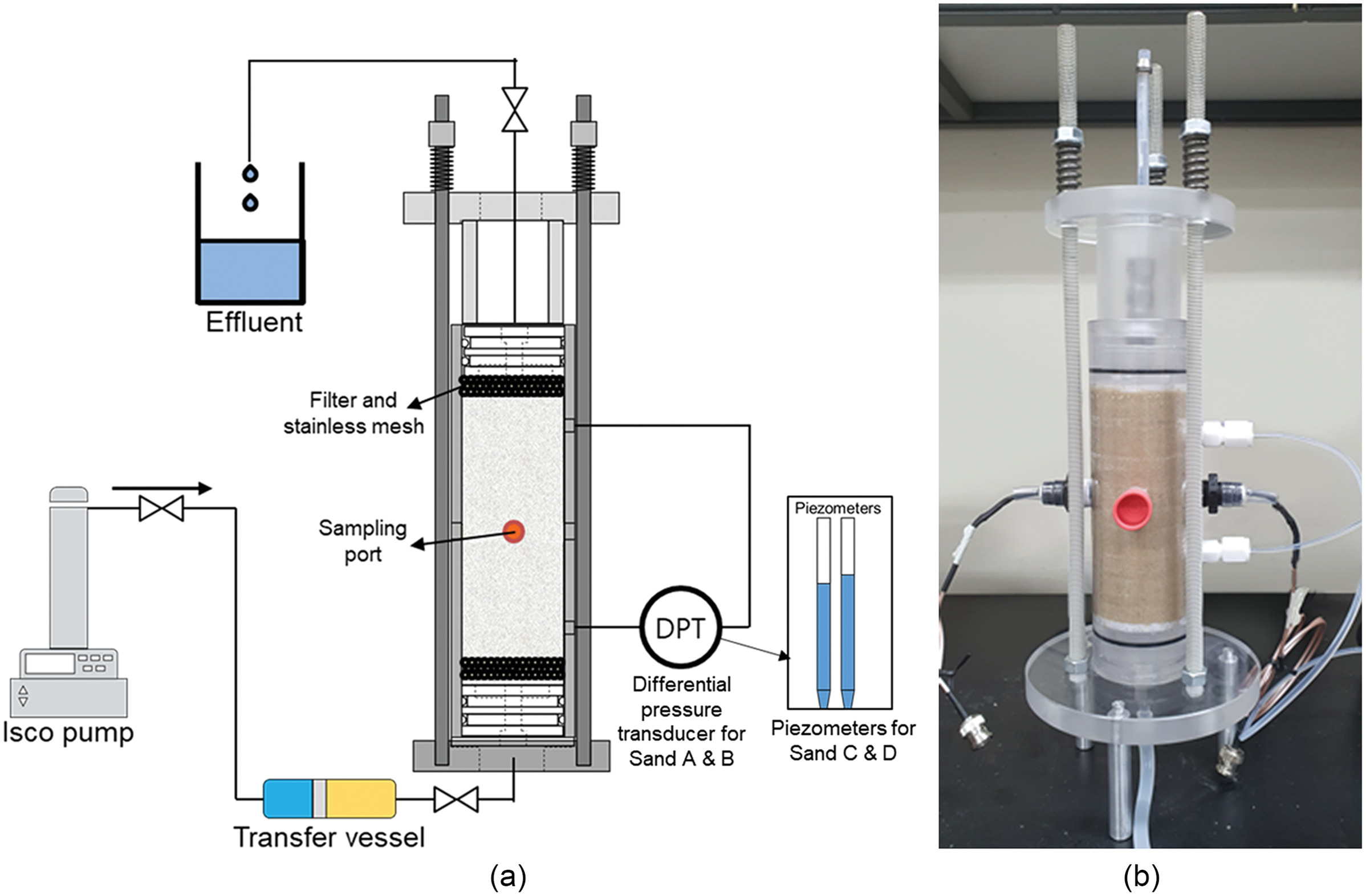
The sand pack column preparation began with the cleaning of the polycarbonate column with ethanol solution (). The other wetting parts, such as fittings and tubing, were autoclaved at 121°C for 15 min. The sand samples were dried in an oven at 120°C for more than one day prior to packing [ASTM D2216-19 (ASTM 2019)]. A dry sand pack column was prepared by hand-tamping one of the four sands listed in Table 1. The initial void ratios of the prepared sand packs ranged from 0.562 to 0.633, which corresponded to a porosity range of 0.360–0.388, as shown in Table 3. The pore volume in the sand column was approximately . The top and bottom of the column contained an aluminum mesh and a layer of glass beads with a diameter of 1.5 mm. In addition, the springs at the top of the column confined the height change by applying a vertical stress of 100–150 kPa. Subsequently, the sand pack column was saturated through several cycles of purging and vacuuming followed by the injection of deionized water (DIW).
| Run symbol | Column experiment runs | |||||||
|---|---|---|---|---|---|---|---|---|
| A-R1 | A-R2 | B-R1 | B-R2 | C-R1 | C-R2 | D-R1 | D-R2 | |
| () | 0.621 (0.383) | 0.597 (0.374) | 0.630 (0.387) | 0.604 (0.377) | 0.633 (0.388) | 0.589 (0.371) | 0.562 (0.360) | 0.623 (0.384) |
| () | 0.423 (0.297) | 0.312 (0.238) | 0.309 (0.236) | 0.334 (0.250) | 0.317 (0.241) | 0.288 (0.224) | 0.481 (0.325) | 0.349 (0.259) |
| 0.87 | 0.93 | 0.66 | 0.77 | 0.75 | 0.84 | 0.93 | 0.72 | |
| (%) | 14.5 | 21.7 | 21.1 | 20.5 | 22.1 | 22.1 | 18.6 | 19.7 |
| (%) | 14.5 | 22.7 | 25.1 | 20.1 | 24.1 | 24.4 | 18.8 | 20.3 |
| (%) | 22.9 | 31.3 | 39.0 | 32.2 | 35.0 | 34.4 | 27.1 | 31.1 |
| () | 0.013 | 0.010 | 0.072 | 0.090 | 0.80 | 0.92 | 4.1 | 1.5 |
| () | 0.0055 | 0.0030 | 0.0013 | 0.025 | 0.13 | 0.34 | 0.42 | 0.51 |
| 0.41 | 0.30 | 0.018 | 0.27 | 0.17 | 0.37 | 0.10 | 0.34 | |
| () | 178.3 | 195.7 | 183.8 | 200.8 | 221.0 | 203.4 | 220.4 | 201.5 |
| () | 1,006 | 1,566 | 971.9 | |||||
Note: = void ratio; = porosity; = initial relative density; = calcite content from the acid washing method; = calcite content calculated from the calcium ion analysis; = pore volume fraction of calcite; = hydraulic conductivity; = shear wave velocity; and R stands for the experimental run. The subscripts and indicate the initial and final value, respectively. The superscript indicates the shear wave velocity measured from free-free resonant column (FFRC) test.
The column experiments were repeated two times for each sand to check the repeatability of the results. Table 3 shows the initial conditions of the prepared columns; a total of eight columns were prepared, two columns for each sand. Each experimental run was named after its sand type (i.e., Sand A, B, C, and D) and the number of repetitions, i.e., A-R1, A-R2, B-R1, and B-R2, where R stands for the experimental run while the following number indicates the number of repetitions. The relative density showed a fairly wide range, from 66% to 93% between sands, due to different gradations. In this study, the duplicates were designed to have similar relative density values and hence consistent initial hydraulic conductivity, , values prior to MICP treatment. For instance, D-R1 and D-R2 had relative densities of 93% and 72%, respectively, owing to slightly different compactive effort, but they showed consistent initial hydraulic conductivity, , values of and , respectively. Likewise, among the duplicates of each sand, the initial hydraulic conductivity values consistently ranged in the same order.
MICP Treatment Program
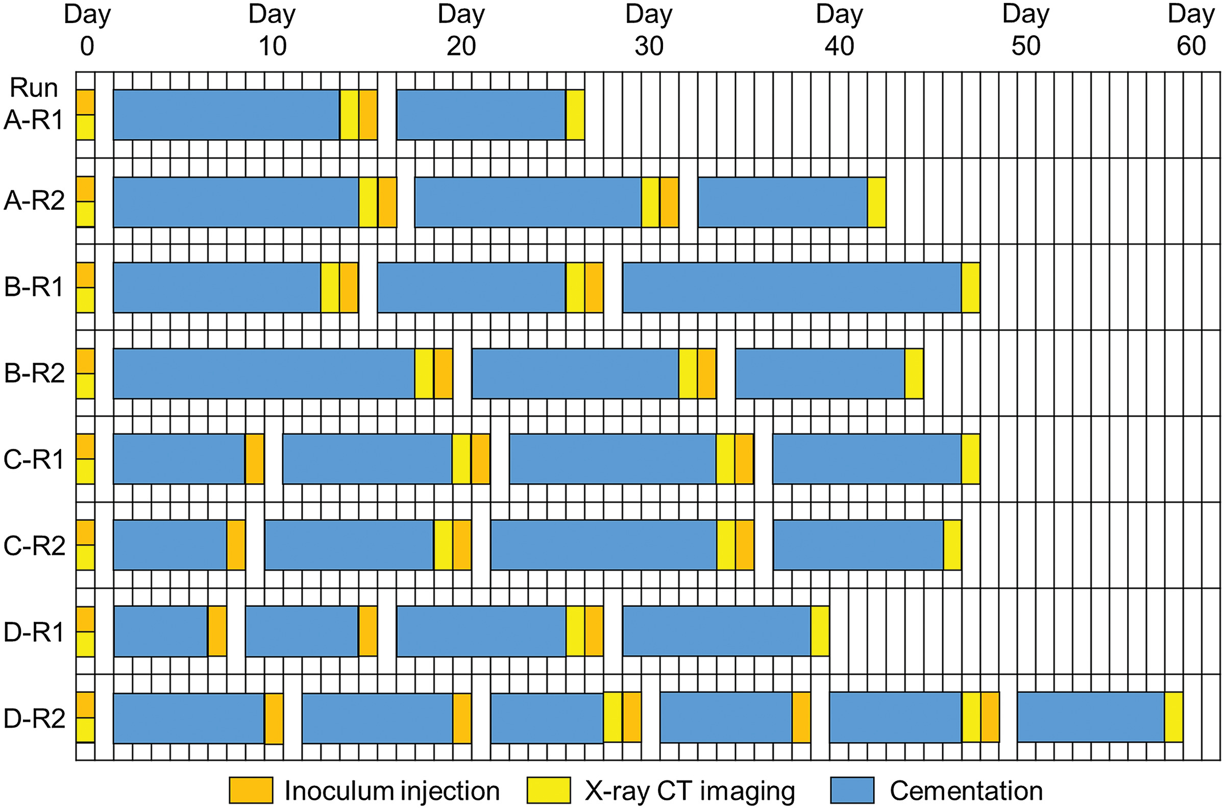
The first treatment phase was the inoculation of the model bacteria (Phase 1), in which three pore volumes of the bacterial solution () were injected at a constant flow rate of . The retention time following inoculation was more than 36 h to allow the inoculated bacteria to attach onto sand grains. In the second treatment phase (Phase 2), three pore volumes of the rinsing solution were injected at a constant flow rate of to facilitate bacterial attachment, and at the same time, to displace residual suspended bacteria in the pore space. Immediately after the second phase, the third phase began with an injection of the cementation solution for three pore volumes at a constant flow rate (Phase 3). The solution injection for three pore volumes () was completed within 30 min. A retention time of more than 20 h was then given to ensure completion of the MICP reaction. The pulsed injection of the cementation solution was repeated every day, which provided a MICP reaction time under no-flow conditions of more than 23 h. The cementation solution injection (Phase 3) was repeated 21–39 times until a CC of achieved. Fig. 3 shows the treatment schedules of all the column tests conducted in this study. Note that the column tests with Sands C and D required additional bioaugmentation treatments in the early stage of treatments due to low reaction rates of urea hydrolysis (see Fig. 3). However, after a moderate level of was achieved, the urea hydrolysis increased to a sufficient level, and only additional cementation solution injections (Phase 3) were repeated.
The solutions were injected at a constant flow rate, and the flow rate differed with the grain size: for Sands A and B, for Sand C, and for Sand D, respectively. The flow rates were determined for two conditions: (a) minimal precipitation during fluid injection, and (b) proper differential pressure measurement for hydraulic conductivity estimation. First, the duration for the cementation solution injection was particularly restricted to be less than 30 min to minimize the MICP reaction occurring during fluid injection and avoid unwanted precipitation close to the fluid inlet. Therefore, the minimum flow rate was set to be to inject 330-mL solutions. Second, the flow rate for each sand was determined by monitoring the compatibility of the differential pressure responses as measured by the differential pressure transducer or the piezometers. As the grain size increases, the hydraulic conductivity increases, and thus the differential pressure for a given flow rate is reduced. Therefore, the highest flow rate was used in Sand D, and the lowest flow rate was used in Sand A. The flow rates used in this study correspond to Reynolds numbers () of , which indicates that the flow velocity regime was laminar. The hydraulic conductivity was calculated based on Darcy’s law and from the differential pressure responses acquired during the solution injections that lasted . Particularly for Sands A and B, the hydraulic conductivities, , of the sand pack columns were additionally measured by the falling-head test method [ASTM D5084-16a (ASTM 2016)]. Comparison between the values from the two methods allowed for verification of measurement consistency and examination of the possible occurrence of clogging in the vicinity of inlet and outlet ports.
Chemical Analyses—Monitoring of Urea Hydrolysis and Content
Pore fluid samples () were collected before and after the cementation solution injection (i.e., Phase 3) through the sampling port at the column. The pore fluid sample was used for the following biochemical analyses after filtering it through a 0.22-μm syringe filter: 1 mL for dissolved calcium ion mass, 1 or 0.1 mL for urea consumption (Knorst et al. 1997), and the remainder for pH. The consumptions of calcium ions and urea imply the ureolytic activity in sand columns. When the urea hydrolysis activity was sufficiently high, the cementation solution injection (Phase 3) was repeated. In contrast, if it was too low, the MICP treatment process was reinitiated with another bioaugmentation injection.
The concentration of the dissolved calcium ion in the aqueous samples was measured using an ICP-OES (Agilent 720 ICP-OES, Agilent, Santa Clara, CA, USA). The change in calcium concentration in the pore fluids not only allowed monitoring of the ureolytic activity of the inoculated bacteria, but also enabled the estimation of the amount of crystals precipitated. Herein, it was assumed that all the consumed calcium ions were converted to solid crystals, mostly calcite, and the solubility of in pore fluids was negligible. Accordingly, gradual increases in the within sand pack columns were quantitatively assessed over the course of the repetitive MICP treatments.
In addition, the urea concentration in the fluid samples was also measured by following the colorimetric urea assay protocol by Knorst et al. (1997). The urea in the fluid was reacted with a urea reagent composed of 50 mL of pure ethanol, 12 mL of hydrochloric acid, and 2 g of p-dimethylaminobenzaldehyde to generate color, which was quantified with the optical density (OD) at a wavelength of 422 nm. The obtained OD value was converted to urea concentration. Monitoring of the urea consumption provided complimentary information to the dissolved calcium ion consumption and was used to ensure the ureolytic activity of the inoculated bacteria.
Upon completion of each experiment, three sand samples of 2–4 g from the top, middle, and bottom sections were taken to measure using the acid washing method (Choi et al. 2017). The measured values were averaged to obtain the values representative of the corresponding sections. In this study, is defined as the ratio of the mass of minerals to the dry mass of sand. The final values of porosity and void ratio were calculated based on the mass of calculated from the acid washing method (Table 3). In addition, X-ray diffraction analysis (XRD) was conducted to determine the mineralogy of the precipitates in the MICP-treated sand samples.
Time-Lapsed Column-Scale X-Ray Computed Tomography (X-Ray CT)
The vertical distribution and uniformity of the calcium carbonate precipitation was accessed by time-lapsed X-ray CT imaging of the sand columns every 8%–9% during MICP treatments. The specification of the X-ray CT facility and the imaging condition can be found in Tables S1 and S2 as Supplemental Materials. X-ray CT imaging produced a stack of horizontal slice images (XY-sliced images), and each XY-sliced image was composed of pixels with a pixel size of 60.3 μm. Each sliced image had a thickness of 50.9 μm; a total of 2,420–2,582 sliced images were obtained per scan, covering the entire height of the sand pack column. Given the relatively large pixel size, these column-scale scanned images allow examination of whether precipitation occurs in a relatively homogeneous manner over the column height or any locally concentrated precipitation occurs. This assists in determining whether the hydraulic conductivity measurement is representative for a given and conducted with no measurement bias. Note that the high energy in the X-ray killed the model bacteria in the column; therefore, MICP treatment was resumed from Phase 1 with the injection of the bacterial solution after each X-ray CT imaging.
Post-Treatment Examination: Pore-Scale X-Ray CMT and SEM Imaging
Upon completion of each experiment, MICP-treated sands of were sampled from the top, middle, and bottom sections of the column and then dried for high-resolution pore-scale X-ray CMT imaging. The X-ray CMT facility was equipped with a nano-focus open X-ray source tube with a focal spot size of 400 nm and a flat panel detector with pixels (Tables S1 and S2 in Supplemental Materials). As a result, each sliced image contained pixels with a pixel size of ; a total of 2,048 sliced images was obtained from each scan. Each slice has a thickness equal to the pixel size. The fine resolution of the scanned images with the micron-sized pixels enables examination of the effect of grain size on pore-scale precipitation habits of minerals. In addition, scanning electron microscopy (SEM) imaging was carried out on the oven-dried sand samples, which were coated twice with osmium or platinum (JSM-IT800 FE-SEM, JEOL Ltd., Tokyo, Japan).
Results
Estimation of Content (CC)
The final values measured from the acid washing tests upon completion of all column experiments are shown in Figs. 4(a and b). When averaging the values for the entire sand column, the average value was 14.5% and 21.7% for A-R1 and A-R2, 21.1% and 20.5% for B-R1 and B-R2, 22.1% and 22.1% for C-R1 and C-R2, and 18.6% and 19.7% for D-R1 and D-R2, respectively, as shown in Table 3. These values were obtained from the acid washing tests. The XRD analysis and SEM images confirmed that the minerals produced by MICP were calcite (see Fig. S1 in Supplemental Materials). Therefore, herein, the terms “ content” and “calcite content” are used interchangeable (but with the same notation, ).
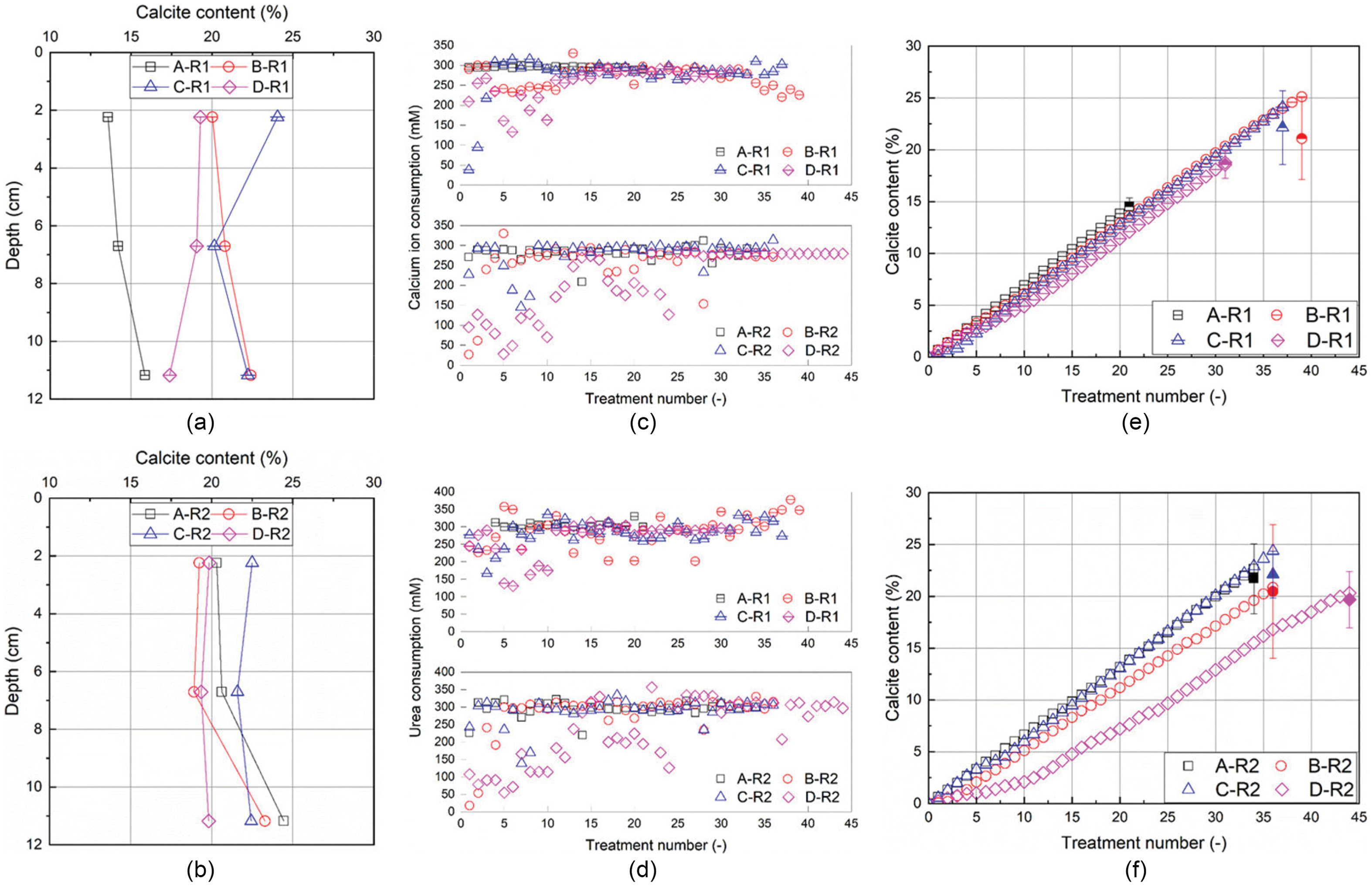
A comparison of the values among the top, middle, and bottom sections shows that the difference in along the vertical direction in each column ranged from 0.2% to 5%. Given the final of more than 20%, it is concluded that minerals precipitated fairly uniformly throughout the columns. Meanwhile, the results in A-R2 and B-R2 particularly show that the of the bottom section was greater than those of the other sections. This indicates possible local blockage given the heavier precipitation at the bottom of the specimen.
The level increased by per injection of 0.3 M cementation solution for three pore volumes in the column experiments with Sands A, B, and C, in which the MICP process consistently consumed more than 90% of urea and calcium treatment without additional bioaugmentation, as shown in Figs. 4(c and d). This implies that the number and activity of attached bacteria was sufficient. In contrast, in the columns with Sand D, the consumptions of urea and calcium ion were less than 70% (or 200 mM consumed out of 300 mM) during the first 10 treatments [Figs. 4(c and d)]. Consequently, the rate in per cementation solution injection was slower than the other sands. However, after 15 treatments the consumption of calcium ions and urea increased to a level greater than 90%, similar to those in the other sands. This indicates that the number of attached bacteria in the columns with Sand D was initially insufficient to hydrolyze 0.3 M urea in pore fluids, primarily because Sand D had the largest grain size, and hence the smallest specific surface area and the least number of contacts per unit volume. This result implies that the grain size has a direct effect on the bacterial attachment and ensuing ureolysis activity in association with the specific surface area and the grain-to-grain contact number.
Figs. 4(e and f) show how changes over the repetitive injections of the cementation solution, which was estimated based on the calcium ion consumption by assuming mass conservation [Fig. 4(c)], and then superimposed with the final values obtained from the acid washing method. As a result, the increased to 14.5% and 22.7% for A-R1 and A-R2, to 25.1% and 20.1% for B-R1 and B-R2, to 24.1% and 24.4% for C-R1 and C-R2, and to 18.8% and 20.3% for D-R1 and D-R2, respectively (Table 3). The estimation based on the calcium consumption appears to overestimate the level compared to the final acid washing results. This is possibly attributable to the combined effects of the calcium conversion efficiency less than 100%, solubility, and flushing out of suspended and weakly attached crystals with fluid injection. Nevertheless, the estimated values from the calcium consumption generally agree well with the acid washing results, showing only a difference of less than 4%. These values estimated using the calcium consumption are used to correlate the hydraulic conductivity with the level in the later sections.
Variations in Hydraulic Conductivity,
The variations in hydraulic conductivity, , during MICP treatments of all the column runs are shown in Fig. 5. The values measured using the differential pressure responses are superimposed with the values measured from the falling-head tests. Table 3 summarizes the results of all the column experiments. The results clearly show that calcite () precipitated by MICP caused a gradual and progressive reduction in in all experiments. In the columns with Sand A (e.g., A-R1 and A-R2) the initial hydraulic conductivities of both runs were . decreased to at the final of 14.5% in A-R1 and to at the final of 21.7% in A-R2. When normalized by the initial hydraulic conductivity, was 0.41 in A-R1 and 0.30 in A-R2, respectively. In column experiments B-R1 and B-R2, the reduction rate was 0.018 at the final of 21.1% and 0.27 at the final of 20.5%, respectively. The column runs with Sand C (i.e., C-R1 and C-R2) show that the reduction rate was 0.17 and 0.37 as the level increased to 22.1% and 22.1%, respectively. In D-R1 and D-R2, was 0.10 at CC of 18.6% and 0.34 at CC of 19.7%, respectively.
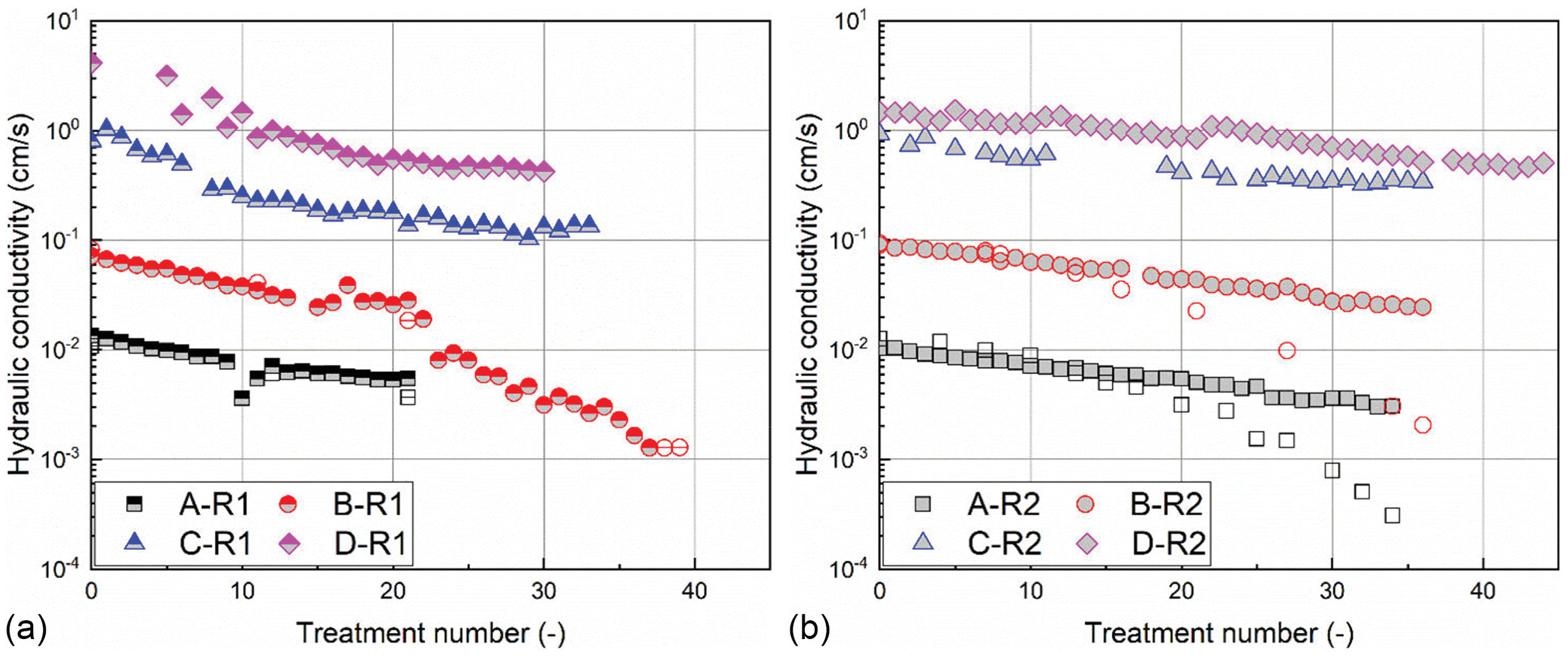
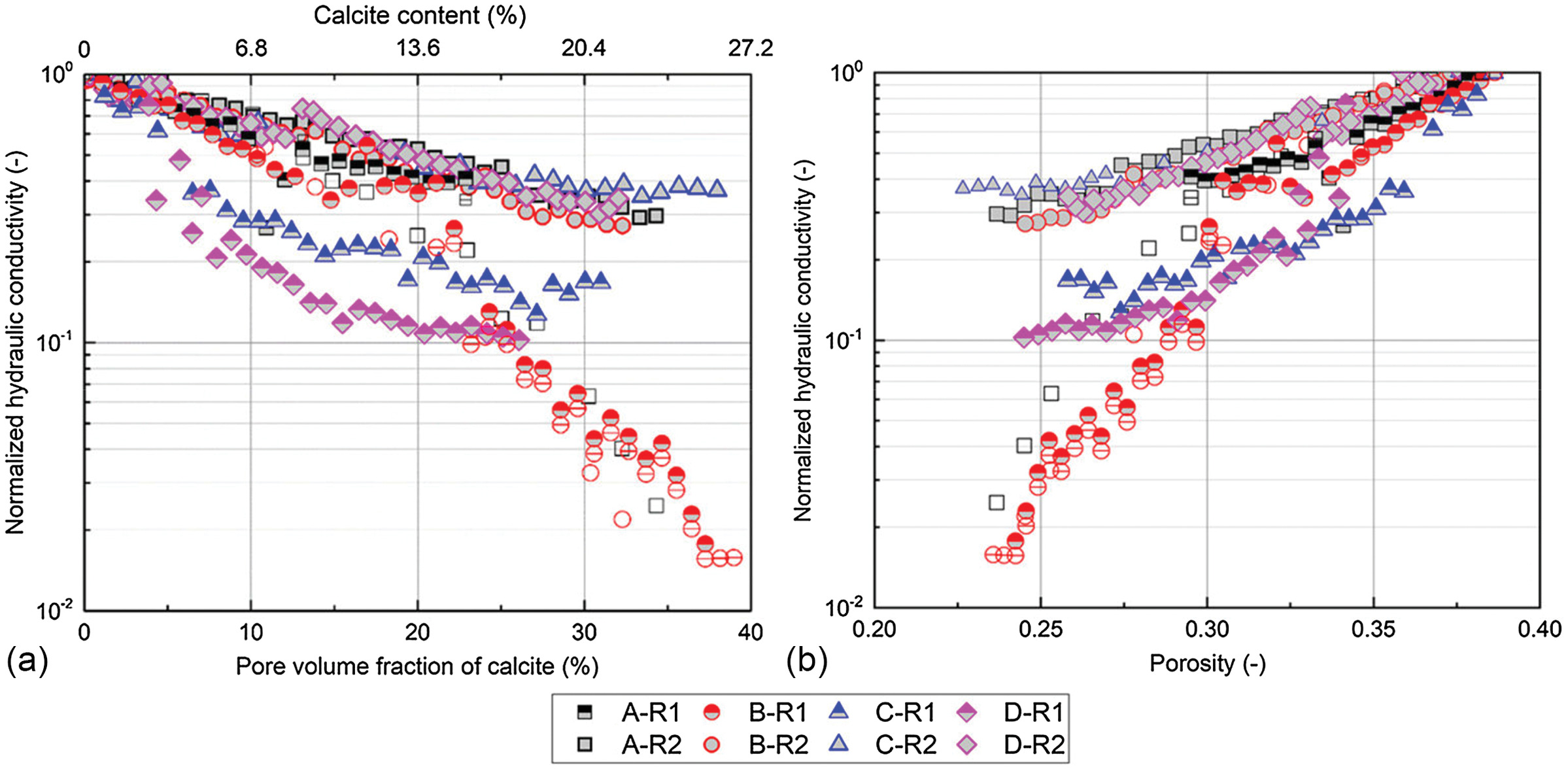
Fig. 6 shows the normalized hydraulic conductivity, , with respect to the pore volume fraction of () or to the porosity, , with precipitation. This result confirms that MICP caused a gradual and consistent reduction in with an increase in or with a decrease in . The reduction was less than one order of magnitude (or by 90%) as increased to 15%, which was equivalent to of 20%, or a porosity reduction from 36%–39% to 30%. The column runs of A-R1, A-R2, B-R2, C-R2, and D-R2 showed remarkably consistent trends. In contrast, B-R1 also showed a gradual reduction until (or ), but thereafter, decreased rapidly, which was possibly due to local clogging. However, this did not occur in B-R2. Further, note that the results of C-R1 and D-R1 showed fairly significant decreases at low and low in the early stage of MICP, but they soon exhibited similar slopes to the other runs in the curves when .
The column experiments with fine sands (Sands A and B) used two approaches for measurement: calculated based on the differential pressure transducer measurement (), which represents the hydraulic conductivity across the middle section, and from the falling-head method, which represents the bulk hydraulic conductivity across the whole column, which can be adversely influenced by clogging in filters, tubes, and fluid ports. Consequently, the difference between the two measurement methods can be an indicator of local clogging outside the middle of the specimen. It appears that the values from both measurements agree well with each other in A-R1 and B-R1, as shown in Fig. 5(a). Whereas the results of A-R2 and B-R2 in Fig. 5(b) show that the values based on the falling-head test decrease rapidly and begin to deviate from those from after 15–20 treatments. This deviation was attributable to the local clogging near the bottom close to the inlet, and it was corroborated by the distributions shown in Fig. 4(b), where the level at the bottom section was higher than that at the top and middle sections. This was also confirmed with the X-ray CT profiles in the later section. The clogging close to the top and bottom boundaries was possibly attributable to the upward flow of the cementation solution in association with a high level of the bacterial activity. Whereas the pressure ports for the measurement were located in the center height of the column, apart from the inlet and outlet, and thereby, estimated from was hardly affected by local clogging that was likely occurring close to the fluid inlet and outlet. On the other hand, the columns with the coarser sand (C and D) appear to have fairly uniform distribution with differences less than 0.5% among the sections, which implies no local clogging. However, the cause of the significant reduction in B-R1, which was also detected by the DPT, is less clear, but may be attributed to clogging in the pressure ports or tubes connected to the differential pressure transducer.
Column-Scale X-Ray CT Imaging Results
Representative column-scale vertically sliced (or XZ-sliced) images of the sand columns from the baseline scan to the final scan with the final from Run 2 is shown in Fig. 7(a). The acquired images demonstrate that the accumulation of minerals increases the density of the sand, which in turn raises X-ray attenuation. The X-ray attenuation is expressed as CT number (or gray-scale value) in an image voxel. Fig. 7(b) shows the change in the CT number (or ΔCT number) with the accumulation of minerals along the sand column length. Herein, a change in the CT number (or ΔCT number) of each sliced image was obtained by subtracting the average CT number of each baseline sliced image from that of the following scans. In addition, the standard deviation (STD) in ΔCT number of each profile was adopted to assess the uniformity in precipitation, as denoted in Fig. 7(b).
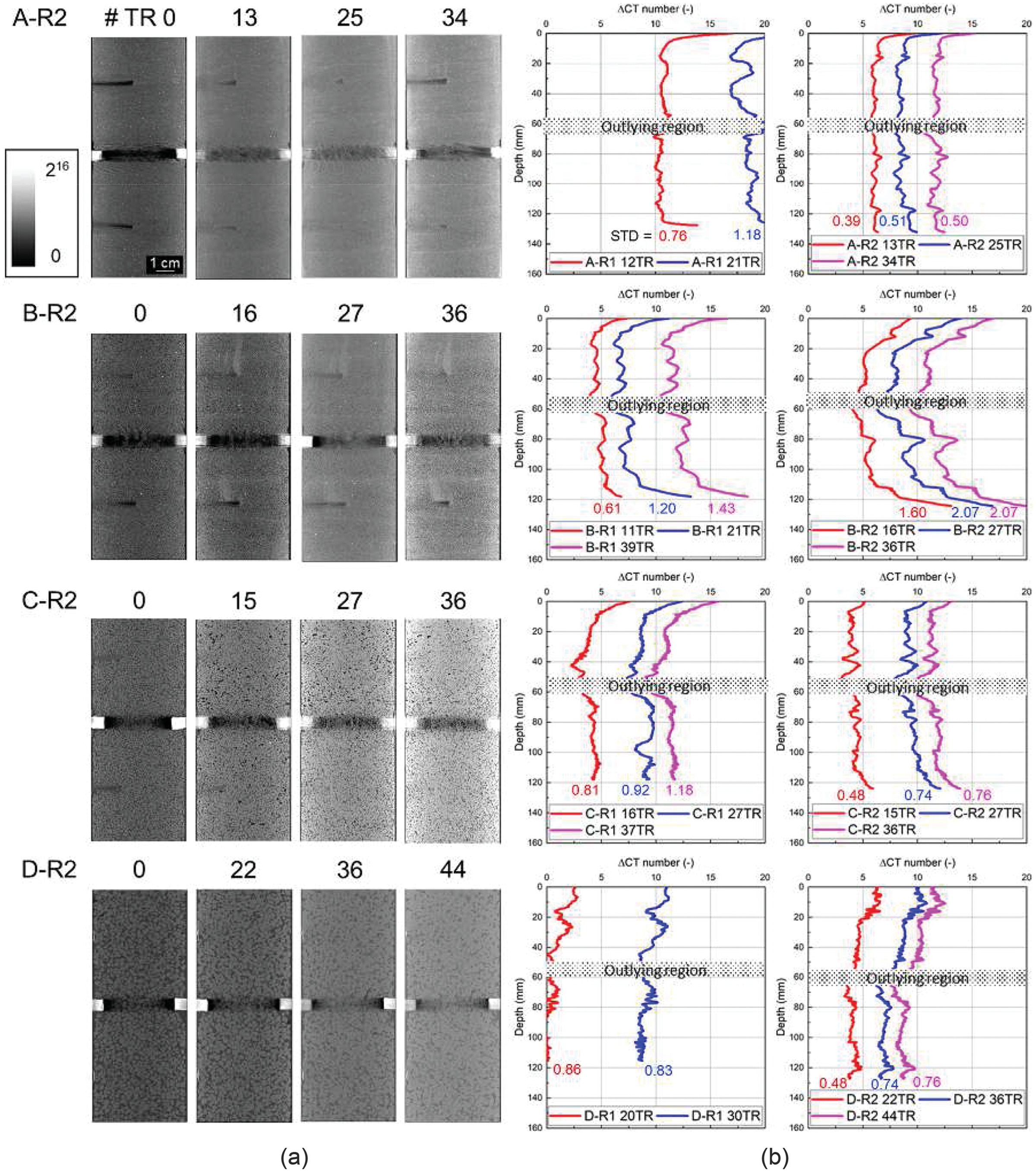
The profiles of Sands A, C, and D show STD values less than 1.2 and a majority less than 0.7–0.8, which supports relatively uniform distributions of minerals. In contrast, the STD values in B-R1 and B-R2 were 1.43 and 2.07 at maximum, respectively, which implies the heterogeneous precipitation in B-R1 and B-R2. Particularly, the abrupt increases in the ΔCT numbers indicating more concentrated precipitation of were observed at the bottom part in B-R1 and at the top and bottom sections in B-R2. This is consistent with the CC results from the acid washing tests shown in Figs. 4(a and b). Meanwhile, the results of C-R1 and D-R1 indicate that more mineral precipitation occurs in the top part of the column. This could be attributed to the early reductions in the initial stage, shown in Fig. 6(a).
Scanning Electron Microscopy (SEM) Imaging Results
SEM images of MICP-treated sands sampled from the sand columns after the experiments are shown in Fig. 8. The SEM images from all columns confirm that the majority of the precipitated minerals had regular cuboidal and rhomboidal shapes, which indicate calcite as the mineralogy of precipitates (van Paassen 2009; Wang et al. 2019b). The use of the treatment solutions with relatively low concentrations of urea and calcium chloride, use of a rinsing solution, and sufficient retention time, promoted calcite mineral formation in this study, which also corroborates the previous observations in van Paassen (2009) and Al Qabany et al. (2012).
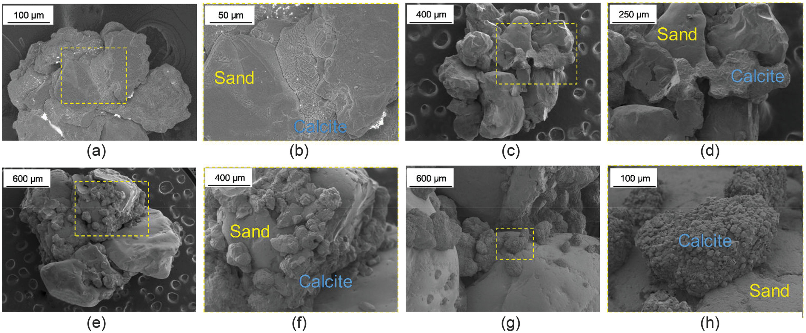
The size of the precipitated mineral aggregates ranged from tens of micrometers to hundreds of micrometers. In the fine sands (Sands A and B), crystals were mostly formed at the grain-to-grain contacts, with minimal calcite precipitation occurring on the exposed grain surfaces. This implies that the bacteria were preferentially concentrated at grain contacts, causing a contact-cementation type of precipitation pattern. On the other hand, in the coarse sands (Sands C and D), minerals were precipitated on both the grain contacts and open grain surfaces. This indicates that the bacteria were more uniformly distributed around the grain surfaces, which consequently produced a grain-coating type of precipitation habit. This is further discussed in the observed precipitation patterns by MICP with the X-ray CMT images in the next section.
Discussion
Pore-Scale Precipitation Habits: Effect of Grain Size
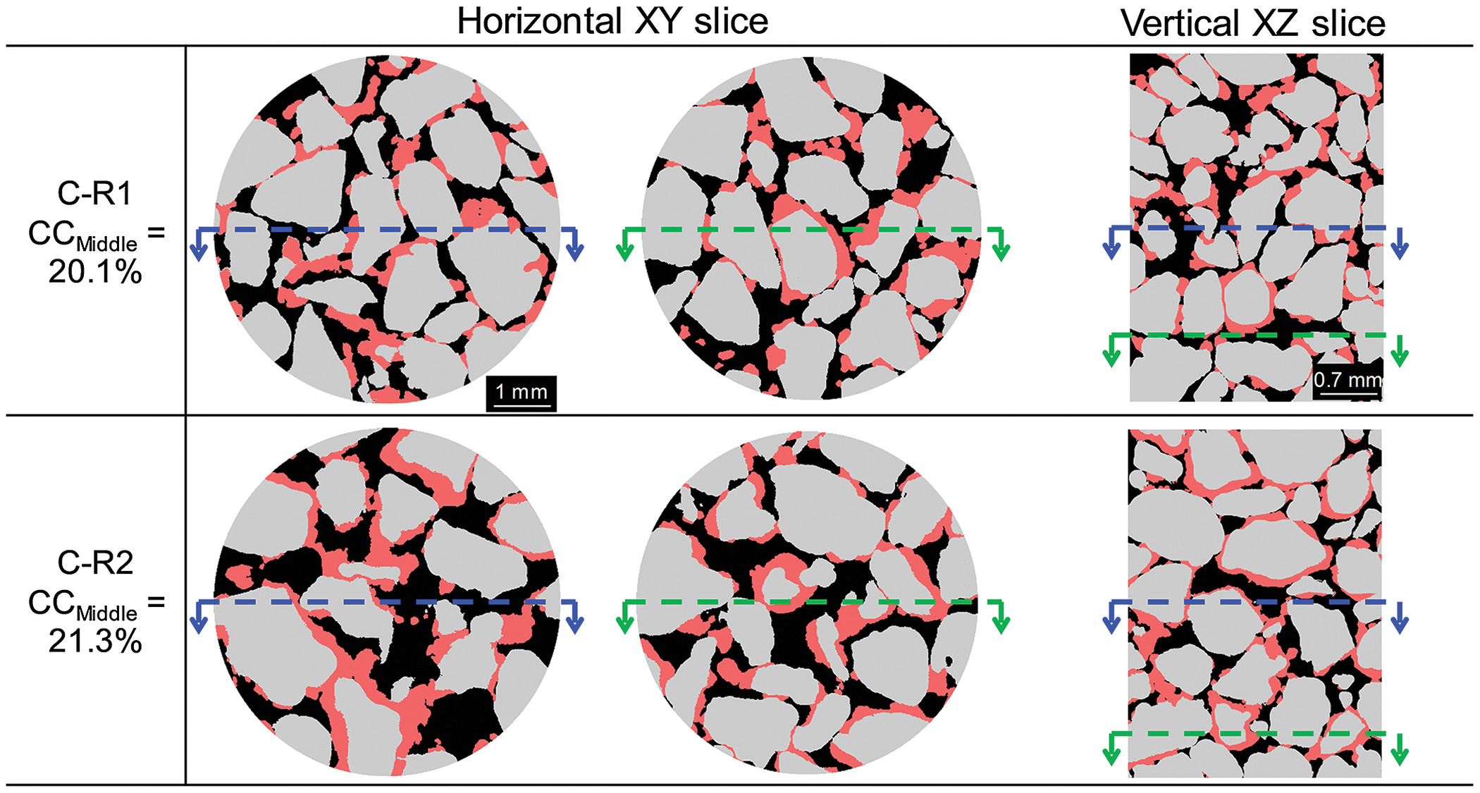
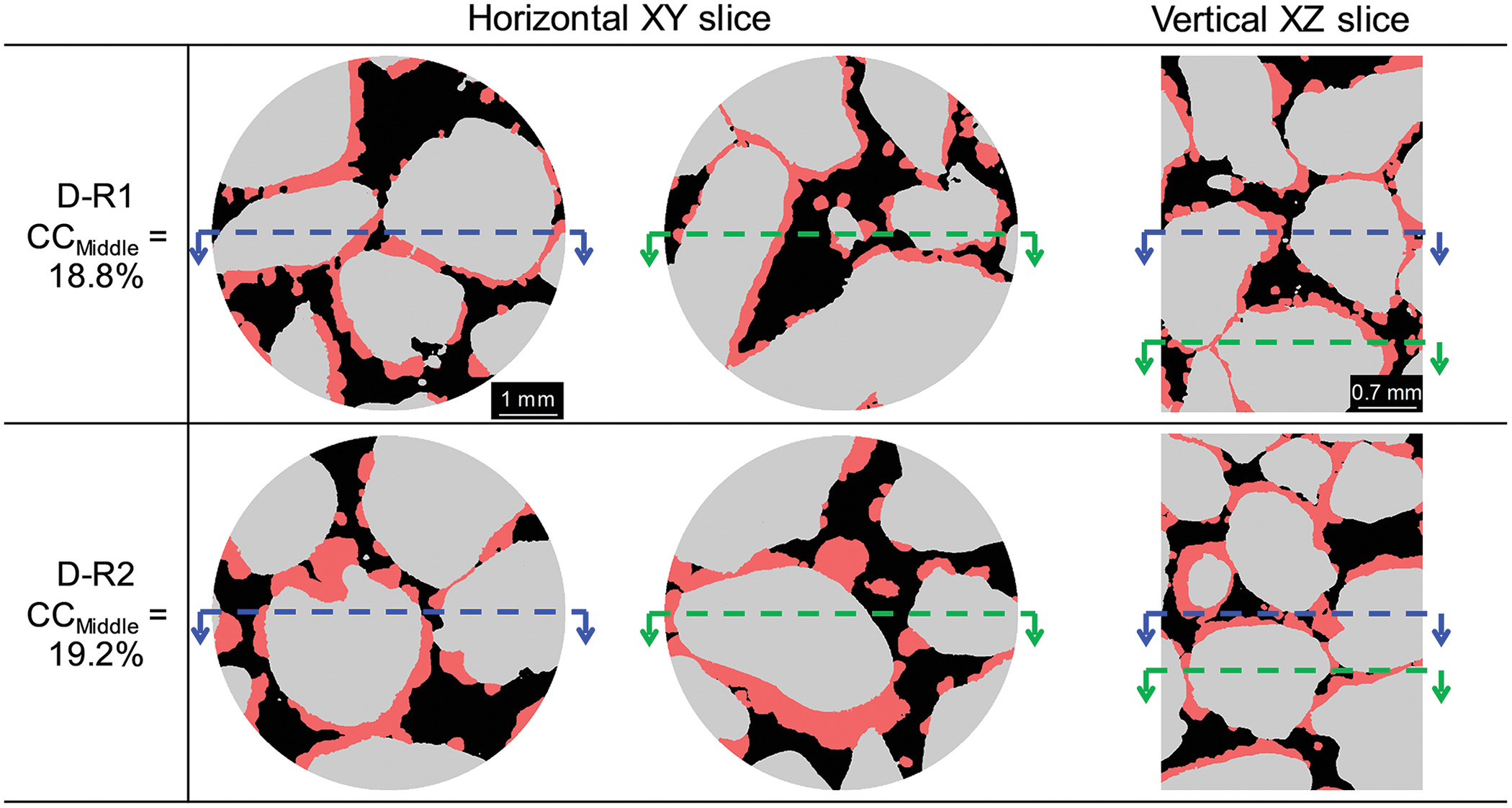
Representative XY- and XZ-sliced images of Sands A–D, taken by using X-ray CMT as the post-treatment examination after the termination of the column experiments, are shown in Figs. 9–12. These high-resolution images capture the pore-scale precipitation patterns in MICP-treated sand with a pixel size range of 4–8 μm. The relevant phases include the solid sand grains, minerals, and pores; and these phases were segmented with the threshold method.
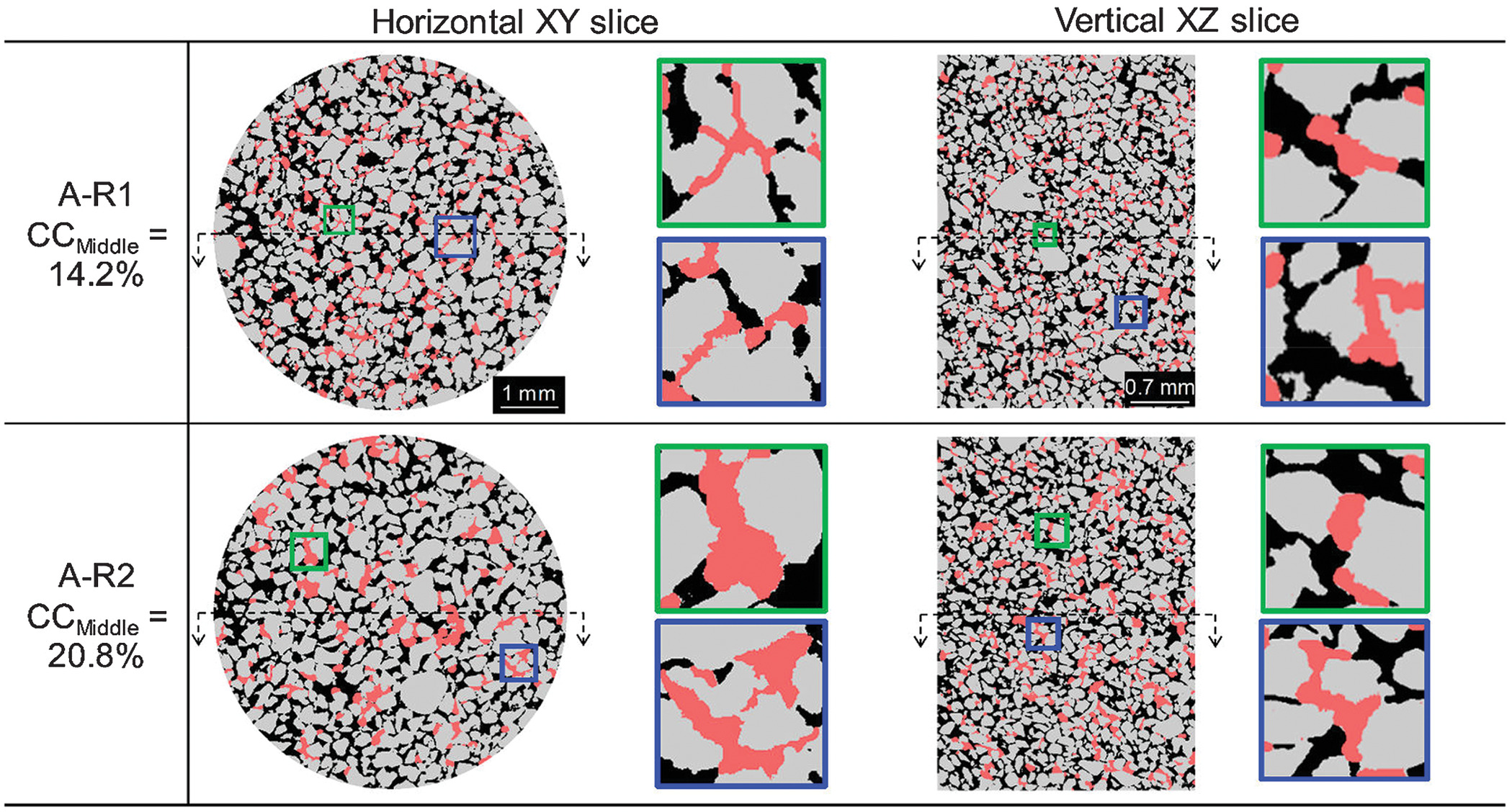
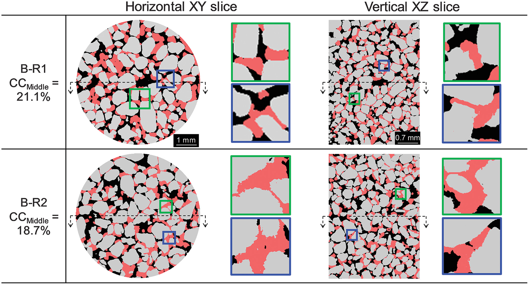
The CMT images of Sands A and B in Figs. 9 and 10 clearly reveal that in fine sands, crystals were primarily precipitated and condensed at the grain contacts, bridging adjacent grains. Moreover, the MICP caused preferential precipitation in small pores and at particle contacts, with less precipitation in large pores or exposed particle surfaces. Despite the levels as high as 15%–24%, a significant portion of the grain surfaces remained free of precipitate. This is consistent with the SEM images shown in Fig. 8, which indicates that the bacteria prefer to be attached at the grain-to-grain contacts and small pores, but it is less likely to be attached to the open grain surfaces exposed to large pores. When the rinsing solution and cementation solution were injected, the fluid flow displaced and flushed the suspended bacteria in pores. In addition, the fluid flow generated shear-induced detachment of the bacteria from particle surfaces. The bacteria attached to the grain surfaces exposed to large pores were more prone to the shear detachment rather than those at grain contacts and in small pores (Stoodley et al. 1999). Therefore, the contact-cementing and grain-bridging habits were predominant in precipitation rather than the grain-coating behavior, because of the preferential attachment to and selective survival in the small pores and grain contacts of bacteria during repetitive pulsed treatment injections.
In contrast, the pore-scale precipitation habit in coarse sands differs from that in fine sands. The X-ray CMT images of Sands C and D in Figs. 11 and 12 reveal that crystals more uniformly coated the grain surfaces. This suggests, in contrast to the aforementioned observations in fine sands, that the bacteria were attached on the grain surfaces in coarse sands, with no particular preferential location of attachment. It can be hypothesized that this distribution type in coarser sands is attributable to the limited number of grain contacts and the limited surface area owing to the large grain size. Bacteria require solid surfaces for their attachment and to thrive on. An increase in grain size leads to decreases in specific surface area and number of grain contacts per bulk volume (or grain contact density). As an example, with an assumption of uniformly sized spherical grains and a void ratio of 0.613 for simplicity, the total surface area of Sands A–D in is 177, 74.4, 28.6, and , respectively. Likewise, the number of grains in is more than 120,000 in Sand A, and decreases to in Sand B, in Sand C, and less than 50 in Sand C, respectively. By assuming an average coordination number of 6, the total number of grain contacts per is more than 700,000 in Soil A, and exponentially decreases to less than 300 in Soil D. Accordingly, those coarse sands (Sands C and D) provide only limited grain contacts and grain surfaces, compared to those in the finer sands (Sands A and B). Therefore, a lesser number of bacterial cells were attached and active for urea hydrolysis and ensuing mineral precipitation, which resulted in the low urea consumptions in the column experiments with Sands C and D (Fig. 8). As mentioned, the low urea consumptions called for the repeated bioaugmentation in the initial stage, which presumably facilitated the attachment of bacteria on the exposed grain surfaces. As a result, the bacteria attached on exposed grain surfaces as well as those at the grain contacts contributed to the mixed precipitation pattern. This is corroborated with the observations from the SEM images shown in Fig. 8. As the total amount of inoculated bacterial cells per soil volume also affects the pore-scale precipitation habit, it is worth noting that MICP treatment with no further bioaugmentation in such coarser sands may have caused a different precipitation pattern, possibly a habit close to the one observed in finer sands.
Comparison of Reduction Data to Previous Literature Data
Most prior studies have measured and reported the hydraulic conductivity of soils before and after MICP treatment as a secondary indicator to confirm calcite precipitation. However, measuring the hydraulic conductivity of MICP-treated soils is often challenging because precipitation can occur anywhere in the wetting part of the test configuration. Particularly, uncontrolled precipitation in a flow path outside the specimen (i.e., test device plumbing) would result in biased measurements. Heterogeneous/preferential precipitation within a specimen can also cause a variation of orders of magnitude. Therefore, comparison of the measured reduction trends with the previously published literature data provides the opportunity to examine the effect of nonuniformity of calcite precipitation and test configuration. Fig. 13 shows the normalized hydraulic conductivity, , with respect to the porosity and the pore volume fraction of calcite. Herein, the hydraulic conductivity results from the previous MICP studies with concentrations of urea and calcium source less than 0.5 M are extracted and plotted together (e.g., Al Qabany and Soga 2013; Martinez et al. 2013; Gomez and DeJong 2017). Typically, the level of calcite content can be divided into three levels: low level as 3%–5%, medium level as 6%–8%, and high level as 10%–12% (DeJong et al. 2022). Field-scale MICP demonstration often aim to achieve a below 10% (van Paassen 2011; Gomez et al. 2014; Ghasemi and Montoya 2022). Therefore, from a practical point of view, the reduction at is examined, which is approximately equivalent to given the general porosity range of poorly graded loose sands. Here, the values measured by the pressure difference, , (with DPT or piezometers) is used, while excluding the results of C-R1 and D-R1 due to the measurement errors that occurred at the first few points.
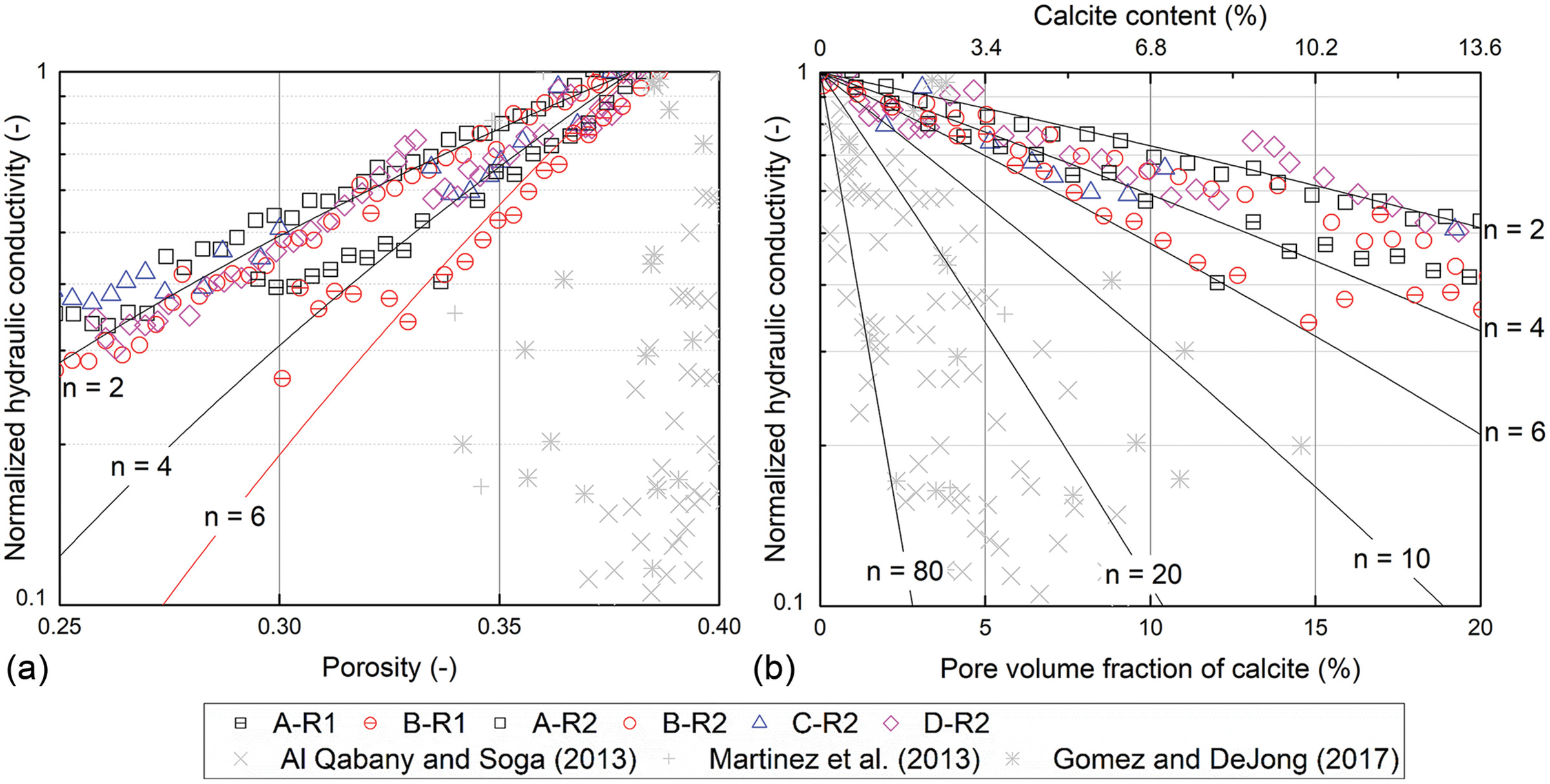
The results show that the reduction trends in literature data are faster than those in this study. For example, in previous studies, a low of 10% will reduce by one order of magnitude or more. It is noted that most previous experimental studies have measured the bulk hydraulic conductivity of sand samples by using the falling-head and constant-head permeability tests or by using the pressure difference across specimens at a constant flow rate. Hence, nonuniform cementation within specimens or local clogging of in the vicinity of the inlet and outlet is likely to have controlled the previously reported data in literature. In contrast, in this study, distribution and column-scale X-ray CT imaging verified near-homogeneous calcite precipitation in the DPT region [Fig. 7(b)], and measurement bias was minimized by measuring the pressure difference across the middle column section. Exceptionally, Dadda et al. (2019) have numerically estimated the values through a Navier–Stokes-based numerical model with X-ray CMT images of some locally sampled sand masses, and the result shows a similar reduction rate. Consequently, the results obtained in this study, in which the cementation is generated in a uniform manner, provide the opportunity to evaluate reductions and calibrate or modify the hydraulic conductivity models, including Kozeny models.
Hydraulic Conductivity Reduction Models for MICP-Treated Sands
Generalized Kozeny–Carman Model
The Kozeny–Carman (KC) model is widely used to capture the effect of porosity reduction on permeability, , and hydraulic conductivity, . A basic formulation of the KC model can be expressed for hydraulic conductivity, , as follows (Carman 1937; Kozeny 1927; Scheidegger 1958):where = absolute permeability; = fluid density; = gravitational acceleration; = fluid viscosity; = shape factor; = porosity; = geometric tortuosity; and = specific surface area per sediment bulk volume. The KC model can be further generalized by substituting the power exponent to and by convoluting the changes in the geometric tortuosity and specific surface area in a single shape factor term. Thereby, the normalized hydraulic conductivity, , can be expressed as a function of the normalized porosity, , as follows:where the subscript indicates the initial untreated baseline condition. The comparison shown in Fig. 13(a) reveals that the generalized KC model can predict the measured reduction trends with an exponent, , of 2–6.
(1)
(2)
Kozeny Grain-Coating Model
A Kozeny grain-coating model is a model derived from the Kozeny model by assuming that the mineral precipitation uniformly coats soil particles (Kleinberg et al. 2003; Noh et al. 2016; Baek et al. 2019). The Kozeny grain-coating model expresses the normalized hydraulic conductivity () as the pore volume fraction of calcite (or calcite pore saturation): . The detailed derivation is described in the Appendix. As shown in Fig. 13(b), the exponent, , contributes to the decrease in hydraulic conductivity, and as increases, the hydraulic conductivity reduction accelerates. The term () is identical to ; therefore, this model is equivalent to the generalized Kozeny–Carman model [Eq. (2)]. Accordingly, the Kozeny grain-coating model with an exponent for also shows good agreement with the measured data in this study. Meanwhile, the Kozeny grain-coating model requires an value of 10–80 to fit the previously published data [Fig. 13(b)].
However, at higher cementation levels, such as , a local blockage becomes more probable, which results in a drastic reduction in hydraulic conductivity [see B-R1 in Fig. 5(a) as an example]. This is consistent with Baek et al. (2019), in which abiotic precipitation of from supersaturated solutions exhibited a uniform grain-coating behavior and a sharp reduction in due to clogging when . In their study, such a clogging-driven reduction rate corresponded to an for the Kozeny grain-coating model while showed a gradual decrease when with (Baek et al. 2019).
Other Hydraulic Conductivity Reduction Models
The additional hydraulic conductivity models, including the Dai–Seol model (Dai and Seol 2014), effective porosity model (Wang and Nackenhorst 2020), and Panda–Lake model (Panda and Lake 1994) can also be evaluated, as shown in Fig. 14. A detailed description of these models can be found in the Appendix.
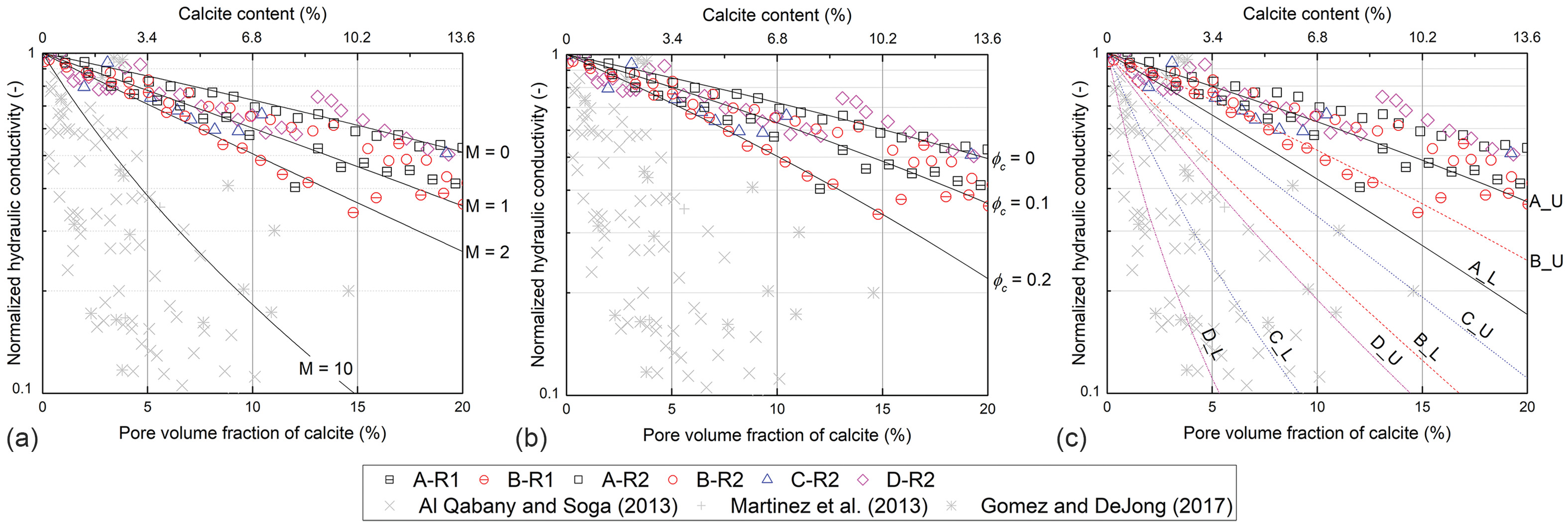
The Dai–Seol model, a derivative of the Kozeny–Carman equation, is based on the statistical results from a number of pore network modeling studies of tortuous flows, in which crystal precipitation is randomly generated (Dai and Seol 2014). The model is defined aswhere = fitting parameter and ranges from 0.1 to 4. With the relationship between the relative porosity and as and Eq. (2), the normalized hydraulic conductivity, , is expressed as a function of pore volume fraction of inclusion material, calcite () in this case, as follows:where = fitting parameter, which ranges from 0.1 to 4, and the variables with subscript denote the values at a given . The relative porosity, , is defined as . Fig. 14(a) shows that the Dai–Seol model with from 0 to 2 predicts the measured reduction trends in this study, which is consistent with the typical range of tortuosity and specific surface area. On the other hand, fitting the model to previously published data requires the value to be greater than 10.
(3)
(4)
The second model is the Kozeny–Carman-based effective porosity model (Wang and Nackenhorst 2020). This model introduces the concept of the effective porosity, , defined as the volume fraction of pore that is still connected to each other after calcite precipitation, and the critical porosity, , defined as the porosity at which the permeability becomes zero. Koponen et al. (1997) expressed the effective porosity, as follows:where is a constant; is defined as ; and is the total porosity. The characteristics of pore structures determine and . Considering the effective porosity in the modified Kozeny–Carman model, Eq. (1) becomeswhere the subscript indicates the initial value. Fig. 14(b) shows the predicted reductions while varying the critical porosity . The critical porosity controls the rate of reduction for a given porosity reduction; the higher indicates a faster rate of reduction. The measured mostly falls into the bounded region with and 0.2. Meanwhile, fitting of the effective porosity model to previously published data requires , which seems not physically plausible in soils.
(5)
(6)
Finally, the Panda–Lake model (Panda and Lake 1994), which is also a derivative of the Kozeny–Carman model, introduces three reduction factors associated with mineral precipitation: porosity reduction factor (), tortuosity reduction factor (), and specific surface area reduction factor (). These three factors are determined based on the morphological characteristics of calcite precipitate distribution, including pore-lining, pore-filling, and pore-bridging behavior, respectively. The most relevant model to the observed pore-scale MICP pattern is the pore-lining behavior. Among the three factors, is assumed to be 1, owing to its minimal effect on pore structure (Panda and Lake 1994). Therefore, the Panda–Lake equation can be rewritten as follows:where the subscript indicates the initial value; is the specific surface area of host soil; and is the specific surface area of minerals. As the host particle size decreases and the specific surface area of the particle increases, the rate of reduction becomes faster. And, as the size of precipitates decreases and the specific surface area of increases, the rate of reduction becomes faster. can be calculated assuming a spherical particle with a mean grain size. Therefore, the important and tunable variable is only the specific surface area of minerals, , in this model. The lower and upper limits of were estimated based on SEM images, assuming a spherical crystal sized as 50 and 200 μm. As a result, there are two bounding reduction curves for each soil, as shown in Fig. 14(c). The Panda–Lake model predicts a wide variation in reduction trends with the host grain size; however, it appears that the modeling results do not match well with the experimental results of this study.
(7)
Implications to Precipitation Pattern and Hydraulic Conductivity Reduction
The MICP-based soil improvement method is being explored for a variety of geotechnical engineering applications, including (1) soil stabilization and settlement reduction (Choi et al. 2017; van Paassen 2009; Zhao et al. 2014), (2) erosion control (Jiang and Soga 2017; Maleki et al. 2016; Salifu et al. 2016), and (3) liquefaction mitigation (Burbank et al. 2013; Feng and Montoya 2017; Han et al. 2016; Montoya et al. 2013). These MICP-based mechanical improvement practices typically target a moderate cementation level with a from 5% to 10% (e.g., ). If the MICP application up to 10% induces homogeneous and contact-cementing calcite precipitation in sands, the results herein indicate that the hydraulic conductivity reduction would not be substantial. A level of 5%–10% would approximately decrease the porosity by 15% and the void ratio by 20%; such a reduction is expected to reduce by , less than one order of magnitude. The Kozeny–Carman model and the Kozeny grain-coating model with a power exponent of 2–6 could be used to predict the reductions in hydraulic conductivity. It is noted, of course, that the pore-scale precipitation is subject to the precipitation uniformity and the physiochemical characteristics of host soils (e.g., van Paassen 2009; Al Qabany et al. 2012; Al Qabany and Soga 2013; Zhao et al. 2014; Choi et al. 2020; Kim et al. 2020), all of which can cause or contribute to more rapid reduction in the hydraulic conductivity.
The column experiments in this study used a relatively low-concentration cementation solution (300 mM urea and calcium chloride) and rinsing solution and provided sufficient retention time for reaction completion. This provides conditions more favorable for precipitation of calcite, a stable form of minerals, and homogeneously distributed calcite precipitation. For fine sands (Sands A and B), the calcite precipitation is concentrated at the grain contacts, which results in significant increases in stiffness and strength while only reducing the hydraulic conductivity by one order of magnitude. This suggests that the adopted MICP treatment strategy would be the most effective in the grain size range from 100 to 600 μm, especially for mechanical reinforcement purposes, such as soil stiffness improvement and erosion mitigation. In coarser soil deposits (), higher cementation levels may be necessary to sufficiently improve the mechanical response.
Conclusions
This study explored hydraulic conductivity reductions in sands caused by MICP and examined the hydraulic conductivity reduction models for MICP-treated sands. In column experiments with different sizes of poorly graded sands, the hydraulic conductivity reduction, change in calcite content, spatial distribution of precipitated , and pore-scale precipitation pattern were examined while attempting to produce homogeneous precipitations over the sand pack columns. The main findings are as follows:
•
The MICP treatment using a rinsing solution and a relatively low-concentration cementation solution (0.3 M) caused gradual yet constrained reductions in of 50%–90%, less than one order of magnitude, until reaching or , which contrasts with previous literature data. While the falling-head test was easily affected by locally concentrated precipitation close to the fluid inlet or outlet, estimation based on measurement across the middle height section of the sand column appeared more reliable.
•
Both the high-resolution X-ray CMT and SEM images revealed the contact-cementing precipitation pattern in fine sands and the mixed habit of contact-cementing and surface-coating precipitation in coarse sands, mainly attributable to the locations of attached bacteria.
•
The results of urea and calcium ion consumptions clearly indicated that fewer bacterial cells were attached and actively involved in urea hydrolysis due to the limited grain contacts and surfaces provided by coarser sands, in comparison to finer sands.
•
Kozeny–Carman type models, particularly the Kozeny grain-coating model and generalized Kozeny–Carman model with a power exponent, , of 2–6, well described the hydraulic conductivity reduction behavior caused by MICP as a function of for the tested range of 0%–20% ( of 0%–13.5%).
This study presents high-quality pore-scale images that contribute to our understanding of the calcite precipitation habits at the pore scale in sands. Additionally, it provides unique hydraulic conductivity data that can be used to develop hydraulic conductivity models for MICP-treated sands. Moreover, the experimental data presented in this study are expected to be particularly valuable if a field-scale MICP strategy seeks to employ a contact-cementing calcite precipitation habit for mechanical reinforcement.
Supplemental Materials
File (supplemental_materials_jggefk.gteng-11570_baek.pdf)
- Download
- 218.83 KB
Appendix. Permeability Reduction Models
Four permeability reduction models due to an inclusion material, herein, calcite mineral, are presented herein. The permeability, , normalized by its initial permeability, , is expressed as the normalized permeability, . As the permeability is directly related to the hydraulic conductivity, note that the normalized permeability, , is identical to the normalized hydraulic conductivity, .
Kozeny Grain-Coating Model
When calcite coats the capillary walls uniformly, the radius of the water-filled pore space is assumed to reduce to . Then, the flow rate through a unit cross-sectional area containing a bundle of parallel cylindrical capillary tubes having an inner radius, , and length, , becomeswhere = number of capillary tubes per unit cross-sectional area; = dynamic viscosity; and = differential pressure. Because the number of capillaries per unit cross section is where is porosity, the permeability is reduced to is related to the initial radius and the reduced radius as
(8)
(9)
(10)
Because of their simplicity, Kozeny-type permeability equations are extensively used, in which the ratio of pore surface area to pore volume is addressed aswhere = shape factor; and = tortuosity. The tortuosity iswhere denotes the flow path length, which is longer than the straight-line distance, , associated with the pressure drop, . The tortuosity, , is related to the electrical formation factor, , and the porosity, , as follows (Hearst et al. 2000):
(11)
(12)
(13)
The above derivation is based on the permeability model for hydrate-containing sediment. Despite the differences between the hydrate and the calcite, the relationship developed for a hydrate-containing grain pack is used in this case because hydrates and calcite are both insoluble and the precipitation patterns are similar. The formation factor in a calcite-saturated medium and the formation factor in a totally water-saturated rock, , are related aswhere is the Archie saturation exponent. Since the pore water volume ratio , Eq. (14) becomes
(15)
(16)
As the grain surfaces are coated with the calcite, the surface area of the water-filled pore volume reduces with increasing . Using the cylindrical pore model, the pore radius without calcite is and the reduced pore radius with calcite is . The surface area ratio is then calculated asand recalling Eq. (10)
(17)
(18)
Thus, Eq. (16) becomes
(19)
Dai and Seol Model
Another extensively used Kozeny-type permeability model is the Kozeny–Carman equationwhere = constant; and is the specific surface of the soil structure. Dai and Seol (2014) developed a Kozeny–Carman-based permeability model that integrated the pore network modeling studies on the tortuosity and specific surface area, , as a function of calcite saturation, . Even though this model was originally developed for hydrate sediments, it was employed due to the similarities of hydrate and calcite. As a result, the overall trend is captured with a range of fitting parameter of 0.1–4:where =relative value. Additionally, the relative porosity of sediment, , changes with , and can be expressed as . Integrating this relationship and Eq. (21) into the Kozeny–Carman equation [Eq. (20)], it becomes
(20)
(21)
(22)
Effective Porosity Model
It is difficult to capture the influence of the modification of pore structure (., pore clogging) on permeability reduction using the basic Kozeny–Carman model. To solve this problem, the concept of effective porosity can be adopted. The effective porosity is a subset of total porosity that represents the volume fraction of pore space that remains interconnected following calcite precipitation (Wang and Nackenhorst 2020; Koponen et al. 1997), which is expressed aswhere = total porosity; = constant; and = critical porosity below which the permeability is equal to zero. With this concept, the Kozeny–Carman model can be modified aswhere = mean particle size of the host grain. Hence, the normalized permeability is expressed aswhere notation denotes the initial values.
(23)
(24)
(25)
(26)
Panda–Lake Model
The Panda–Lake model is also derived from the general Kozeny–Carman model integrating cementation pattern into the model. The equation develops from one form of the Kozeny–Carman modelwhere = shape factor. Panda and Lake (1994) modified this model considering the particle size distribution. Particularly and the are calculated from the statistical parameters of the particle size distribution as follows:where = standard deviation of the particle size distribution; = statistical mean particle diameter of the particle size distribution; and = statistical skewness of the particle size distribution. This model also considers three different cementation pattern of calcite such as pore-lining, pore-filling, and pore-bridging, by incorporating three reduction factors into the model aswhere = porosity reduction factor; = tortuosity reduction factor; and = specific surface area reduction factor. The definitions of each factor areandwhere is a constant ranging between 1 (for thick particles) and 10 (for thin and long crystals); is the ratio of volume to the total solid volume; and is the specific surface area of the crystals.
(27)
(28)
(29)
(30)
(31)
(32)
(33)
(34)
Data Availability Statement
All data, models, or codes that support the findings of this study are available from the corresponding author upon reasonable request.
Acknowledgments
This research was supported by the National Research Foundation of Korea (NRF) grant funded by the Korea government (MSIT) (No. NRF-2022R1A4A5031447). Additional support was provided by the Engineering Research Center Program of the National Science Foundation under NSF Cooperative Agreement No. EEC-1449501. Any opinions, findings, and conclusions or recommendations expressed in this manuscript are those of the authors and do not necessarily reflect the views of the National Science Foundation
References
Al Qabany, A., and K. Soga. 2013. “Effect of chemical treatment used in MICP on engineering properties of cemented soils.” Géotechnique. 63 (4): 331–339. https://doi.org/10.1680/geot.SIP13.P.022.
Al Qabany, A., K. Soga, and C. Santamarina. 2012. “Factors affecting efficiency of microbially induced calcite precipitation.” J. Geotech. Geoenviron. Eng. 138 (8): 992–1001. https://doi.org/10.1061/(ASCE)GT.1943-5606.0000666.
Armstrong, R., and J. Ajo-Franklin. 2011. “Investigating biomineralization using synchrotron based X-ray computed microtomography.” Geophys. Res. Lett. 38 (8): L08406. https://doi.org/10.1029/2011GL046916.
ASTM. 2016. Standard test methods for measurement of hydraulic conductivity of saturated porous materials using a flexible wall permeameter. ASTM D5084-16a. West Conshohocken, PA: ASTM.
ASTM. 2019. Standard test methods for laboratory determination of water (moisture) content of soil and rock by mass. ASTM D2216-19. West Conshohocken, PA: ASTM.
Baek, S. H., J. W. Hong, K. Y. Kim, S. Yeom, and T. H. Kwon. 2019. “X-ray computed microtomography imaging of abiotic carbonate precipitation in porous media from a supersaturated solution: Insights into effect of mineral trapping on permeability.” Water Resour. Res. 55 (5): 3835–3855. https://doi.org/10.1029/2018WR023578.
Burbank, M., T. Weaver, R. Lewis, T. Williams, B. Williams, and R. Crawford. 2013. “Geotechnical tests of sands following bioinduced calcite precipitation catalyzed by indigenous bacteria.” J. Geotech. Geoenviron. Eng. 139 (6): 928–936. https://doi.org/10.1061/(ASCE)GT.1943-5606.0000781.
Carman, P. C. 1937. “Fluid flow through granular beds.” Trans. Inst. Chem. Eng. 15 (1): 150–166.
Chae, S. H., H. Chung, and K. Nam. 2021. “Evaluation of microbially Induced calcite precipitation (MICP) methods on different soil types for wind erosion control.” Environ. Eng. Res. 26 (1): 190507. https://doi.org/10.4491/eer.2019.507.
Cheng, L., R. Cord-Ruwisch, and M. A. Shahin. 2013. “Cementation of sand soil by microbially induced calcite precipitation at various degrees of saturation.” Can. Geotech. J. 50 (1): 81–90. https://doi.org/10.1139/cgj-2012-0023.
Choi, S. G., I. Chang, M. Lee, J. H. Lee, J. T. Han, and T. H. Kwon. 2020. “Review on geotechnical engineering properties of sands treated by microbially induced calcium carbonate precipitation (MICP) and biopolymers.” Constr. Build. Mater. 246 (Jun): 118415. https://doi.org/10.1016/j.conbuildmat.2020.118415.
Choi, S. G., J. Chu, R. C. Brown, K. Wang, and Z. Wen. 2017. “Sustainable biocement production via microbially induced calcium carbonate precipitation: Use of limestone and acetic acid derived from pyrolysis of lignocellulosic biomass.” ACS Sustainable Chem. Eng. 5 (6): 5183–5190. https://doi.org/10.1021/acssuschemeng.7b00521.
Dadda, A., C. Geindreau, F. Emeriault, S. Rolland du Roscoat, A. Esnault Filet, and A. Garandet. 2019. “Characterization of contact properties in biocemented sand using 3D X-ray micro-tomography.” Acta Geotech. 14 (3): 597–613. https://doi.org/10.1007/s11440-018-0744-4.
Dai, S., and Y. Seol. 2014. “Water permeability in hydrate-bearing sediments: A pore-scale study.” Geophys. Res. Lett. 41 (12): 4176–4184. https://doi.org/10.1002/2014GL060535.
DeJong, J. T., et al. 2014. “Biogeochemical processes and geotechnical applications: Progress, opportunities and challenges.” Géotechnique. 63 (4): 287–301. https://doi.org/10.1680/geot.SIP13.P.017.
DeJong, J. T., M. B. Fritzges, and K. Nüsslein. 2006. “Microbially induced cementation to control sand response to undrained shear.” J. Geotech. Geoenviron. Eng. 132 (11): 1381–1392. https://doi.org/10.1061/(ASCE)1090-0241(2006)132:11(1381).
DeJong, J. T., M. G. Gomez, A. C. San Pablo, C. M. R. Graddy, D. C. Nelson, M. Lee, K. Ziotopoulou, M. El Kortbawi, B. Montoya, and T. H. Kwon. 2022. “State of the art: MICP soil improvement and its application to liquefaction hazard mitigation.” In Proc., 20th Int. Conf. on Soil Mechanics and Geotechnical Engineering, 105. London: International Society for Soil Mechanics and Geotechnical Engineering.
De Muynck, W., D. Debrouwer, N. De Belie, and W. Verstraete. 2008. “Bacterial carbonate precipitation improves the durability of cementitious materials.” Cem. Concr. Res. 38 (7): 1005–1014. https://doi.org/10.1016/j.cemconres.2008.03.005.
Feng, K., and B. M. Montoya. 2017. “Quantifying level of microbial-induced cementation for cyclically loaded sand.” J. Geotech. Geoenviron. Eng. 143 (6): 06017005. https://doi.org/10.1061/(ASCE)GT.1943-5606.0001682.
Ghasemi, P., and B. M. Montoya. 2022. “Field implementation of microbially induced calcium carbonate precipitation for surface erosion reduction of a coastal plain sandy slope.” J. Geotech. Geoenviron. Eng. 148 (9): 04022071. https://doi.org/10.1061/(ASCE)GT.1943-5606.0002836.
Gomez, M. G., and J. T. DeJong. 2017. “Engineering properties of biocementation improved sandy soils.” In Proc., Grouting 2017 Technical Papers, 23–33. Reston, VA: ASCE.
Gomez, M. G., C. M. R. Graddy, J. T. DeJong, and D. C. Nelson. 2019. “Biogeochemical changes during bio-cementation mediated by stimulated and augmented ureolytic microorganisms.” Sci. Rep. 9 (1): 1–15. https://doi.org/10.1038/s41598-019-47973-0.
Gomez, M. G., B. C. Martinez, J. T. DeJong, C. E. Hunt, L. A. deVlaming, D. W. Major, and S. M. Dworatzek. 2014. “Field-scale bio-cementation tests to improve sands.” Proc. Inst. Civ. Eng.K Ground Improv. 168 (3): 206–216. https://doi.org/10.1680/grim.13.00052.
Hammes, F., and W. Verstraete. 2002. “Key roles of pH and calcium metabolism in microbial carbonate precipitation.” Rev. Environ. Sci. Biotechnol. 1 (1): 3–7. https://doi.org/10.1023/A:1015135629155.
Han, Z., X. Cheng, and M. Qiang. 2016. “An experimental study on dynamic response for MICP strengthening liquefiable sands.” Earthquake Eng. Eng. Vibr. 15 (4): 673–679. https://doi.org/10.1007/s11803-016-0357-6.
Hataf, N., and A. Baharifard. 2020. “Reducing soil permeability using microbial induced carbonate precipitation (MICP) method: A case study of Shiraz landfill soil.” Geomicrobiol. J. 37 (2): 147–158. https://doi.org/10.1080/01490451.2019.1678703.
Hearst, J. R., P. H. Nelson, and F. L. Paillett. 2000. Well logging for physical properties: A handbook for geophysicists, geologists, and engineers. 2nd ed., 492. New York: Wiley.
Jiang, N. J., and K. Soga. 2017. “The applicability of microbially induced calcite precipitation (MICP) for internal erosion control in gravel-sand mixtures.” Géotechnique 67 (1): 42–55. https://doi.org/10.1680/jgeot.15.P.182.
Jiang, N. J., and K. Soga. 2019. “Erosional behavior of gravel-sand mixtures stabilized by microbially induced calcite precipitation (MICP).” Soils Found. 59 (3): 699–709. https://doi.org/10.1016/j.sandf.2019.02.003.
Jiang, N. J., K. Soga, and M. Kuo. 2017. “Microbially induced carbonate precipitation for seepage-induced internal erosion control in sand-clay mixtures.” J. Geotech. Geoenviron. Eng. 143 (3): 04016100. https://doi.org/10.1061/(ASCE)GT.1943-5606.0001559.
Kim, D. H., N. Mahabadi, J. Jang, and L. A. van Paassen. 2020. “Assessing the kinetics and pore-scale characteristics of biological calcium carbonate precipitation in porous medium using a microfluidic chip experiment.” Water Resour. Res. 56 (2): e2019WR025420. https://doi.org/10.1029/2019WR025420.
Kim, D. S., G. C. Kweon, and K. H. Lee. 1997. “Alternative method of determining resilient modulus of compacted subgrade soils using free-free resonant column test.” Transp. Res. Rec. 1577 (1): 62–69. https://doi.org/10.3141/1577-08.
Kim, H. K., S. J. Park, J. I. Han, and H. K. Lee. 2013. “Microbially mediated calcium carbonate precipitation on normal and lightweight concrete.” Constr. Build. Mater. 38 (Jan): 1073–1082. https://doi.org/10.1016/j.conbuildmat.2012.07.040.
Kleinberg, R. L., C. Flaum, D. D. Griffin, P. G. Brewer, G. E. Malby, E. T. Peltzer, and J. P. Yesinowski. 2003. “Deep sea NMR: Methane hydrate growth habit in porous media and its relationship to hydraulic permeability, deposit accumulation, and submarine slope stability.” J. Geophys. Res.: Solid Earth 108 (B10): 2508–2524. https://doi.org/10.1029/2003JB002389.
Knorst, M. T., R. Neubert, and W. Wohlrab. 1997. “Analytical methods for measuring urea in pharmaceutical formulations.” J. Pharm. Biomed. Anal. 15 (11): 1627–1632. https://doi.org/10.1016/S0731-7085(96)01978-4.
Koponen, A., M. Kataja, and J. Timonen. 1997. “Permeability and effective porosity of porous media.” Phys. Rev. E56 (3): 3319–3325. https://doi.org/10.1103/PhysRevE.56.3319.
Kozeny, J. 1927. “Ueber kapillare leitung des wassers im boden.” Sitzungsber. Wiener Akad. 136 (2): 271–306.
Lin, H., M. T. Suleiman, D. G. Brown, and E. Kavazanjian Jr. 2016. “Mechanical behavior of sands treated by microbially induced carbonate precipitation.” J. Geotech. Geoenviron. Eng. 142 (2): 04015066. https://doi.org/10.1061/(ASCE)GT.1943-5606.0001383.
Liu, K. W., N. J. Jiang, J. D. Qin, Y. J. Wang, C. S. Tang, and X. L. Han. 2021. “An experimental study of mitigating coastal sand dune erosion by microbial-and enzymatic-induced carbonate precipitation.” Acta Geotech. 16 (Feb): 467–480. https://doi.org/10.1007/s11440-020-01046-z.
Maleki, M., S. Ebrahimi, F. Asadzadeh, and M. Emami Tabrizi. 2016. “Performance of microbial-induced carbonate precipitation on wind erosion control of sandy soil.” Int. J. Environ. Sci. Technol. 13 (3): 937–944. https://doi.org/10.1007/s13762-015-0921-z.
Martinez, B. C., J. T. DeJong, T. R. Ginn, B. M. Montoya, T. H. Barkouki, C. Hunt, B. Tanyu, and D. Major. 2013. “Experimental optimization of microbial-induced carbonate precipitation for soil improvement.” J. Geotech. Geoenviron. Eng. 139 (4): 587–598. https://doi.org/10.1061/(ASCE)GT.1943-5606.0000787.
Mitchell, A. C., and F. G. Ferris. 2006. “The influence of Bacillus pasteurii on the nucleation and growth of calcium carbonate.” Geomicrobiol. J. 23 (3–4): 213–226. https://doi.org/10.1080/01490450600724233.
Mitchell, J. K., and J. C. Santamarina. 2005. “Biological considerations in geotechnical engineering.” J. Geotech. Geoenviron. Eng. 131 (10): 1222–1233. https://doi.org/10.1061/(ASCE)1090-0241(2005)131:10(1222).
Montoya, B. M., J. T. DeJong, and R. W. Boulanger. 2013. “Dynamic response of liquefiable sand improved by microbial-induced calcite precipitation.” Géotechnique 63 (4): 302–312. https://doi.org/10.1680/geot.SIP13.P.019.
Nafisi, A., A. Khoubani, B. M. Montoya, and T. M. Evans. 2018. “The effect of grain size and shape on mechanical behavior of MICP sand. I: Experimental study.” In Proc., B2G: Bio-Mediated and Bio-Inspired Geotechnics. Los Angeles: Earthquake Engineering Research Institute.
Noh, D. H., J. B. Ajo-Franklin, T. H. Kwon, and B. Muhunthan. 2016. “P and S wave responses of bacterial biopolymer formation in unconsolidated porous media.” J. Geophys. Res.: Biogeosci. 121 (4): 1158–1177. https://doi.org/10.1002/2015JG003118.
Owens, J. P., et al. 1999. Bedrock Geologic Map of Central and Southern New Jersey. Reston, VA: USGS. https://doi.org/10.3133/i2540B.
Panda, M. N., and L. W. Lake. 1994. “Estimation of single-phase permeability from parameters of particle-size distribution.” AAPG Bull. 78 (7): 1028–1039. https://doi.org/10.1306/A25FE423-171B-11D7-8645000102C1865D.
Pires-Sturm, A. P., and J. T. DeJong. 2022. “Influence of particle size and gradation on liquefaction potential and dynamic response.” J. Geotech. Geoenviron. Eng. 148 (6): 04022045. https://doi.org/10.1061/(ASCE)GT.1943-5606.0002799.
Salifu, E., E. Maclachlan, K. R. Iyer, C. W. Knapp, and A. Tarantino. 2016. “Application of microbially induced calcite precipitation in erosion mitigation and stabilisation of sandy soil foreshore slopes: A preliminary investigation.” Eng. Geol. 201 (Feb): 96–105. https://doi.org/10.1016/j.enggeo.2015.12.027.
San Pablo, A. C. M., et al. 2020. “Meter-scale bio-cementation experiments to advance process control and reduce impacts: Examining spatial control, ammonium by-product removal, and chemical reductions.” J. Geotech. Geoenviron. Eng. 146 (11): 04020125. https://doi.org/10.1061/(ASCE)GT.1943-5606.0002377.
Scheidegger, A. E. 1958. The physics of flow through porous media. New York: Macmillan.
Stoodley, P., Z. Lewandowski, J. D. Boyle, and H. M. Lappin-Scott. 1999. “Structural deformation of bacterial biofilms caused by short-term fluctuations in fluid shear: An in situ investigation of biofilm rheology.” Biotechnol. Bioeng. 65 (1): 83–92. https://doi.org/10.1002/(SICI)1097-0290(19991005)65:1%3C83::AID-BIT10%3E3.0.CO;2-B.
Sturm, A. P. 2019. “On the liquefaction potential of gravelly soils: Characterization, triggering and performance.” Ph.D. dissertation, Dept. of Civil and Environmental Engineering, Univ. of California Davis.
Tiwari, N., N. Satyam, and M. Sharma. 2021. “Micro-mechanical performance evaluation of expansive soil biotreated with indigenous bacteria using MICP method.” Sci. Rep. 11 (1): 1–12. https://doi.org/10.1038/s41598-021-89687-2.
van Paassen, L. 2009. “Biogrout, ground improvement by microbial induced carbonate precipitation.” Ph.D. dissertation, Dept. of Geotechnology, Delft Univ. of Technology.
van Paassen, L. A. 2011. “Bio-mediated ground improvement: From laboratory experiment to pilot applications.” In Geo-Frontiers 2011: Advances in Geotechnical Engineering, Geotechnical Special Publication 211, edited by J. Han and D. E. Alzamora, 4099–4108. Reston, VA: ASCE.
Wang, X., and U. Nackenhorst. 2020. “A coupled bio-chemo-hydraulic model to predict porosity and permeability reduction during microbially induced calcite precipitation.” Adv. Water Resour. 140 (Jun): 103563. https://doi.org/10.1016/j.advwatres.2020.103563.
Wang, Y., K. Soga, J. DeJong, and A. Kabla. 2019a. “A microfluidic chipand its use in characterizing the particle-scale behaviour of microbial-induced carbonate precipitation (MICP).” Géotechnique 69 (12): 1086–1094. https://doi.org/10.1680/jgeot.18.P.031.
Wang, Y., K. Soga, J. DeJong, and A. Kabla. 2019b. “Microscale visualization of microbial-induced carbonate precipitation (MICP) processes.” J. Geotech. Geoenviron. Eng. 145 (9). https://doi.org/10.1061/(ASCE)GT.1943-5606.0002079.
Whiffin, V. S., L. A. van Paassen, and M. P. Harkes. 2007. “Microbial carbonate precipitation as a soil improvement technique.” Geomicrobiol. J. 24 (5): 417–423. https://doi.org/10.1080/01490450701436505.
Zamani, A., and B. M. Montoya. 2017. “Shearing and hydraulic behavior of MICP treated silty sand.” In Geotechnical Frontiers 2017: Seismic Performance and Liquefaction, Geotechnical Special Publication 281, edited by T. L. Brandon and R. J. Valentine, 290–299. Reston, VA: ASCE.
Zhao, Q., L. Li, C. Li, M. Li, F. Amini, and H. Zhang. 2014. “Factors affecting improvement of engineering properties of MICP-treated soil catalyzed by bacteria and urease.” J. Mater. Civ. Eng. 26 (12): 04014094. https://doi.org/10.1061/(ASCE)MT.1943-5533.0001013.
Information & Authors
Information
Published In

Journal of Geotechnical and Geoenvironmental Engineering
Volume 150 • Issue 2 • February 2024
Copyright
This work is made available under the terms of the Creative Commons Attribution 4.0 International license, https://creativecommons.org/licenses/by/4.0/.
History
Received: Dec 19, 2022
Accepted: Sep 12, 2023
Published online: Nov 21, 2023
Published in print: Feb 1, 2024
Discussion open until: Apr 21, 2024
ASCE Technical Topics:
- [Inorganic compounds]
- Calcium carbonate
- Chemicals
- Chemistry
- Climates
- Engineering fundamentals
- Environmental engineering
- Geomechanics
- Geotechnical engineering
- Hydraulic conductivity
- Hydraulic models
- Hydrologic engineering
- Hydrology
- Meteorology
- Microbes
- Models (by type)
- Organic compounds
- Organisms
- Pollution
- Precipitation
- Sand (hydraulic)
- Soil mechanics
- Soil pollution
- Soil properties
- Soil treatment
- Water and water resources
Authors
Metrics & Citations
Metrics
Citations
Download citation
If you have the appropriate software installed, you can download article citation data to the citation manager of your choice. Simply select your manager software from the list below and click Download.