Construction on Slow-Moving Landslides: Effects of Excavation on Neighboring Structures

Hettelingh, Roman; Puzrin, Alexander M.

doi:10.1061/JGGEFK.GTENG-11318

Open access

Technical Papers

Jul 11, 2023

Construction on Slow-Moving Landslides: Effects of Excavation on Neighboring Structures

Authors: Roman Hettelingh https://orcid.org/0000-0002-3119-5619 [email protected] and Alexander M. Puzrin, Ph.D. https://orcid.org/0000-0002-9566-8841Author Affiliations

Publication: Journal of Geotechnical and Geoenvironmental Engineering

Volume 149, Issue 9

https://doi.org/10.1061/JGGEFK.GTENG-11318

PDF

Abstract

In mountainous areas, urban development often takes place on slow-moving ground, which over time may inflict severe damage on buildings and infrastructure. This process can be accelerated significantly by new construction near existing structures. Although for stable ground conditions the problem of excavation-induced damage has been studied extensively, for slow-moving landslides the question of how to reduce damage to neighbors remains open. This paper presents a general finite-element modeling procedure which allows for a full-scale investigation of the landslide excavation problem. The evaluation of structural damage follows an existing approach, in which the effect on the neighboring buildings is deduced from greenfield displacements, using the limiting tensile strain method, correlated with damage categories. The results of the study, which was inspired by real landslide cases, show that failing to estimate the correct compression state of the landslide can lead to significantly higher damage to close neighbors than in the case of a stable slope. Designing the anchors close to the true in situ earth pressure reduces the damage potential, but can result in enormous anchorage costs, if situated in a compressed landslide zone. Excavating farther from neighbors allows for a significant reduction in the required anchor support, which the proposed procedure helps to quantify. Another distinctive feature of excavations within landslides is the development of considerable compressive strains in the sliding direction along the lateral sides of the excavation. It is shown that these compressive strains also have the potential to damage neighboring buildings.

Introduction

Landslides, defined as “the movement of a mass of rock, debris or earth down a slope” (Cruden 1991), can be classified by their features, such as type of movement, type of material, current and past activity, rate of movement, and so forth. The type of landslides considered in this study are active very slow moving earth slides, in which the very slow category is defined by moving rates below

1.6 m / year

. These kinds of slides usually consist of a mass of soil moving on a relatively thin zone of intense shearing (surface of rupture) (Cruden and Varnes 1996). This surface of rupture normally has developed all the way from the head to the foot of the landslide, allowing free movement along its entire length. Depending on the course of inclination of the shear zone along the slide, the longitudinal earth pressure may vary over the length of the slide. Usually, stresses are expected to be higher near the foot, because it stabilizes the parts of the landslide that are closer to its head. A landslide completely constrained at its foot (e.g., by a rock outcrop or a retaining structure) represents the extreme case of this (Puzrin and Schmid 2011, 2012).

Slow-moving landslides pose a risk to humans and human-made structures. Many authors reported cases in which urban development has been and continues to take place in landslide-prone areas, such as the Alverà and Lemeglio landslides in Italy and the La Frasse, Campo Vallemaggia, Brattas, and Brienz/Brinzauls landslides in Switzerland (Angeli et al. 1999; Tacher et al. 2005; Bonzanigo et al. 2007; Puzrin and Schmid 2011; Cevasco et al. 2018; Häusler et al. 2021). This, in turn, has led to numerous cases of damage to infrastructure caused by slow moving slides, such as in the Italian villages of Moio della Civitella, Verbicaro, and Agnone, and various other places (Mansour et al. 2011; Infante et al. 2017; Borrelli et al. 2018; Del Soldato et al. 2019). Therefore, risk assessment and management for landslide-affected areas recently has received considerable attention in the literature. Risk is defined in terms of the probability of exceeding a certain landslide intensity (hazard) and in terms of the resulting damage to buildings or road networks (vulnerability). Different methods for the measurement of intensity and inflicted damage and their relation have been proposed and validated recently (Uzielli et al. 2015; Béjar-Pizarro et al. 2017; Peduto et al. 2018; Nappo et al. 2019; Chen et al. 2020; Guo et al. 2020).

In addition, to quantify risk, the landslide behavior under changing conditions must be predicted, e.g., with numerical models. Several approaches for modeling slow landslides have been proposed and applied in the literature. Among common techniques are analytical models (e.g., Puzrin and Schmid 2011, 2012), and numerical techniques, such as the finite-difference method (FDM) (e.g., Oberender and Puzrin 2016), the finite-element method (FEM) (e.g., Castaldo et al. 2015), and the material point method (MPM) (e.g., Kohler and Puzrin 2022).

The aforementioned procedures have been applied successfully to large regions, and consequently represent a valuable tool for quantitative risk assessment for structures on active landslides (e.g., Lu et al. 2014; Peduto et al. 2017; Ferlisi et al. 2021; Nappo et al. 2021; Caleca et al. 2022). However, to date only natural processes (e.g., changing environmental conditions) have been taken into account in the risk assessment, despite the fact that it is well agreed that among the main triggers of landslide activation, reactivation, or acceleration are not only natural processes, but also human activities (Mansour et al. 2011). The study of the influence of anthropogenic activities on the landslide movement, and therefore on present structures, receives only very minor attention in the literature. In fact, the only two cases known to the authors, in which urbanization has been correlated thoroughly with the reactivation or acceleration of a slow landslide, are the Marina del Este resort landslide in Spain (Notti et al. 2015) and the Bukavu landslide in the Democratic Republic of the Congo (Dille et al. 2022). Moreover, although the papers investigated the macroscopic effects of continuing urbanization on the motion of the landslide, they did not discuss the effects of individual construction projects during the ongoing urbanization process. To the authors’ knowledge, the latter topic has been neglected completely in the literature so far. However, during the authors’ long-term involvement in the study and monitoring of the St. Moritz landslide in Switzerland (Alonso et al. 2010; Puzrin and Schmid 2011; Oberender and Puzrin 2016; Oberender et al. 2020), it was found that excavation processes for the construction of buildings on the landslide frequently led to undesired behavior, such as large deformations around the excavation pit or even damage to neighboring buildings. Unfortunately, for legal reasons, the data of the mentioned cases are not accessible publicly, preventing the publication of case studies. Nevertheless, inspired by these cases, this work represents the first step toward the understanding of the effects of single construction processes on slow-moving landslides.

In general, deep excavations and the effects on their surroundings are one of the standard geotechnical problems, and are well understood. One of the key points to consider in their design is that excavations for the construction of a building cause ground deformations in their vicinity. When excavating in urban areas, the design of the retaining structure has to limit these deformations sufficiently to prevent damage to neighboring buildings. Numerous studies have focused on the description of the ground deformations around deep excavations, dating back as early as Peck (1969). Others have studied the effects of these deformations on adjacent buildings. Boscardin and Cording (1989) and Burland (1995) applied an extended version of the limiting tensile strain method, previously developed for the analysis of the effects of settlement under self-weight, to excavation-induced ground deformations. This, in turn, allowed a relation to building damage. The procedure is a very efficient method for a large-scale analysis of the zone of potential damage around a deep excavation.

Although developed for the assessment of excavations in flat ground, the limiting tensile strain method is in principal also applicable for sloping terrain or even slow-moving landslides. However, the quality of the results depends crucially on the accuracy of the predicted greenfield deformations. For the case of a landslide, this prediction becomes an extremely difficult task for a practicing engineer. To the authors’ knowledge, no such results have been published. The goal of this study was to improve the understanding and quantify the effects of excavation on adjacent buildings and the landslide itself, in order to facilitate design considerations for the retaining structure. The work carried out was structured as follows:

•

A general numerical modeling procedure, suitable for the analysis of the aforementioned problem, was developed using the finite-element method. The procedure enables a practicing engineer to perform similar analyses with reasonable effort when parameters deviate significantly from those used in this study.

•

An extensive parametric study was carried out, with a representative set of parameters, to produce greenfield deformations around excavation pits within slow-moving landslides.

•

These greenfield deformations were related to damage criteria for surrounding buildings, with the use of the limiting tensile strain method.

The results of the study allowed for reaching meaningful conclusions about minimizing potential damage to neighboring structures, when excavating in active very slow-moving earth slides. For the sake of brevity, in the rest of this paper active very slow-moving earth slides are referred to simply as landslides.

Modeling

The simulations for this work were run using commercial finite-element (FE) code Abaqus 2019.

Model Geometry

Landslide

The seemingly most straightforward approach to investigate the problem of an anchored excavation for the construction of a building within a landslide is for the model to include the whole slide. However, first of all, it is a rather difficult task to model a landslide itself. Secondly, this work deals with large-scale, translational landslides. Therefore, the excavation area is assumed to be small compared to the landslide area. Such a disparate size scale would lead to enormous calculation efforts. Thirdly, although this approach is suitable for analyzing a specific case, it would be quite impractical for a more general study of the problem, because it is very site-specific. For all these reasons, the approach chosen in this study was an extension of the standard modeling method used for excavation processes within stable ground. Only a limited extent around the excavation pit was modeled, sufficiently large to limit boundary effects to an acceptable level. The difficulty in the landslide case lay in incorporating proper landslide behavior into such a simplified model. Two main landslide characteristics were considered essential for that: (1) the landslide mass must be free to move downhill by means of localized shear deformation in the shear zone; and (2) the position of the excavation pit within the landslide must be freely selectable, i.e., in the compression or the extension zone of the landslide, or anywhere between.

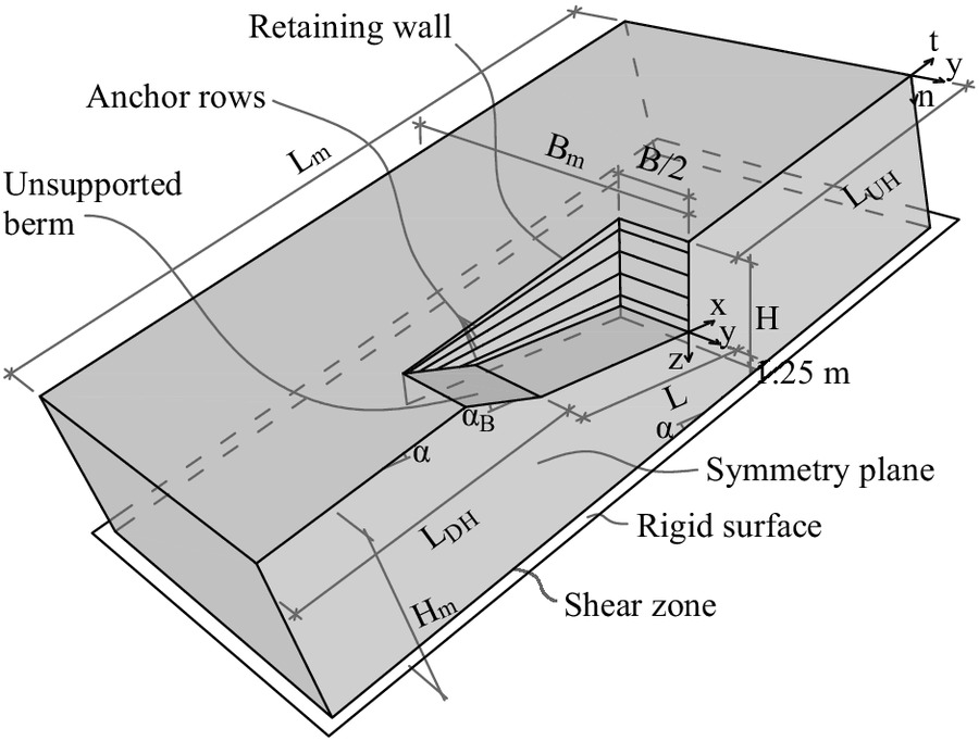
The following model design was used to account for these essential characteristics. The models consisted of a small landslide portion around the excavation pit in the form of an inclined rectangular block with dimensions

L_{m} \times B_{m} \times H_{m}

(Fig. 1). The block was bounded at the top by the terrain surface, at the bottom by the shear zone, and at the sides by appropriate boundary conditions. The intact ground below the shear zone was assumed to be rigid. The planar terrain and the shear zone were parallel to each other and inclined at an angle

α

. The strength of the shear zone was

φ_{s z}^{'} = α

, and the sliding body had a strength

φ^{'} > α

. Without the presence of groundwater, such a landslide has a safety factor of unity, allowing for the desired movement of the landslide mass along the shear zone during and after the excavation process. In active landslides, excavations below the phreatic surface are rare. Therefore, the presence of groundwater was neglected in the calculation of earth pressures on the retaining structure. Without explicitly including groundwater in the landslide model, its effects on the slope stability were considered implicitly by adopting the apparent value of

φ_{s z}^{'} = α

for the angle of friction in the shear zone, leaving the modeled landslide portion with a safety factor of unity. By prescribing the initial stress state, the modeled landslide portion can represent any location between the compression and the extension zones of the landslide. The boundary conditions and the initial stress state are discussed in detail in the following sections.

Excavation Pit

Fig. 1 shows the geometry and the layout of a representative excavation pit as it was assumed in this study. The main excavated volume had a cuboidal shape with length

L

, width

B

and height

H

at the uphill side. The orientation was such that two sides were parallel to the slope gradient. In the majority of the calculations the excavation pit was supported by retaining walls on three sides and by an unsupported berm on the downhill side. Only in a few calculations were there retaining walls on all four sides, and these cases are mentioned specifically. The geometry parameters of the landslide and the excavation are given in Table 1. They were chosen based on real landslide case studies in urban areas (e.g., Alonso et al. 2010; Puzrin and Schmid 2011; Oberender and Puzrin 2016).

Table 1. Landslide and excavation pit geometry parameters

Parameter	Description	Value
$H_{m}$ (m)	Height of landslide mass	20
$H$ (m)	Excavated depth on uphill side	10
$L$ (m)	Horizontal length of excavation pit	20
$B$ (m)	Width of excavation pit	20
$α$ (degrees)	Slope inclination	0, 10, 15, 20
$α_{B}$ (degrees)	Berm angle w.r.t. horizontal	$\min (0.95 \cdot α; 30 °)$

Constitutive Laws and Material Properties

Sliding Soil Mass

A widely used and accepted material model for soil modeling in engineering practice is the so-called Hardening Soil model, which is implemented in the commercial FE code PLAXIS 2018, and described by Schanz et al. (1999). For the calculations in the present work, the most important features of the Hardening Soil model were adopted and implemented as extensions into the built-in Mohr–Coulomb material model of Abaqus. The soil behavior followed the hyperbolic stress–strain relationship in drained triaxial shear loading proposed by Kondner and Zelasko (1963). This behavior was generated with an isotropic deviatoric frictional hardening rule for the Mohr–Coulomb type yield surface, with an equivalent plastic shear as a hardening parameter. Furthermore, the model incorporated stress-dependent stiffness for both virgin loading and elastic unloading and reloading. The volumetric behavior during yielding followed the stress-dilatancy theory of Rowe (1962, 1971) [revisited by Schanz and Vermeer (1996)], and was achieved using an appropriate nonassociated flow rule. The yield cap used in the Hardening Soil model was omitted here, because the consolidation process of the slope was not modeled. Table 2 contains the material parameters and their description, as well as the values used in this study. The values of

E^{ref}

,

p^{ref}

,

ν

,

φ_{f}^{'}

,

c^{'}

, and

γ

were chosen to be representative of realistic values inspired by real landslide cases in urban areas (e.g., Puzrin and Schmid 2011);

E_{50}^{ref}

,

ψ_{f}

, and

R_{f}

were derived and chosen as suggested by Schanz and Vermeer (1996, 1998) and Schanz et al. (1999). The value chosen for

m

represented clay, whereas sandier material usually has slightly lower values (von Soos and Bohac 2002). Nevertheless, it enabled a simple definition of the initial stress state, as well as the straightforward implementation of the material model into Abaqus.

Table 2. Soil material parameters

Parameter	Description	Value
$m$	Power for stress-level dependency of stiffness	1
$p^{ref}$ (kPa)	Reference stress for stiffness	100
$E^{ref}$ (MPa)	Elastic stiffness (Young’s modulus)	70
$ν$	Poisson’s ratio	0.3
$E_{u r}^{ref}$ (MPa)	Elastic stiffness in standard drained triaxial compression test	$3 E^{ref} / [2 (1 + ν)] = 80.77$
$E_{50}^{ref}$ (MPa)	Secant stiffness at 50% failure strain in a standard drained triaxial compression test	$E_{u r}^{ref} / 5 = 16.154$
$φ_{f}^{'}$ (degrees)	Mohr–Coulomb friction angle at failure	25, 30, 35
$ψ_{f}$	Dilation angle at failure	$φ_{f}^{'} / 3$
$R_{f}$	Failure ratio	0.9
$c^{'}$ (kPa)	Cohesion	$\approx 0$
$γ$ ( $kN / m^{3}$ )	Unit soil weight	20

Shear Zone

The shear zone, situated between the sliding soil mass and the stable ground, was modeled using a nondilatant interface with a contact constitutive law. The contact law was based on Coulomb friction with extensions for viscoplastic behavior. Viscosity was introduced as a form of damping to reach quasi-static equilibrium in a smooth fashion. In reality, the shear zone has a finite thickness, which in the model was taken into account by means of adequate elastic deformability both in normal and tangential directions. Normal stresses were calculated using the Kelvin–Voigt model (dashpot and spring in parallel), and the shear response was calculated using the Bingham–Hooke model (parallelized plastic slider and dashpot, in series with a spring). The frictional resistance of the slider followed the Coulomb friction model. The main parameters of the contact law are listed in Table 3. The values were inspired by real case landslides (e.g., Puzrin and Schmid 2011). The shear modulus

G_{s z}

was set rather low, for reasons of numerical stability, but the resulting impact was regarded to be negligible, because the whole shear zone was yielding perfectly plastic from the start of the simulation.

Table 3. Shear zone material parameters

Parameter	Description	Value
$t_{s z}$ (m)	Shear zone thickness	0.2
$G_{s z}$ (MPa)	Elastic shear modulus	1.6
$ν_{s z}$	Poisson’s ratio	0.25
$μ_{s z}$	Coefficient of friction	$\tan φ_{s z} = \tan α$

Excavated Soil Mass, Retaining Walls, and Soil Anchors

Due to the lack of an available built-in soil excavation modeling feature in Abaqus, a suitable material model was used for the soil to be excavated. The Drucker–Prager Cap model allows for defining a reduction of strength over time, down to practically zero. Simultaneously, the weight of the soil was removed, and the anchor forces were increased to their design values. At the end, the excavated soil carried no stresses, which is equivalent to the soil having been removed. This process of excavation occurred in one excavation stage, for reasons of simplicity. This simplification greatly reduced the degrees of freedom of the parametric study, and its implications on the results were limited. The global stability of the landslide was not altered, because the final anchor forces were the same. The wall deflections, on the other hand, might differ, but they will lie somewhere between the extremes resulting from more-realistically modeled excavation processes. A particularly unfavorable construction sequence with large excavation stages accompanied by minimal anchorage will generate larger wall deflections, whereas the opposite will result in smaller deflections. The chosen simplified approach therefore gave reasonably conservative results for excavation processes planned with adequate caution, as should be the standard when dealing with excavation in landslides. The adequacy of the modeling simplifications of the excavation process were further validated in the “Results and Discussion” section for excavations in stable slopes.

The retaining structure itself was a reinforced shotcrete wall with the geometry shown in Fig. 1. The wall-to-wall connections at the excavation pit corners were approximated as hinges. The walls were modeled using two-dimensional shell elements (S4), with an isotropic linear elastic material behavior. The geometric and the material parameters were chosen to be suitable for representing RC with a cracked section (Table 4). The interaction between retaining wall and surrounding soil was simulated by tying the wall nodes to the adjacent soil nodes. This realistically simulated the interaction between the rough shotcrete surface and the adjacent soil, in which any relative slip is likely to occur in the adjacent soil as plastic deformation.

Table 4. Retaining wall material parameters

Parameter	Description	Value
$t_{w}$ (m)	Retaining wall thickness	0.2
$E_{w}$ (GPa)	Young’s modulus	10
$ν_{w}$	Poisson’s ratio	0.2
$γ_{w}$ ( $kN / m^{3}$ )	RC unit weight	25

As is common in practice, the retaining wall was anchored with soil anchors placed in four rows at a regular spacing over the excavated height (Fig. 1). For simplicity, the anchor rows were modeled as horizontally acting line loads.

Boundary and Initial Conditions

Initial Stress State

This section presents the essential assumptions and definitions for the undisturbed stress state of a compressed landslide the complete derivations are given in Appendix S1 in the Supplemental Materials.

Part of the stress state of stable sloping ground, or an uncompressed landslide, can be described using an earth pressure coefficient

K_{0 h x} = \frac{σ_{x}}{γ \cdot z}

(1)

where

γ

= unit weight of soil;

z

vertical coordinate; and

σ_{x}

= normal stress at depth

z

acting on a vertical cut. In this work, the earth pressure coefficient for normally consolidated ground, proposed by Franke (1974) was used

K_{0 h x} = (1 - \sin φ^{'}) (1 + \sin α)

(2)

It is widely accepted in practice and has been calibrated with experiments, and both the Swiss code SIA (2020) and the European code CEN (2004) suggest its use. In a compressed landslide, the earth pressure is higher than that. According to Friedli et al. (2017) there is a maximum value which

K_{h x}

can reach, called the landslide pressure coefficient

K_{l h x}

K_{l h x} = \frac{σ_{x}}{γ z} = \frac{\cos^{4} α}{\cos^{2} φ^{'}} {[1 + \sqrt{1 - \cos^{2} φ^{'} (1 + \tan^{2} α)}]}^{2}

(3)

Assuming that landslides compress with roughly uniform

ε_{t}

over their depth

H_{m}

, which is suggested by the affinity of several deformation profiles from inclinometer measurements along the slide (e.g., Cevasco et al. 2018), together with the assumed linear stress dependency of stiffness, the compressed stress state can be described by an earth pressure coefficient

K_{h x}

. This coefficient consequently lies somewhere between

K_{0 h x}

and

K_{l h x}

, which leads to the definition of the landslide compression ratio

k_{c}

k_{c} = \frac{K_{h x} - K_{0 h x}}{K_{l h x} - K_{0 h x}}

(4)

In a compressed section of a landslide,

k_{c}

takes values between 0 and 1. A value of 0 represents an uncompressed landslide region with earth pressures identical to those of regular sloped ground (

K_{h x} = K_{0 h x}

), whereas

k_{c} = 1

describes a portion of a landslide being in a state of maximum compression (

K_{h x} = K_{l h x}

). Furthermore, although this was not considered in this work, values of

k_{c}

smaller than 0 also are possible when the earth pressure is below

K_{0 h x}

, e.g., as in extension zones of landslides.

Using Eqs. (1)–(4), and the complete derivations in Appendix S1 [specifically Eqs. (S13) and (S16)], most of the initial stress state is determined analytically for a specific

k_{c}

. Only the normal stress

σ_{y}

[Fig. 1 and Eq. (S13)] depends on the response of the soil during the compression process of the landslide, and it is not easily derived in a closed form. Therefore it was determined using a separate preliminary FE model, representing a one-element landslide compression process, starting from

K_{0}

conditions [Eq. (2)] up to the landslide pressure [Eq. (3)]. Initial values for

σ_{y}

(and also for the hardening parameter

ε_{s 0}^{p}

) for a specific

k_{c}

were taken from its output.

Static and Kinematic Boundary Conditions on the Landslide

The calculation model for the landslide portion, including the boundary conditions, is depicted schematically in Fig. 2. The sides and the downhill boundary were fixed in the normal direction. Furthermore, nodal forces, representing the shear stresses

τ_{t n}

, which remain constant over time, were prescribed on the downhill boundary. On the uphill boundary, nodal forces for both

τ_{t n}

and

σ_{t}

were prescribed;

σ_{t}

also remained constant, because no increase in compression of the landslide during the excavation process was considered. The contact interaction, representing the shear zone behavior, acted between the soil at the shear zone model boundary and a fixed plane, representing the stable ground below the sliding mass. The initial contact forces in the shear zone, which are necessary for the equilibrium of the landslide before the excavation, were prescribed as nodal forces. They were taken into account in the contact response calculation. Finally, the initial internal stress state and the initial value of the hardening parameter

ε_{s 0}^{p}

were prescribed for all elements.

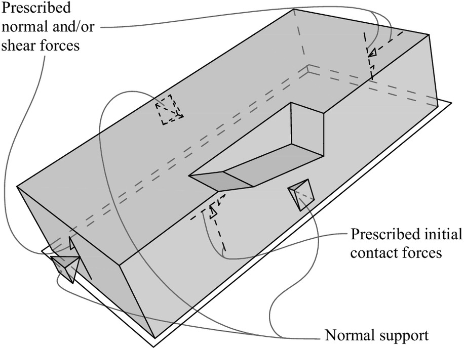
Fig. 2. Kinematic and static boundary conditions.

The values for the preceding static boundary conditions, for every boundary node, were determined using a preliminary FE model with identical geometry. All nodes were fixed, and the initial stress state was imposed using the corresponding user subroutine. The output reaction forces at the boundary of this model were the desired static boundary condition for the main calculation model.

Ultimately, the chosen system of boundary conditions enabled the aforementioned essential landslide characteristics. The static boundary condition on the uphill boundary allowed for downhill movement during the excavation process, whereas the boundary stresses remained constant and the far field in the uphill direction was preserved. The normally supported downhill boundary, on the other hand, represented the stabilizing part of the landslide, and was able to resist an unbalanced force, possibly arising due to the excavation. This setup, although unsuitable to predict global landslide movements, should allow for a reasonable prediction of the local displacement field around an excavation pit within a landslide.

Anchor Prestressing Forces

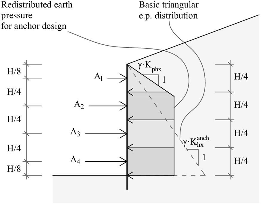
For excavations in stable ground (i.e., no landslide), the following applies as common practice for the design of rather stiff retaining walls with multiple rows of prestressed anchors: Deutsche Gesellschaft für Geotechnik e.V. (2012) proposes generally to consider active earth pressures, unless buildings are present in the influence zone of the excavation. In that case, increased active earth pressure, ranging as high as earth pressure at rest, should be taken into consideration, depending on the distance and susceptibility of the neighboring buildings. The corresponding distribution of the earth pressure depends strongly on the construction procedure and sequences, and on the prestressing forces of the anchors. A very simple, trapezoidal distribution was proposed by Terzaghi (1941). Deutsche Gesellschaft für Geotechnik e.V. (2012) proposes variations thereof, depending on how close the chosen pressure is to the at-rest earth pressure. In general, the smaller the retaining wall deflections, the closer the earth pressure is to at-rest pressures without significant redistribution from a triangular to a trapezoidal shape. Nevertheless, using a triangular at-rest earth pressure distribution for determining the anchor prestressing forces is not sufficient to keep deformations to a minimum. The smallest possible construction stages also are required. Otherwise, during each stage the unsupported part experiences significant deformations. Deutsche Gesellschaft für Geotechnik e.V. (2012) uses a proportion factor to express the magnitude of increased active earth pressure. For anchor design, using horizontal earth pressure coefficients, it is

f_{a - 0}^{anch} = \frac{K_{h x}^{anch} - K_{a h x}}{K_{0 h x} - K_{a h x}}

(5)

where

f_{a - 0}^{anch}

takes values between 0 and 1;

K_{a h x}

= active horizontal earth pressure coefficient, which in this study was taken according to Coulomb (1776), with interface friction

δ_{a} = \frac{2}{3} φ^{'}

; and

K_{h x}^{anch}

= horizontal earth pressure coefficient considered for determining the anchor pre-stressing forces.

For the case of an excavation in a landslide, it is a more difficult task to design a retaining wall. First, the state of compression in a landslide often is close to unknown. The earth pressure may lie anywhere between the active and the passive landslide pressure (Friedli et al. 2017). Secondly, no well-founded guidelines presently exist with information on earth pressure magnitude and distribution for determining anchor prestressing forces which will result in acceptable performance of the retaining structure in terms of deformations. Therefore, in this study, various earth pressure magnitudes for anchor design were considered for many different compression ratios

k_{c}

of the landslide. For the main part of the study, the assumed earth pressure distribution for the anchor design was a very simple, slight variation of the original trapezoidal distribution (Fig. 3). The earth pressure near the surface is limited by the passive earth pressure, according to Caquot and Kérisel (1948, 1949) (assuming zero interface friction), to a certain depth from at which earth pressures remain constant. The resultant of the redistributed earth pressure is equal in magnitude to the resultant of the basic triangular distribution. The anchor force of each anchor row corresponds to its share of earth pressure over the height, neglecting anything below the excavation base. Full earth pressure redistribution was considered for all cases, even when the anchor was designed for the modeled in situ pressure, because in reality, unlike in the numerical model, the in situ pressure is unknown. To express the amount of earth pressure considered for the anchor design in the case of a landslide, one more factor is defined

f_{0 - l}^{anch} = \frac{K_{h x}^{anch} - K_{0 h x}}{K_{l h x} - K_{0 h x}}

(6)

where

f_{0 - l}^{anch}

is similar to landslide compression ratio

k_{c}

[Eq. (4)], and takes values between 0 and 1.

Fig. 3. Earth pressure distribution considered for anchor design.

FE Model Progression

The calculation was carried out in two stages. First, the retaining wall was introduced by increasing its weight. The subsequent stage consisted of the excavation of the soil and the simultaneous introduction of the anchor forces.

Postprocessing of the Results

The governing factors for damage to buildings have been a subject of extensive research. Early work was done to relate settlement under self-weight to building damage reported from observations (Skempton and MacDonald 1956; Polshin and Tokar 1957). It became clear that differential settlement with vertical deflection plays a governing role. Burland and Wroth (1974) formulated definitions for the deformation of foundations, such as the deflection ratio. These have been used widely by other authors. Furthermore, Burland and Wroth concluded that visible cracking was a result of excessive tensile strains, and they presented the limiting tensile strain method, which allows for relating settlement to the maximum extreme tensile fiber strain in a building wall by approximating the building walls as isotropic bending and shear beams. In contrast to the purely vertical settlement under self-weight, ground deformations next to a construction site with a deep excavation consist of vertical settlement mixed with horizontal extension (Boscardin and Cording 1989). Therefore, Boscardin and Cording extended the limiting tensile strain method to account for the superposition of bending and shear with tension. A slightly modified version was adopted subsequently by Burland (1995). Boscardin and Cording (1989) also related the maximum extreme tensile strains from the limiting tensile strain method to building damage. They used damage categories of the severity of cracking that were developed by Burland et al. (1977). Son and Cording (2005) suggested slightly adapted tensile strains for the boundaries of the same damage categories. The damage categories and boundary tensile strains are given in Appendix S2 in the Supplemental Materials.

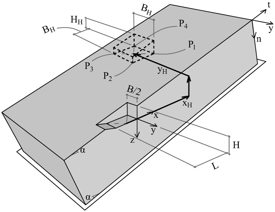
The direct output of the FEM calculations carried out in this work were the deformations around the excavation site, without any buildings present in its vicinity. Applying the limiting tensile strain method directly to these so-called greenfield deformations is conservative, because buildings resist deformation to a certain extent, depending on their stiffness and interaction properties with the soil (Burland 1995). Nevertheless, the approach is useful for a broad estimation of the damage influence zone around a deep excavation. A more detailed, and therefore rather intricate, examination might be beneficial for buildings situated in the zone of considerable damage. However, as mentioned previously, this is especially difficult for investigations within a landslide. To apply the limiting tensile strain method to a large area around the excavation pit of each model, the greenfield deformations obtained from the FEM calculations were postprocessed. Possible positions of neighboring buildings were defined by their relative position to the excavation pit

(x_{H}, y_{H})

(Fig. 4). The buildings had a horizontal, square footing of width

B_{H}

, with corner points

P_{1}

,

P_{2}

,

P_{3}

, and

P_{4}

and an embedment

H_{H}

on the uphill side. Table 5 lists the geometric building parameters and their values. Furthermore, definitions of the relative deflection, the deflection ratio and the average horizontal direct tensile strain are given, and an explanatory visualization is shown in Fig. 5(a). These quantities were calculated from the excavation-induced displacements of the four corner points, for each of the four basement walls of the building (

P_{1} - P_{2}

,

P_{2} - P_{3}

,

P_{3} - P_{4}

, and

P_{4} - P_{1}

). The deflection ratio of each wall was evaluated at the midspan and both third-span points, and only the maximum of the three was considered further. For vertical deflection, there are two different deformation modes, called sagging and hogging [Fig. 5(b)], to which the building reacts differently. Therefore, the deflection ratio was evaluated separately for the sagging and the hogging modes.

Fig. 4. Definition of neighboring building position $(x_{H}, y_{H})$ , measured between the center points of the excavation and the basement slab.

Table 5. Building geometry and deformation parameters

Parameter	Description	Value
$B_{H}$ (m)	Undeformed width of building	20
$B_{H}^{'}$	Deformed width of building	—
$H_{H}$ (m)	Uphill embedment of building	10
$Δ_{1}$ , $Δ_{2}$ , $Δ_{3}$	Relative deflection at midspan and both third-span points of building wall	—
$\tilde{Δ}$	Deflection ratio	$[\max (Δ_{1}, Δ_{2}, Δ_{3})] / B_{H}$
$ε_{t}$	Average horizontal direct tensile strain	$(B_{H}^{'} - B_{H}) / B_{H}$
$ε_{c}$	Average horizontal direct compressive strain	$(B_{H} - B_{H}^{'}) / B_{H} = - ε_{t}$

Fig. 5. (a) Evaluated relative deflections of a building; and (b) sagging versus hogging deformation modes.

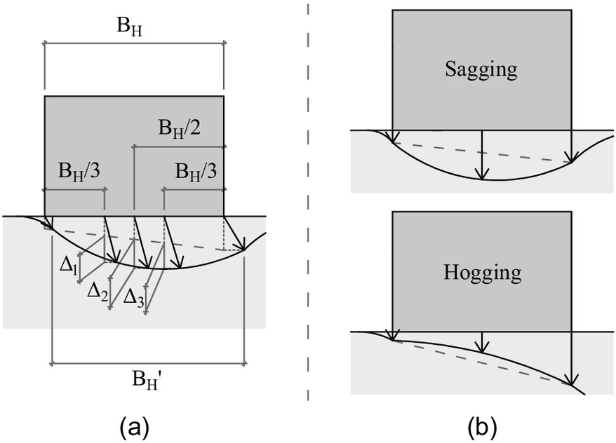
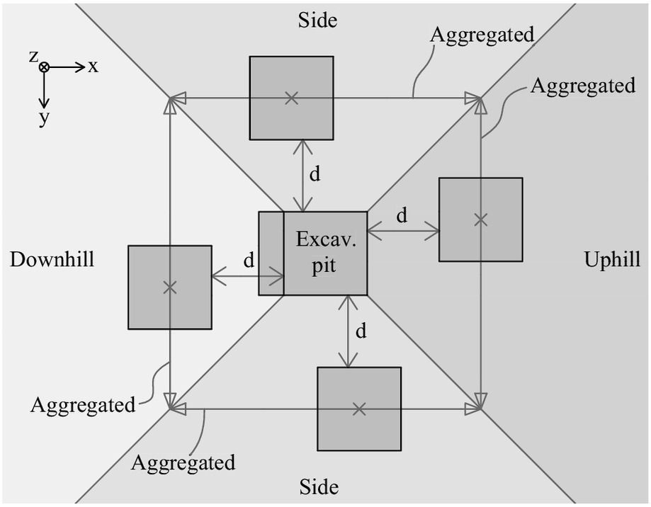
For each of the four building walls, the maximum tensile strain method was applied, according to Burland and Wroth (1974), Burland et al. (1977), and Burland (1995). The alteration of using a shear factor

t_{f a c}

of 1.2 instead of 1.5, suggested by Netzel (2005), was adopted. The resulting formulas for the calculation of the total maximum tensile strain

ε_{\max}^{tot}

are

ε_{h} = \frac{\tilde{Δ}}{\frac{\frac{B_{H}}{h_{H}}}{12 \cdot \frac{z_{b}}{h_{H}}} \cdot (1 + t_{f a c} \cdot 12 \cdot \frac{E_{H}}{G_{H}} \cdot \frac{I_{H}}{h_{H}^{3}} \cdot {(\frac{h_{H}}{B_{H}})}^{2})}

(7)

ε_{h}^{tot} = ε_{t} + ε_{h}

(8)

ε_{d} = \frac{\tilde{Δ}}{1 + \frac{{(\frac{B_{H}}{h_{H}})}^{2}}{t_{f a c} \cdot 12 \cdot \frac{E_{H}}{G_{H}} \cdot \frac{I_{H}}{h_{H}^{3}}}}

(9)

ε_{d}^{tot} = ε_{t} \cdot \frac{1 - ν_{H}}{2} + \sqrt{{(ε_{t} \cdot \frac{1 + ν_{H}}{2})}^{2} + ε_{d}^{2}}

(10)

ε_{\max}^{tot} = \max (ε_{h}^{tot}, ε_{d}^{tot})

(11)

Descriptions and parameter values used in the calculations are given in Table 6. The parameter values were chosen in accordance with Burland and Wroth (1974) and Netzel (2005). A value of 1 was chosen as a generalized estimate of the length to height ratio

B_{H} / h_{H}

of the building walls. However, in reality a rather broad range can be expected to exist, depending on the exact building properties. The

E_{H} / G_{H}

ratio,

z_{b} / h_{H}

, and therefore

I_{H} / h_{H}^{3}

, are different for the sagging and the hogging modes, as suggested by Burland and Wroth (1974) and Netzel (2005). Finally, in general, the highest value of

ε_{\max}^{tot}

for hogging or sagging and for each of the four walls was considered in the evaluation of the building’s damage potential. For better understanding, the individual

ε_{\max}^{tot}

components were sometimes considered separately (e.g., only slope parallel or lateral walls, or only sagging or hogging). The whole procedure was carried out for a fine grid of possible house locations

(x_{H}, y_{H})

. For visualization and comparability, the results on the grid subsequently were aggregated further. Three sectors around the excavation pit were defined—uphill, side, and downhill (Fig. 6)—for which the results were processed separately. Within each of these sectors, buildings with the same clear distance

d

to the excavation pit (orthogonally) were aggregated, and only the respective maximum was considered. A normalized clear distance

\hat{d} = d / B

was introduced for displaying the results.

Table 6. Parameters of limiting tensile strain method and their description

Parameters	Description	Values used
Parameters	Description	Sagging	Hogging
$B_{H}$ , $h_{H}$	Length and height of building wall	$B_{H} / h_{H} = 1$
$t_{f a c}$	Timoshenko shear factor	1.2
$ν_{H}$	Poisson’s ratio of wall	0.3
$E_{H}$ , $G_{H}$	Young’s modulus and shear modulus of wall	$E_{H} / G_{H} = 2.6$	$E_{H} / G_{H} = 0.5$
$z_{b}$	Distance (from top of wall) of neutral axis for bending	$z_{b} / h_{H} = 0.5$	$z_{b} / h_{H} = 1$
$I_{H}$	Second moment of area of wall for bending from vertical deflection	$I_{H} / h_{H}^{3} = 1 / 12$	$I_{H} / h_{H}^{3} = 1 / 3$
$ε_{h}$	Maximum horizontal tensile strain from vertical deflection alone	—	—
$ε_{h}^{t o t}$	$ε_{h}$ superimposed with horizontal extension $ε_{t}$	—	—
$ε_{d}$	Maximum diagonal tensile strain from vertical deflection alone	—	—
$ε_{d}^{tot}$	$ε_{d}$ superimposed with horizontal extension $ε_{t}$	—	—
$ε_{\max}^{tot}$	Total maximum tensile strain	—	—

Fig. 6. Definition of three sectors (uphill, side, and downhill), and aggregation of results along lines with the same clear distance $d$ to the excavation pit, within each sector separately.

For building wall materials, compressive strains generally are less harmful than tensile strains. Moreover, because this problem does not occur in the literature, excavation in stable ground does not seem to generate significant compressive strains on neighboring building walls. Within landslides, however, compressive strains seem to be a plausible risk for buildings near excavation pits, because the sliding mass can move with respect to the stable zone below. Therefore, in addition to tensile strains, compressive strains also were evaluated as average horizontal direct compressive strains

ε_{c}

(Table 5).

Layout of the Parametric Study

The parametric study was designed to cover a realistic range of

α - φ^{'}

combinations for landslides containing built-up areas. The location of the excavation pit within the landslide was taken into account by varying

k_{c}

. To account for the lack of knowledge of

k_{c}

in reality, anchor design factors

f_{0 - l}^{anch}

or

f_{a - 0}^{anch}

also were varied. Table 7 gives the parameters that were varied and their values, and Appendix S3 in the Supplemental Materials contains more-detailed information of all the models run for the study. Fig. S2 in the Supplemental Materials shows all the calculated landslide model variations. For reference, a series of models with an excavation within a stable slope also was calculated (Fig. S3). The models on stable flat ground each were run once with a berm on the downhill side, and once with a retaining wall on all four sides of the excavation (Fig. S4). Another limited model series was run for reference, with stable slopes and anchor design for the full

K_{0}

earth pressure, but with the anchor designed for a triangular earth pressure distribution (Fig. S5).

Table 7. Parameters varied in parametric study and their values

Parameter	Description	Value
$α$ (degrees)	Slope inclination	0, 10, 15, 20
$φ^{'}$ (degrees)	Mohr-Coulomb friction angle at failure	25, 30, 35
$k_{c}$	Landslide compression ratio	0, 0.2, 0.4, 0.6, 0.8, 1
$f_{0 - l}^{anch}$	Anchor design factor	0, 0.2, 0.4, 0.6, 0.8, 1 but $\leq k_{c}$
$f_{a - 0}^{anch}$	Anchor design factor for increased active earth pressure	0.25

Results and Discussion

The damage categories used are described and the tensile strain boundaries are given in Appendix S2.

The Figures in this section provide information about the expected damage potential to a neighboring building at varying distance from the excavation. They should, for a wide variety of cases, enable a designer to choose the proper level of excavation support that will result in an acceptably small impact on neighboring buildings.

Stable Slopes

The results in this subsection serve as a validation of the excavation modeling procedure, and were used as a reference for assessing the data from excavations within landslides. Fig. 7(a) represents cases with an ideal anchor design, i.e., with anchors designed to compensate for the full amount of in situ earth pressure (

f_{0 - l}^{anch} = k_{c} = 0

). However, there appears to be a significant potential for damage in the uphill sector for certain cases, and in the downhill sector for the cases in which

α = 0

. As previously mentioned, when fully compensating for the in situ earth pressures with the anchors, it could be beneficial to consider a triangular earth pressure distribution for the anchor prestressing, rather than some form of earth pressure redistribution. The damage potential to neighboring buildings in the uphill sector was reduced to negligible values when anchors were prestressed according to a triangular earth pressure distribution, compared with a trapezoidal redistribution (Fig. 8). The side sector also had very slight improvement, whereas the downhill sector remained unaffected. The downhill side of the excavation pit was modeled here as an unsupported berm. For a constant excavated depth

H

and a constant horizontal length of the excavation pit

L

, the unsupported berm height was larger for smaller

α

. The damage potential increased with decreasing

α

(i.e., increasing berm height) [Fig. 7(a)]. For the cases studied, there was potential for damage only for

α = 0

. Nevertheless, although for inclined ground it is common to realize the downhill side with an unsupported berm, this is not the case for flat terrain. For cases with

α = 0

, changing from a berm to an anchored retaining wall on the downhill side eliminated the damage potential in the downhill sector, whereas the uphill and the side sectors remained practically unaffected (Fig. 9). The kink in the line with

α = 0

,

φ^{'} = 25 °

and

f_{a - 0}^{anch} = 0.25

in the downhill sector of Fig. 7 was due to the fact that the unsupported berm of this height was only barely stable, and some localized shear deformation occurred there. It can be concluded that when fully compensating for the in situ earth pressure with anchors, it is possible to avoid damage to neighbors entirely.

Fig. 7. $ε_{\max}^{tot}$ versus $\hat{d}$ for stable slope cases, with a distinction between the different sectors: (a) $f_{0 - l}^{anch} = 0$ ; and (b) $f_{a - 0}^{anch} = 0.25$ .

Fig. 8. $ε_{\max}^{tot}$ versus $\hat{d}$ for stable slope cases with $f_{0 - l}^{anch} = 0$ and $φ^{'} = 30 °$ : comparison of trapezoidal and triangular earth pressure distribution for anchor design, with a distinction between the different sectors.

Fig. 9. $ε_{\max}^{tot}$ versus $\hat{d}$ for cases on stable flat ground ( $α = 0$ ), with a distinction between the different sectors and $f_{0 - l}^{anch} = 0$ or $f_{a - 0}^{anch} = 0.25$ : comparison of unsupported berm or retaining wall on the downhill side.

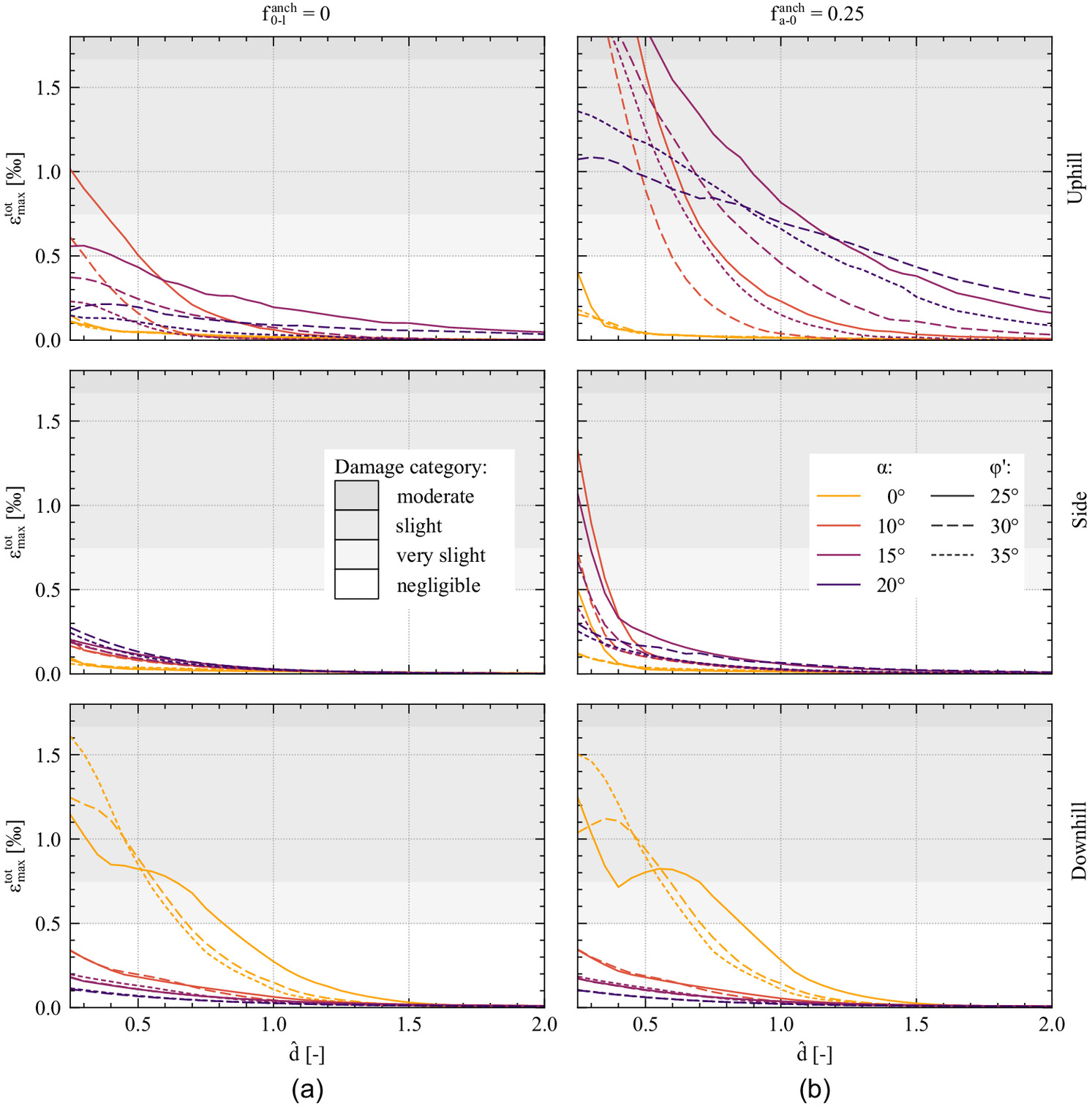
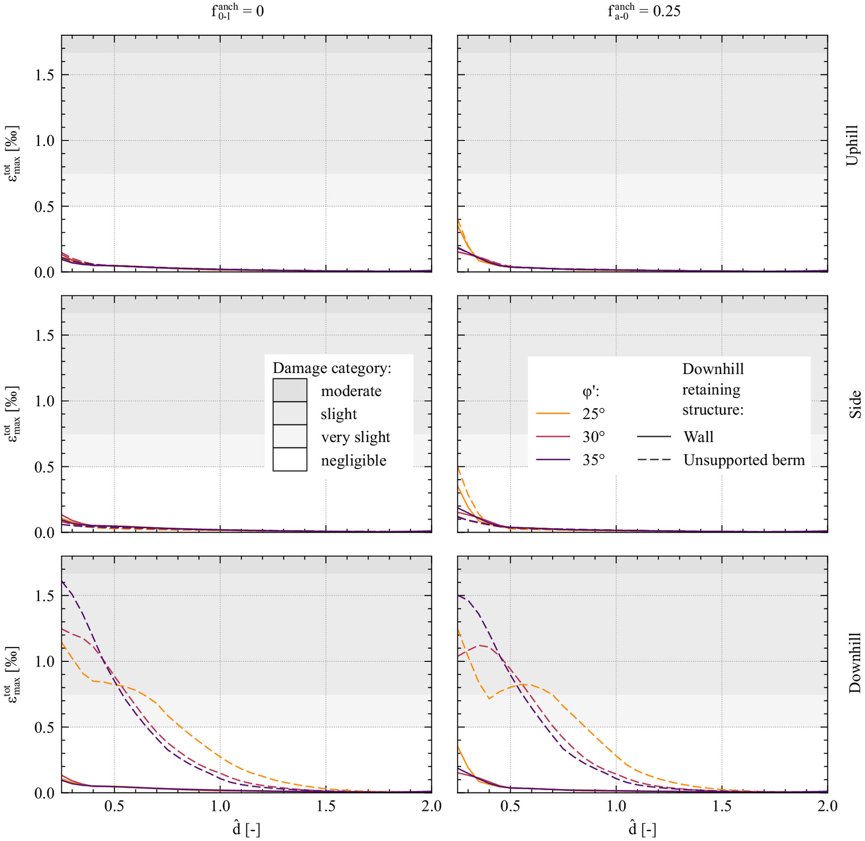
Fig. 7(b) implies that for sloped ground in contrast to flat terrain, designing anchors for increased active earth pressure generates a significant damage potential for neighbors, especially in the uphill sector. At first glance, the shape and the magnitude of the lines of

ε_{\max}^{tot}

relative to each other is not intuitively comprehensible. An explanation is given in Appendix S4.

The findings in this subsection are in accordance with the suggestions by Deutsche Gesellschaft für Geotechnik e.V. (2012): there is a potential for damage to close neighbors when the anchors are designed for increased active earth pressure, whereas an anchor design for earth pressure at rest with a triangular distribution eliminates the damage potential. This validates the simplifications chosen for the excavation modeling procedure used in this study.

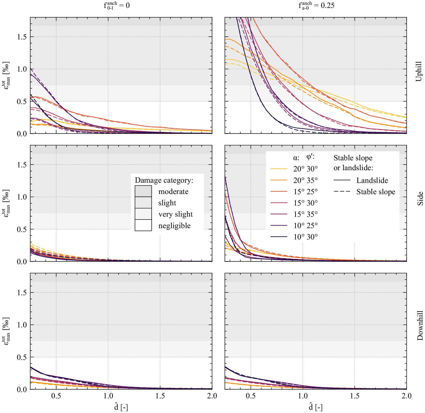
Comparison of Stable Slopes and Landslides

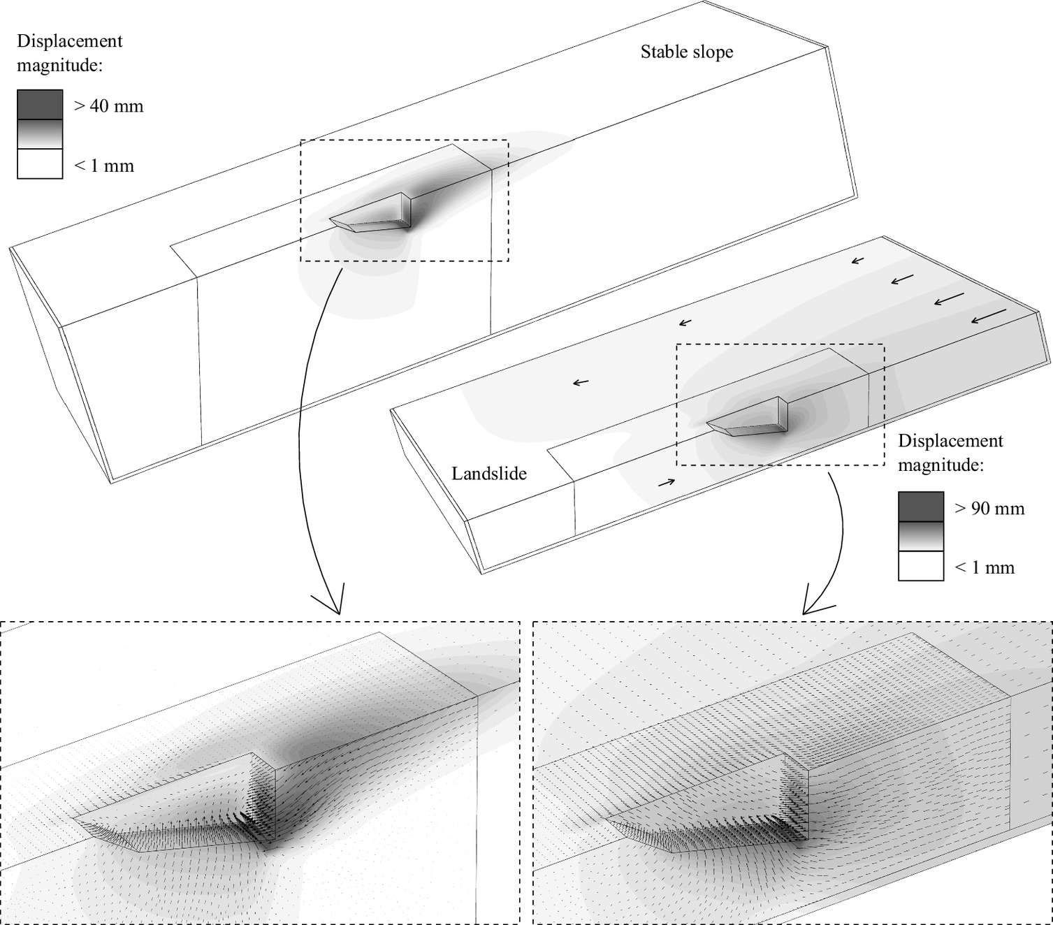
Comparison of stable slopes and uncompressed

(k_{c} = 0)

landslides (Fig. 10) reveals that for the cases studied and the geometries chosen, there is practically no difference for

ε_{\max}^{tot}

around excavations, independent of the anchor design. Conversely, excavations in compressed landslides

(k_{c} > 0)

, on the other hand, do generate a fundamentally different displacement field. Fig. 11 shows qualitatively representative displacement fields for a stable slope and a compressed landslide. The reach of the zone of significant displacements (e.g.,

> 1 mm

) around an excavation in a stable slope remains rather limited, whereas in a compressed landslide a more global movement of the landslide part uphill of the excavation pit along the shear zone in downhill direction can be evoked.

Fig. 10. $ε_{\max}^{tot}$ versus $\hat{d}$ , with a distinction between the different sectors and $f_{0 - l}^{anch} = 0$ or $f_{a - 0}^{anch} = 0.25$ : comparison of stable slope cases and uncompressed landslides $(k_{c} = 0)$ .

Fig. 11. Representative displacement field (magnitude and direction) of an excavation within a stable slope versus a compressed landslide $(k_{c} = 0.8)$ with $α = 15 °$ , $φ^{'} = 25 °$ and $f_{a - 0}^{anch} = 0.25$ .

Compressed Landslides

Downhill Sector

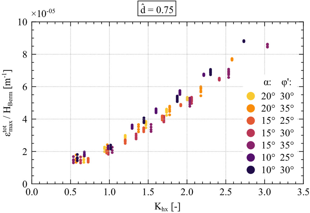
Fig. 12 shows the results of

ε_{\max}^{tot}

versus the normalized clear distance

\hat{d} = d / B

in the downhill sector. For every combination of

(α, φ^{'}, k_{c})

the range of

ε_{\max}^{tot}

is shown for various anchor design coefficients

K_{h}^{anch}

; the dashed and solid lines mark the lower and upper boundaries, respectively. The results show that for one combination of

(α, φ^{'}, k_{c})

,

ε_{\max}^{tot}

was independent of the anchor design, and for one set of

α

and

φ^{'}

a higher landslide compression

k_{c}

led to higher

ε_{\max}^{tot}

. This was because the ground deformation is a result of the complete unloading of the unsupported soil at the berm surface. An example of the resulting displacement field is depicted in Fig. 11. A higher

k_{c}

value will lead to a greater unloading and therefore larger displacements. The same is true for a higher unsupported height

H_{Berm}

of the berm. Fig. 13 confirms this trend, using

K_{h x}

instead of

k_{c}

. Finally, for high landslide compression ratios

k_{c}

and large unsupported heights

H_{Berm}

(i.e., small

α

), there is a potential for damage to close neighbors (i.e.,

\hat{d} < 0.8

) (Fig. 12). In those cases, a less-inclined berm might help, although this was not examined in this study. Apart from this, supporting the excavation with a retaining wall on all four sides could be a possible solution if the space is too limited for a less-inclined berm.

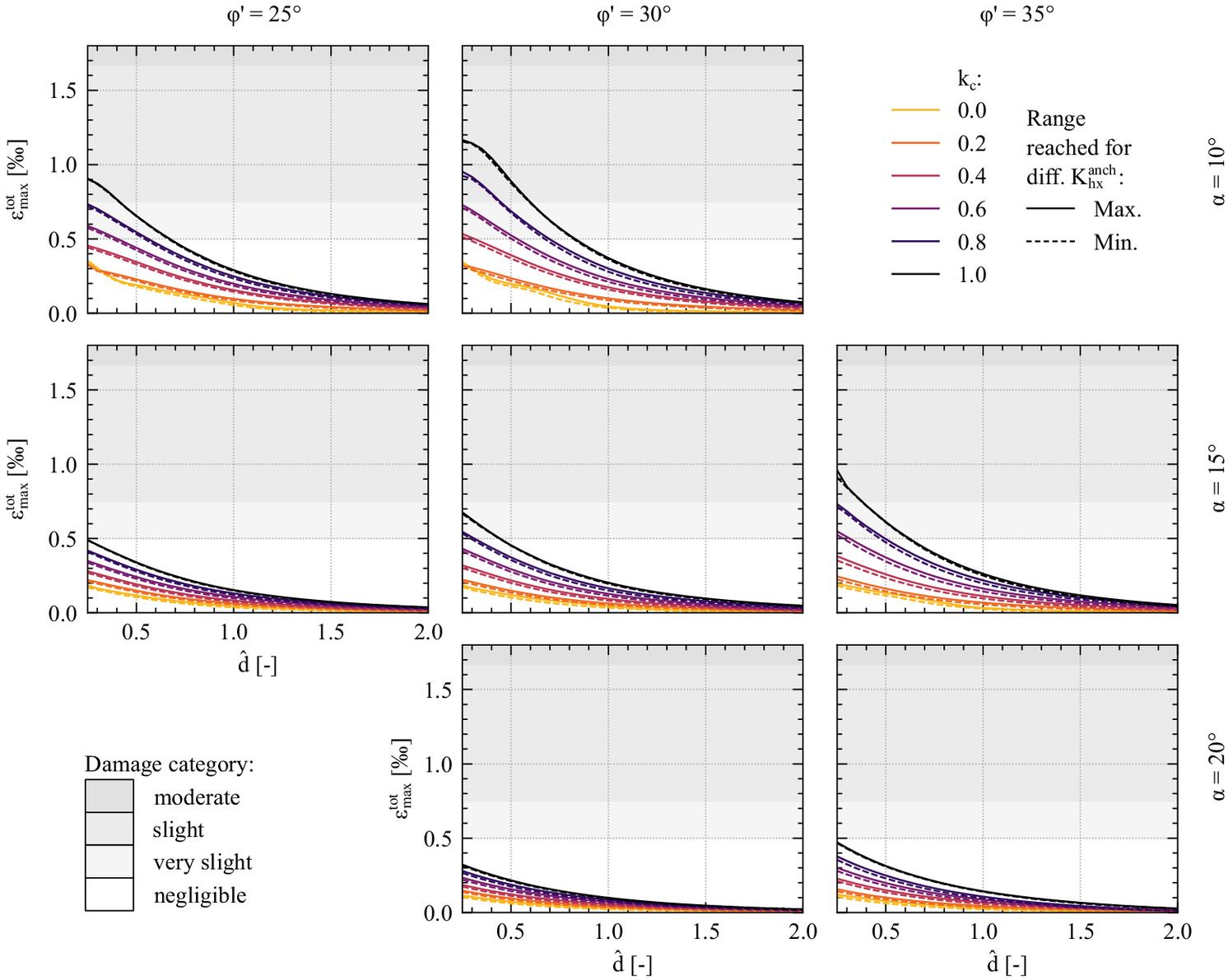
Fig. 12. $ε_{\max}^{tot}$ versus $\hat{d}$ in the downhill sector for the landslide cases, with a distinction between different values of $φ^{'}$ and $α$ .

Fig. 13. $ε_{\max}^{tot} / H_{Berm}$ versus $K_{h x}$ in the downhill sector at $\hat{d} = 0.75$ , for the landslide cases.

Side Sectors

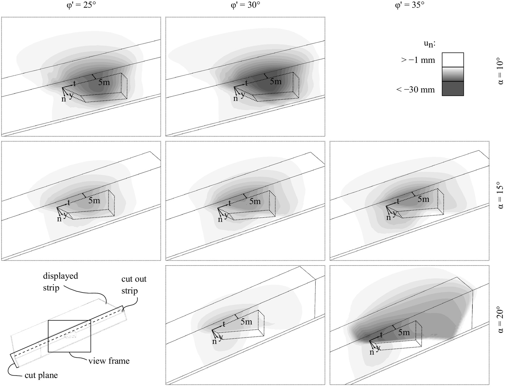
Fig. 14 shows the results of

ε_{\max}^{tot}

versus the normalized clear distance

\hat{d}

in the side sector. For every combination of

(α, φ^{'}, k_{c})

the range of

ε_{\max}^{tot}

is shown for various anchor design coefficients

K_{h}^{anch}

; the dashed and solid lines mark the lower and upper boundaries, respectively. Models with

k_{c} = 1

are displayed separately, because these models were not evaluated for the same range of anchor designs, and, more importantly, their results somewhat fall out of line. The results show that the damage potential of landslides with

k_{c} < 1

for neighboring buildings in the side sector was significant, but had quite a small reach. Buildings farther than

\hat{d} > 0.5

should not be expected to experience damage. Low anchor design coefficients (solid lines) should be avoided for certain landslides in the case of close neighbors, whereas with high anchor design coefficients (dashed lines) damage will always be prevented. Of all the studied landslides with

k_{c} = 1

, the case with

α = 20 °

and

φ^{'} = 35 °

had a distinctly higher damage potential (at least for

f_{0 - l}^{anch} < k_{c}

). This is explained in Fig. 15. For an anchor design

f_{0 - l}^{anch} = 0.4

, only the landslide with

α = 20 °

and

φ^{'} = 35 °

developed a very distinct moving wedge with localized deformation planes extending in the range of 20 m to the side of the excavation. In the other cases, the

u_{n}

-displacements evolved more gradually around the excavation, although not necessarily with lower magnitudes or extent. The profile of the distinct moving wedge strongly resembles that proposed by Friedli et al. (2017) for the maximum compression state of a landslide. Investigation of the conditions that lead to the formation of such a moving wedge when excavating in a landslide with

k_{c} = 1

was out of scope of this work. Nevertheless, it can be concluded that for landslides with

k_{c} = 1

there is a potential for large damage when not fully compensating for the in situ earth pressure with the anchor design.

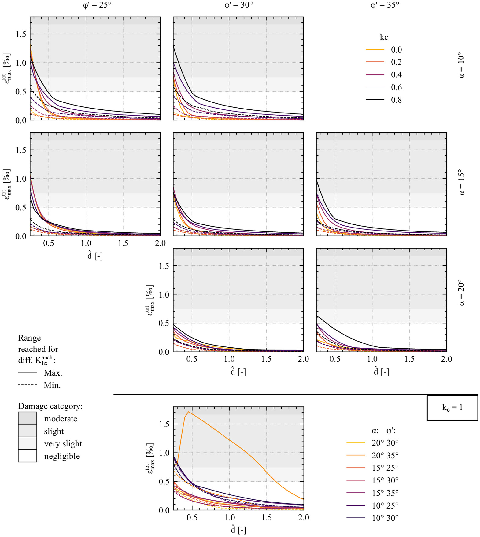
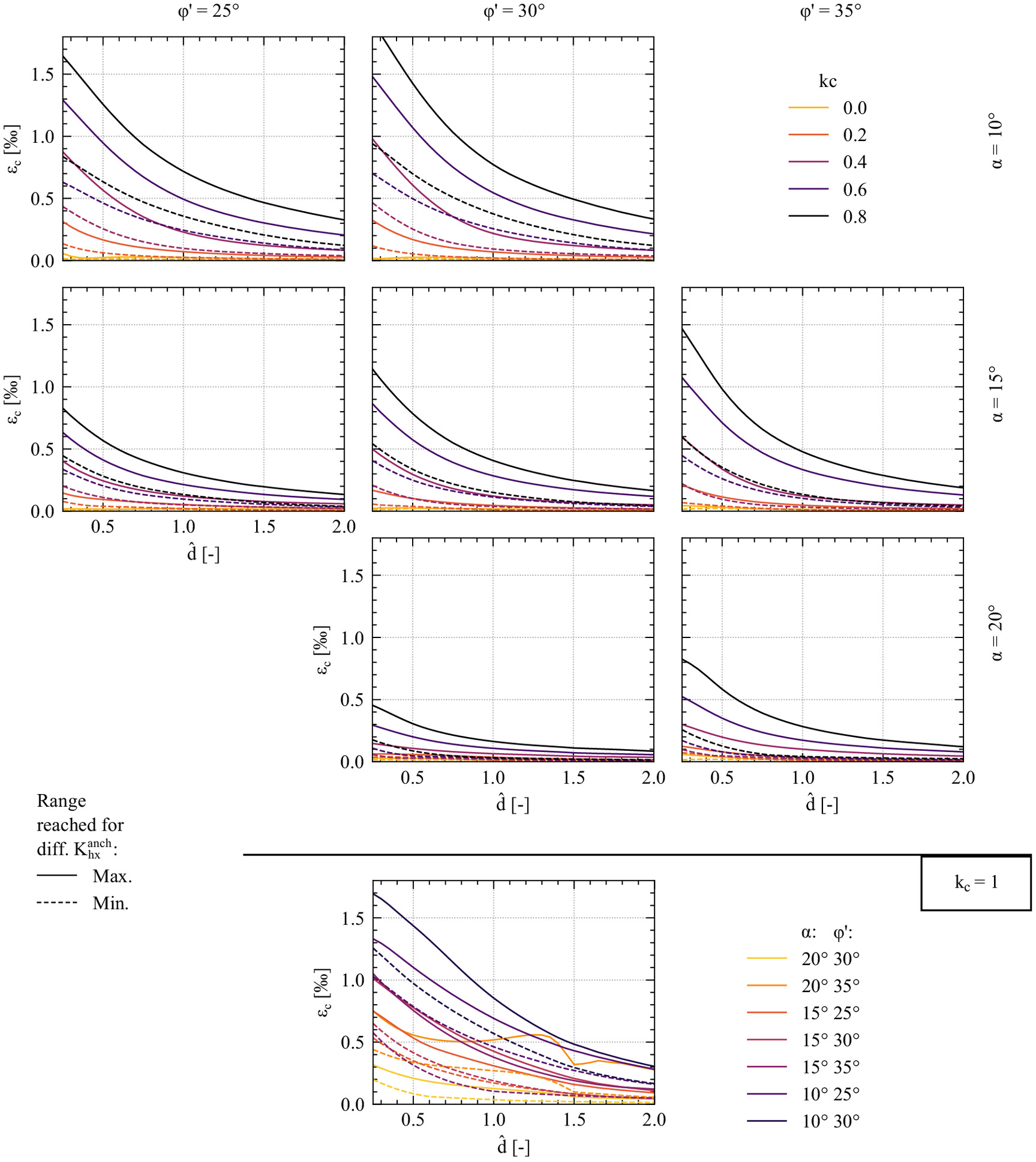
Fig. 14. $ε_{\max}^{tot}$ versus $\hat{d}$ in the side sector for the landslide cases, with a distinction between different $φ^{'}$ and $α$ ; cases with $k_{c} = 1$ are shown separately.

Fig. 15. Displacement component $u_{n}$ for 7 landslides with $k_{c} = 1$ and $f_{0 - l}^{anch} = 0.4$ . Vertical cut $5 m$ next to the excavation.

In addition to tensile strains

ε_{\max}^{tot}

as a result of bending and extension of the building walls, the deformation field predicted an overall compressive strain

ε_{c}

for some of the walls. Although for classical non-landslide problems (i.e., building deformations due to self-weight or deep excavations) direct compressive strains do not develop significantly, they do occur in landslides. Fig. 16, analogous to Fig. 14 but for the slope-parallel

ε_{c}

, instead of

ε_{\max}^{tot}

, shows that

ε_{c}

is larger for higher

k_{c}

and lower anchor design

f_{0 - l}^{anch}

, and depends on the landslide parameters

α

and

φ^{'}

. For

k_{c} = 1

, there is the same irregularity for the landslide with

α = 20 °

and

φ^{'} = 35 °

as for

ε_{tot}^{\max}

, although not as pronounced. The literature lacks a method for predicting building damage due to compressive strain calculated from greenfield deformations, and an extensive investigation was out of scope of this work. Nevertheless, some calculations are presented to give a roughly estimated indication of the damage potential.

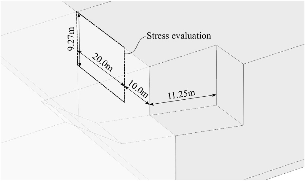
Fig. 16. $ε_{c}$ slope parallel versus $\hat{d}$ in the side sector for the landslide cases, with a distinction between different $φ^{'}$ and $α$ ; cases with $k_{c} = 1$ are shown separately.

Firstly, the evolution of the stresses

σ_{x}

in the side sector next to the excavation were investigated, in order to estimate the order of magnitude of the stress increase that accompanies the occurring compressive strains

ε_{c}

. This was carried out on the landslide model with

α = 10 °

,

φ^{'} = 30 °

,

k_{c} = 0.6

, and

f_{a - 0}^{anch} = 0.25

. A plane cut of roughly the size of the neighboring building’s embedment on its uphill side was chosen next to the excavation pit. On this cut, the stresses were compared before and after the excavation. Fig. 17 shows the cut and its location. The embedment depth was close to 10 m when fitting to the FEM mesh. The ratio

(K_{h x}^{end} - K_{h x}^{start}) / K_{0 h x}

quantifies the resulting stress increase, expressed as a relative increase of the horizontal earth pressure coefficient with respect to

K_{0 h x}

, and was

+ 14 %

for the investigated case. Keeping in mind that it was determined on the basis of greenfield deformations and assuming that a real building would be stiffer than the soil in its place, one can argue that the real stress increase acting on the building will be higher than the determined 14%, which certainly is significant and could lead to damage to the building.

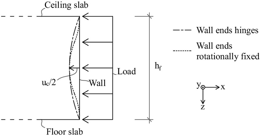
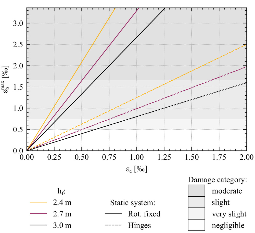
Fig. 17. Cut next to the excavation pit for the evaluation of the stress increase during the excavation.

Secondly, the effect of imposing the greenfield compressive strain

ε_{c}

on the building was examined. For that,

ε_{c}

is converted into a displacement

u_{c} = ε_{c} \cdot B_{H}

, and

u_{c} / 2

was applied in out-of-plane bending to the building’s basement wall. The simplifying assumptions were that the load transfer occurred only vertically over the floor height

h_{f}

, and

u_{c} / 2

is the horizontal deflection at midheight under a uniformly distributed load. The wall thickness was assumed to be 150 mm, with its neutral axis for bending at half width. Furthermore, two extreme static systems, in which the wall ends were hinges or rotationally fixed, were considered. A schematic of the idealized static system is given in Fig. 18 and the resulting maximum bending tensile strains are shown in Fig. 19 for a selection of realistic

h_{f}

. The results indicate a potential for moderate or even severe damage for the range of occurring

ε_{c}

, depending on the static system. The chosen range of

h_{f}

affected the results only insignificantly. This type of analysis overestimates the damage potential, because the building would resist some of the deformation. In conclusion, both of the preceding simplified analyses indicate that there is a fair chance that the

ε_{c}

occurring in the greenfield will lead to damage in the case of a real building. Therefore, its quantification needs to be the subject of future research.

Fig. 18. Greenfield compressive strain $ε_{c}$ imposed on building.

Fig. 19. Maximum bending tensile strains $ε_{b}^{\max}$ of building basement wall resulting from $ε_{c}$ , for different floor heights $h_{f}$ and two extreme static systems.

Uphill Sector

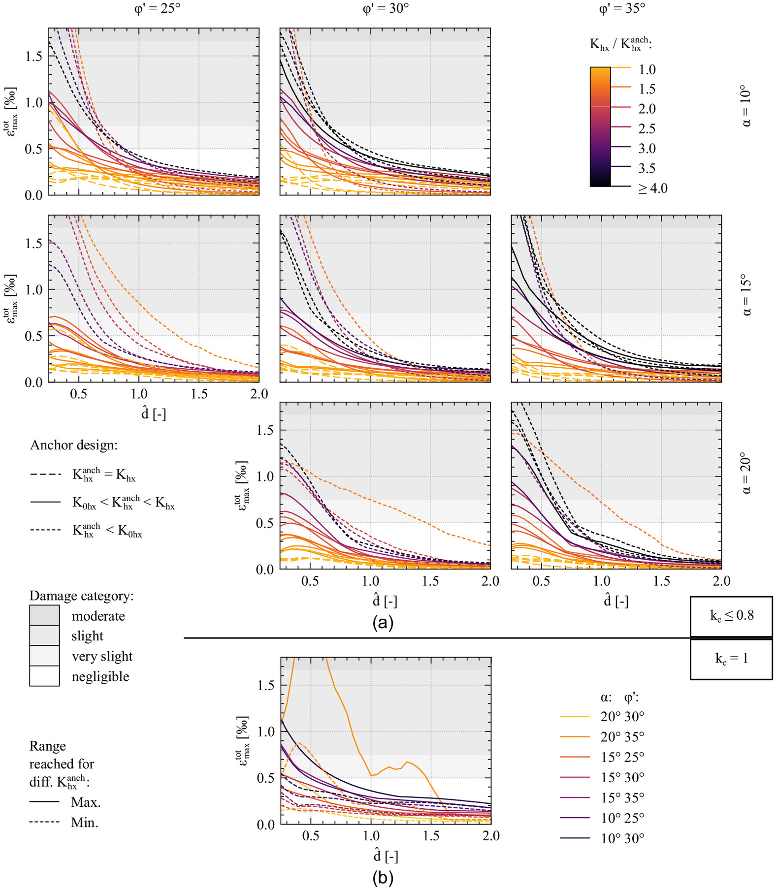
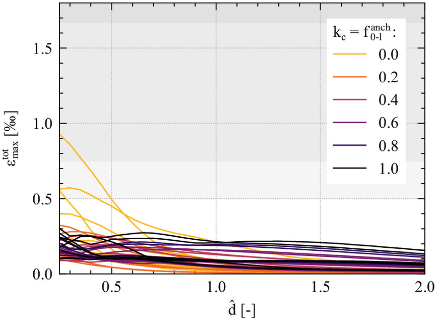
Fig. 20 shows the results of

ε_{\max}^{tot}

versus the normalized clear distance

\hat{d}

in the uphill sector. Models with

k_{c} < 1

and with

k_{c} = 1

are displayed separately. Unlike for the discussion of the downhill and the side sector,

k_{c}

is not a suitable indicator for the level of damage potential in the uphill sector. The level of anchorage

(K_{h x} / K_{h x}^{anch})

is introduced as an alternative parameter for the correlation to the damage potential:

1.

For the cases with

k_{c} < 1

and

K_{h x}^{anch} \geq K_{0 h x}

[Fig. 20(a), solid and dashed lines], within each pair of

α

and

φ^{'}

, the level of anchorage correlated well with the damage potential. The lower the level of anchorage, the higher was the damage potential. For low levels of anchorage, close neighbors must expect damage, whereas it can be avoided entirely for

K_{h x}^{anch} = K_{h x}

. Only for the cases with

K_{h x}^{anch} = K_{h x} = K_{0 h x}

(i.e.,

k_{c} = f_{0 - l}^{anch}

) did this correlation with the level of anchorage fail [Fig. 21, which displays all cases displayed with dashed lines in Fig. 20(a)]. However, the correlation can be re-established by assuming a triangular earth pressure distribution for the anchor design, as has been discussed regarding Fig. 8.

2.

Anchor design for increased active earth pressure, i.e.,

K_{h x}^{anch} < K_{0 h x}

[Fig. 20(a), dotted lines], generally led to higher damage than in any case with the same

α

and

φ^{'}

but

K_{h x}^{anch} \geq K_{0 h x}

, and thus the correlation with the level of anchorage does not hold here. For these cases, landslides and stable slopes (Fig. 10) had a roughly similar damage potential. An explanation for this high damage potential is most probably the large deformations accompanying plastic unloading when

K_{a h x} \leq K_{h x}^{anch} < K_{0 h x}

, in contrast to the mainly elastic deformation during unloading for

K_{h x}^{anch} \geq K_{0 h x}

.

3.

The cases with

k_{c} = 1

[Fig. 20(b)]; mostly did not fall particularly out of line, except the case with

α = 20 °

and

φ^{'} = 35 °

, which was treated in the discussion of the side sector.

Fig. 20. $ε_{\max}^{tot}$ versus $\hat{d}$ in the uphill sector for the landslide cases, with a distinction between different $φ^{'}$ and $α$ : (a) cases with $k_{c} \leq 0.8$ ; and (b) cases with $k_{c} = 1$ .

Fig. 21. $ε_{\max}^{tot}$ versus $\hat{d}$ in the uphill sector for all the landslide cases with $K_{h x}^{anch} = K_{h x}$ .

Conclusion

The five main outcomes of this study are summarized as follows:

•

When an excavation is being planned on sloping ground in an urban area, it is crucial to identify if the ground is stable or is moving as an active landslide, by carrying out a thorough site investigation beforehand. Furthermore, in case of a landslide, an accurate estimation of the compression state of the landslide at the site is very important. Failing to do so may lead to considerable damage to neighboring buildings, in particular in fully compressed landslides, in which a landslide failure wedge could form around the excavation.

•

For a proper anchor design, the limiting tensile strain method does not predict substantially higher damage potential for neighbors due to excavation in landslides than for stable slopes. A proper anchor design means that the anchors should be designed for the in situ earth pressure. However, for high landslide compression ratios this can lead to immense anchorage costs.

•

In addition to the generation of settlements and tensile strains, a distinctive and important feature of excavation within a landslide is the significant compressive strains that can develop in the sliding direction along the lateral sides of the excavation. A simplified analysis showed that these compressive strains also have the potential to damage neighboring buildings. This problem needs to be investigated in detail in future research.

•

The downhill sector, when constructed as an unsupported berm, remains practically unaffected by the anchor design on the side and uphill retaining walls. On the other hand, the deformations and the damage potential do increase for higher levels of landslide compression, potentially requiring a proper anchor support also on the downhill side of the excavation.

•

A key outcome of this study is the numerical modeling procedure, developed for the deformation and damage analysis. The most obvious measure to avoid damage to adjacent buildings when excavating in a landslide is simply to maintain sufficient distance. The proposed procedure not only allows for a quantification of safe distances from existing structures, but also provides input for the proper anchor design that would allow keeping damage within an acceptable range if the safe distance cannot be maintained.

Naturally, there are limitations to the extent, and therefore to the generality of the conducted parametric study. Such studies always are accompanied by modeling simplifications. One of the simplifications in this study lay in the modeling procedure of the excavation process. The excavation was carried out in one single stage, and the anchorage (modeled only as line loads) was introduced simultaneously. The influence of these simplifications is considered to be minor, because the results for stable slopes were validated against the literature in the “Results and Discussion” section. Moreover, the landslide results were always compared to these stable slope results, which readily allows for identification of good practices and areas in which a more detailed investigation or more research is required. Furthermore, due to the simplicity of the limiting tensile strain method, the results should be regarded as an estimation of the damage influence zone around a deep excavation, rather than providing accurate levels of damage for a specific case. If the geometrical or the material parameters in a specific case deviate significantly from those used in this study, it might be beneficial to model the case using the procedure described in this work. The procedure can be refined if a more accurate analysis is desired, e.g., modeling the excavation stages more precisely, or including an actual building at a specific location next to the excavation. Finally, the landslide was modeled in a simplified manner. Nevertheless, the key landslide characteristics were captured (i.e., possibility of movement along the shear zone, and presence of elevated or decreased earth pressure) by imposing the initial state and applying adequate boundary conditions. For cases in which the shear zone inclination differs greatly from the terrain inclination, especially for shallow landslides, the results of this work will not necessarily be applicable. The proposed procedure would have to be adapted accordingly in order to investigate such cases. Other than for such cases, the results produced and the conclusions are generally applicable, bearing in mind the aforementioned limitations. A final comment on the quality of the results of this study is that the ground deformations observed in the unpublished excavation cases in the Swiss town of St. Moritz were of the same order of magnitude as those predicted by the models proposed in this study.

Supplemental Materials

File (supplemental materials_jggefk.gteng-11318_hettelingh.pdf)

Download
706.97 KB

Data Availability Statement

Some or all data, models, or code that support the findings of this study are available from the corresponding author upon reasonable request, including the detailed formulation of soil material model, the detailed formulation of the contact law formulation for the shear zone, and the Abaqus user subroutine file.

Acknowledgments

Part of this research was funded by the Federal Office for the Environment (FOEN) of Switzerland.

References

Alonso, E. E., N. M. Pinyol, and A. M. Puzrin. 2010. “A constrained creeping landslide: Brattas-St. Moritz landslide, Switzerland.” In Geomechanics of failures. Advanced topics, 3–32. Dordrecht, Netherlands: Springer. https://doi.org/10.1007/978-90-481-3538-7_1.

Google Scholar

Angeli, M.-G., A. Pasuto, and S. Silvano. 1999. “Towards the definition of slope instability behaviour in the Alvera mudslide (Cortina d’Ampezzo, Italy).” Geomorphology 30 (1–2): 201–211. https://doi.org/10.1016/S0169-555X(99)00055-0.

Google Scholar

Béjar-Pizarro, M., et al. 2017. “Mapping vulnerable urban areas affected by slow-moving landslides using Sentinel-1 InSAR data.” Remote Sens. 9 (9): 876. https://doi.org/10.3390/rs9090876.

Google Scholar

Bonzanigo, L., E. Eberhardt, and S. Loew. 2007. “Long-term investigation of a deep-seated creeping landslide in crystalline rock. Part I. Geological and hydromechanical factors controlling the Campo Vallemaggia landslide.” Can. Geotech. J. 44 (10): 1157–1180. https://doi.org/10.1139/T07-043.

Google Scholar

Borrelli, L., G. Nicodemo, S. Ferlisi, D. Peduto, S. Di Nocera, and G. Gullà. 2018. “Geology, slow-moving landslides, and damages to buildings in the Verbicaro area (north-western Calabria region, southern Italy).” J. Maps 14 (2): 32–44. https://doi.org/10.1080/17445647.2018.1425164.

Google Scholar

Boscardin, M. D., and E. J. Cording. 1989. “Building response to excavation-induced settlement.” J. Geotech. Eng. 115 (1): 1–21. https://doi.org/10.1061/(ASCE)0733-9410(1989)115:1(1).

Google Scholar

Burland, J. B. 1995. “Assessment of risk of damage to buildings due to tunnelling and excavations.” In Vol. 3 of Proc., 1st Int. Conf. on Earthquake Geotechnical Engineering, IS-Tokyo’95, edited by K. Ishihara, 1189–1201. Rotterdam, Netherlands: A.A. Balkema.

Google Scholar

Burland, J. B., B. B. Broms, and V. F. B. De Mello. 1977. “Behaviour of foundations and structures.” In Proc., 9th Int. Conf. on Soil Mechanics and Foundation Engineering, 495–546. Tokyo: Japanese Society of Soil Mechanics and Foundation Engineering.

Google Scholar

Burland, J. B., and C. P. Wroth. 1974. “Settlement of buildings and associated damage.” In Proc., Settlement of Structures, edited by British Geotechnical Society, 611–654. London: Pentech Press.

Google Scholar

Caleca, F., V. Tofani, S. Segoni, F. Raspini, A. Rosi, M. Natali, F. Catani, and N. Casagli. 2022. “A methodological approach of QRA for slow-moving landslides at a regional scale.” Landslides 19 (7): 1539–1561. https://doi.org/10.1007/s10346-022-01875-x.

Google Scholar

Caquot, A., and J. Kérisel. 1948. Tables de butée, de poussée et de force portante des fondations. Paris: Gauthier-Villars.

Google Scholar

Caquot, A., and J. Kérisel. 1949. Traité de mécanique des sols. 2nd ed. Paris: Gauthier-Villars.

Google Scholar

Castaldo, R., P. Tizzani, P. Lollino, F. Calò, F. Ardizzone, R. Lanari, F. Guzzetti, and M. Manunta. 2015. “Landslide kinematical analysis through inverse numerical modelling and differential SAR interferometry.” Pure Appl. Geophys. 172 (11): 3067–3080. https://doi.org/10.1007/s00024-014-1008-3.

Google Scholar

CEN (European Committee for Standardization). 2004. Eurocode 7: Geotechnical design—Part 1: General rules. EN 1997-1. Brussels, Belgium: CEN.

Google Scholar

Cevasco, A., F. Termini, R. Valentino, C. Meisina, R. Bonì, M. Bordoni, G. P. Chella, and P. De Vita. 2018. “Residual mechanisms and kinematics of the relict Lemeglio coastal landslide (Liguria, northwestern Italy).” Geomorphology 320 (Nov): 64–81. https://doi.org/10.1016/j.geomorph.2018.08.010.

Google Scholar

Chen, Q., L. Chen, L. Gui, K. Yin, D. P. Shrestha, J. Du, and X. Cao. 2020. “Assessment of the physical vulnerability of buildings affected by slow-moving landslides.” Nat. Hazards Earth Syst. Sci. 20 (9): 2547–2565. https://doi.org/10.5194/nhess-20-2547-2020.

Google Scholar

Coulomb, C. A. 1776. “Essai sur une application des règles de maximis et minimis à quelques problemes de statique, relatifs à l’architecture.” In Mémoires de Mathématique et de Physique, Présentés à l’Académie Royale des Sciences, par divers Savans, & lûs dans les Assemblées. Année 1773, 343–382. Paris: L’Imprimerie Royale.

Google Scholar

Cruden, D. M. 1991. “A simple definition of a landslide.” Bull. Int. Assoc. Eng. Geol. 43 (1): 27–29. https://doi.org/10.1007/BF02590167.

Google Scholar

Cruden, D. M., and D. J. Varnes. 1996. “Landslide types and processes.” In Landslides: Investigation and mitigation, edited by A. K. Turner and R. L. Schuster, 36–75. Washington, DC: National Academy Press.

Google Scholar

Del Soldato, M., D. Di Martire, S. Bianchini, R. Tomás, P. De Vita, M. Ramondini, N. Casagli, and D. Calcaterra. 2019. “Assessment of landslide-induced damage to structures: The Agnone landslide case study (southern Italy).” Bull. Eng. Geol. Environ. 78 (4): 2387–2408. https://doi.org/10.1007/s10064-018-1303-9.

Google Scholar

Deutsche Gesellschaft für Geotechnik e.V. 2012. Empfehlungen des Arbeitskreises “Baugruben” (EAB). 5th ed. Berlin: Ernst & Sohn. https://doi.org/10.1002/9783433602478.

Google Scholar

Dille, A., et al. 2022. “Acceleration of a large deep-seated tropical landslide due to urbanization feedbacks.” Nat. Geosci. 15 (12): 1048–1055. https://doi.org/10.1038/s41561-022-01073-3.

Google Scholar

Ferlisi, S., A. Marchese, and D. Peduto. 2021. “Quantitative analysis of the risk to road networks exposed to slow-moving landslides: A case study in the Campania region (southern Italy).” Landslides 18 (1): 303–319. https://doi.org/10.1007/s10346-020-01482-8.

Google Scholar

Franke, E. 1974. ‘Ruhedruck in kohäsionslosen Böden.’ Accessed April 1, 2021. https://structurae.net/en/literature/journal-article/ruhedruck-in-kohasionslosen-boden.

Google Scholar

Friedli, B., D. Hauswirth, and A. M. Puzrin. 2017. “Lateral earth pressures in constrained landslides.” Géotechnique 67 (10): 1–16. https://doi.org/10.1680/jgeot.16.P.158.

Google Scholar

Guo, Z., L. Chen, K. Yin, D. P. Shrestha, and L. Zhang. 2020. “Quantitative risk assessment of slow-moving landslides from the viewpoint of decision-making: A case study of the Three Gorges Reservoir in China.” Eng. Geol. 273 (Aug): 105667. https://doi.org/10.1016/j.enggeo.2020.105667.

Google Scholar

Häusler, M., V. Gischig, R. Thöny, F. Glueer, and F. Donat. 2021. “Monitoring the changing seismic site response of a fast-moving rockslide (Brienz/Brinzauls, Switzerland).” Geophys. J. Int. 229 (1): 299–310. https://doi.org/10.1093/gji/ggab473.

Google Scholar

Infante, D., D. Di Martire, P. Confuorto, M. Ramondini, D. Calcaterra, R. Tomás, J. Duro, and G. Centolanza. 2017. “Multi-temporal assessment of building damage on a landslide-affected area by interferometric data.” In Proc., 3rd Int. Forum on Research and Technologies for Society and Industry (RTSI). New York: IEEE. https://doi.org/10.1109/RTSI.2017.8065907.

Google Scholar

Kohler, M., and A. M. Puzrin. 2022. “Mechanism of co-seismic deformation of the slow-moving La Sorbella landslide in Italy revealed by MPM analysis.” J. Geophys. Res.: Earth Surf. 127 (7): e2022JF006618. https://doi.org/10.1029/2022JF006618.

Google Scholar

Kondner, R. L., and J. S. Zelasko. 1963. “A hyperbolic stress-strain formulation of sands.” In Vol. 1 of Proc., 2nd Pan American Conf. on Soil Mechanics and Foundation Engineering, 289–324. Sao Paulo, Brazil: Associacao Brasileira de Mecanica dos Solos.

Google Scholar

Lu, P., F. Catani, V. Tofani, and N. Casagli. 2014. “Quantitative hazard and risk assessment for slow-moving landslides from Persistent Scatterer Interferometry.” Landslides 11 (4): 685–696. https://doi.org/10.1007/s10346-013-0432-2.

Google Scholar

Mansour, M. F., N. R. Morgenstern, and C. D. Martin. 2011. “Expected damage from displacement of slow-moving slides.” Landslides 8 (1): 117–131. https://doi.org/10.1007/s10346-010-0227-7.

Google Scholar

Nappo, N., O. Mavrouli, F. Nex, C. J. van Westen, R. Gambillara, and A. M. Michetti. 2021. “Use of UAV-based photogrammetry products for semi-automatic detection and classification of asphalt road damage in landslide-affected areas.” Eng. Geol. 294 (Dec): 106363. https://doi.org/10.1016/j.enggeo.2021.106363.

Google Scholar

Nappo, N., D. Peduto, O. Mavrouli, C. J. van Westen, and G. Gullà. 2019. “Slow-moving landslides interacting with the road network: Analysis of damage using ancillary data, in situ surveys and multi-source monitoring data.” Eng. Geol. 260 (Oct): 105244. https://doi.org/10.1016/j.enggeo.2019.105244.

Google Scholar

Netzel, H. 2005. “Review of the limiting tensile strain method for predicting settlement induced building damage.” In Proc., Geotechnical Aspects of Underground Construction in Soft Ground: Proc. of the 5th Int. Symp. TC28, edited by K. J. Bakker, A. Bezuijen, W. Broere, and E. A. Kwast, 159–164. Boca Raton, FL: CRC Press.

Google Scholar

Notti, D., J. P. Galve, R. M. Mateos, O. Monserrat, F. Lamas-Fernández, F. Fernández-Chacón, F. J. Roldán-García, J. V. Pérez-Peña, M. Crosetto, and J. M. Azañón. 2015. “Human-induced coastal landslide reactivation. Monitoring by PSInSAR techniques and urban damage survey (SE Spain).” Landslides 12 (5): 1007–1014. https://doi.org/10.1007/s10346-015-0612-3.

Google Scholar

Oberender, P. W., and A. M. Puzrin. 2016. “Observation-guided constitutive modelling for creeping landslides.” Géotechnique 66 (3): 232–247. https://doi.org/10.1680/jgeot.15.LM.003.

Google Scholar

Oberender, P. W., D. V. Val, and A. M. Puzrin. 2020. “Mechanical models for hazard and risk analysis of structures in creeping landslides.” Geotech. Eng. 51 (3): 52–59.

Google Scholar

Peck, R. B. 1969. “Deep excavations and tunneling in soft ground.” In Proc., 7th Int. Conf. on Soil Mechanics and Foundation Engineering, 225–290. Mexico City: Sociedad Mexicana de Mecanica de Suelos.

Google Scholar

Peduto, D., S. Ferlisi, G. Nicodemo, D. Reale, G. Pisciotta, and G. Gullà. 2017. “Empirical fragility and vulnerability curves for buildings exposed to slow-moving landslides at medium and large scales.” Landslides 14 (6): 1993–2007. https://doi.org/10.1007/s10346-017-0826-7.

Google Scholar

Peduto, D., G. Nicodemo, M. Caraffa, and G. Gullà. 2018. “Quantitative analysis of consequences to masonry buildings interacting with slow-moving landslide mechanisms: A case study.” Landslides 15 (10): 2017–2030. https://doi.org/10.1007/s10346-018-1014-0.

Google Scholar

Polshin, D. E., and R. A. Tokar. 1957. “Maximum allowable non-uniform settlement of structures.” In Proc., 4th Int. Conf. on Soil Mechanics and Foundation Engineering, 402–405. London: Butterworths Scientific.

Google Scholar

Puzrin, A. M., and A. M. Schmid. 2011. “Progressive failure of a constrained creeping landslide.” Proc. R. Soc. A 467 (2133): 2444–2461. https://doi.org/10.1098/rspa.2011.0063.

Google Scholar

Puzrin, A. M., and A. M. Schmid. 2012. “Evolution of stabilised creeping landslides.” Géotechnique 62 (6): 491–501. https://doi.org/10.1680/geot.11.P.041.

Google Scholar

Rowe, P. W. 1962. “The stress-dilatancy relation for static equilibrium of an assembly of particles in contact.” Proc. R. Soc. London, Ser. A 269 (1339): 500–527. https://doi.org/10.1098/rspa.1962.0193.

Google Scholar

Rowe, P. W. 1971. “Theoretical meaning and observed values of deformation parameters for soil.” In Proc., Stress-Strain Behaviour of Soils: Proc. of the Roscoe Memorial Symp., edited by R. H. G. Parry and K. H. Roscoe, 143–194. Henley-on-Thames, UK: G. T. Foulis.

Google Scholar

Schanz, T., and P. A. Vermeer. 1996. “Angles of friction and dilatancy of sand.” Géotechnique 46 (1): 145–151. https://doi.org/10.1680/geot.1996.46.1.145.

Google Scholar

Schanz, T., and P. A. Vermeer. 1998. “On the stiffness of sands.” In Pre-failure deformation behaviour of geomaterials, 383–387. London: Thomas Telford.

Google Scholar

Schanz, T., P. A. Vermeer, and P. G. Bonnier. 1999. “The hardening soil model: Formulation and verification.” In Proc., Beyond 2000 in Computational Geotechnics. Ten Years of PLAXIS Int. Proc. of the Int. Symp., edited by R. B. J. Brinkgreve, 281–296. Rotterdam, Netherlands: A.A. Balkema. https://doi.org/10.1201/9781315138206-27.

Google Scholar

SIA (Schweizerischer Ingenieur- und Architektenverein). 2020. Einwirkungen auf Tragwerke. SIA 261. SN 505 261. Zurich, Switzerland: SIA.

Google Scholar

Skempton, A. W., and D. H. MacDonald. 1956. “The allowable settlements of buildings.” Proc. Inst. Civ. Eng. 5 (6): 727–768. https://doi.org/10.1680/ipeds.1956.12202.

Google Scholar

Son, M., and E. J. Cording. 2005. “Estimation of building damage due to excavation-induced ground movements.” J. Geotech. Geoenviron. Eng. 131 (2): 162–177. https://doi.org/10.1061/(ASCE)1090-0241(2005)131:2(162).

Google Scholar

Tacher, L., C. Bonnard, L. Laloui, and A. Parriaux. 2005. “Modelling the behaviour of a large landslide with respect to hydrogeological and geomechanical parameter heterogeneity.” Landslides 2 (1): 3–14. https://doi.org/10.1007/s10346-004-0038-9.

Google Scholar

Terzaghi, K. 1941. “General wedge theory of earth pressure.” Trans. Am. Soc. Civ. En. 106 (1): 68–80. https://doi.org/10.1061/TACEAT.0005429.

Google Scholar

Uzielli, M., F. Catani, V. Tofani, and N. Casagli. 2015. “Risk analysis for the Ancona landslide—II: Estimation of risk to buildings.” Landslides 12 (1): 83–100. https://doi.org/10.1007/s10346-014-0477-x.

Google Scholar

von Soos, P., and J. Bohac. 2002. “Properties of soils and rocks and their laboratory determination.” In Geotechnical engineering handbook, Volume 1: Fundamentals, edited by U. Smoltczyk, 116–206. Berlin: Ernst und Sohn.

Google Scholar

Information & Authors

Information

Published In

Journal of Geotechnical and Geoenvironmental Engineering

Volume 149 • Issue 9 • September 2023

Copyright

This work is made available under the terms of the Creative Commons Attribution 4.0 International license, https://creativecommons.org/licenses/by/4.0/.

History

Received: Sep 8, 2022

Accepted: Apr 4, 2023

Published online: Jul 11, 2023

Published in print: Sep 1, 2023

Discussion open until: Dec 11, 2023

Authors

Affiliations

Roman Hettelingh https://orcid.org/0000-0002-3119-5619 [email protected]

Doctoral Student, Institute for Geotechnical Engineering, ETH Zurich, Zurich 8093, Switzerland (corresponding author). ORCID: https://orcid.org/0000-0002-3119-5619. Email: [email protected]

View all articles by this author

Alexander M. Puzrin, Ph.D. https://orcid.org/0000-0002-9566-8841

Professor, Institute for Geotechnical Engineering, ETH Zurich, Zurich 8093, Switzerland. ORCID: https://orcid.org/0000-0002-9566-8841

View all articles by this author

Metrics & Citations

Metrics

Citations

Download citation

If you have the appropriate software installed, you can download article citation data to the citation manager of your choice. Simply select your manager software from the list below and click Download.

Abstract

Introduction

Modeling

Model Geometry

Landslide

Excavation Pit

Constitutive Laws and Material Properties

Sliding Soil Mass

Shear Zone

Excavated Soil Mass, Retaining Walls, and Soil Anchors

Boundary and Initial Conditions

Initial Stress State

Static and Kinematic Boundary Conditions on the Landslide

Anchor Prestressing Forces

FE Model Progression

Postprocessing of the Results

Layout of the Parametric Study

Results and Discussion

Stable Slopes

Comparison of Stable Slopes and Landslides

Compressed Landslides

Downhill Sector

Side Sectors

Uphill Sector

Conclusion

Supplemental Materials

Data Availability Statement

Acknowledgments

References

Information

Published In

Copyright

History

Authors

Affiliations

Metrics

Citations

Download citation

Figures

Other

Share

Copy the content Link

Share with email

Share

Request Username

Create a new account

Change Password

Password Changed Successfully

Verify Phone

Congrats!