Macromechanism Approach for Vulnerability Assessment of Buildings on Shallow Foundations in Liquefied Soils

Viana da Fonseca, Antonio; Millen, Maxim; Quintero, Julieth; Sargin, Sinan; Rios, Sara; Romão, Xavier; Pereira, Nuno; Panico, Fabrizio; Oztoprak, Sadik; Kelesoglu, M. Kubilay

doi:10.1061/JGGEFK.GTENG-10881

Open access

Technical Papers

Jan 10, 2023

Macromechanism Approach for Vulnerability Assessment of Buildings on Shallow Foundations in Liquefied Soils

Publication: Journal of Geotechnical and Geoenvironmental Engineering

Volume 149, Issue 3

https://doi.org/10.1061/JGGEFK.GTENG-10881

PDF

Abstract

The damage caused by seismic shaking and liquefaction-induced permanent ground deformation has conventionally been assessed as two separate problems often by different engineers. However, the two problems are inherently linked, since ground shaking causes liquefaction, and liquefaction-induced soil softening affects ground shaking. Modelling both problems within a single numerical model is complex for both the engineer and the software, and most finite element software only have the capabilities to address one of them. To improve the estimates of the seismic performance of buildings on liquefiable soil, a new sub-structuring approach is proposed called the macro-mechanism approach. This approach allows the soil-liquefaction-foundation-structure interaction to be considered in a series of sub-models accounting for the major nonlinear mechanisms of the system at a macro level. The proposed approach was implemented in the open-source finite element software OpenSees and then applied to a case study of a building where significant liquefaction- and shaking-induced damage was observed after the 1999 Mw 7.4 Kocaeli Earthquake. The case study building was also simulated using two different commercial software programs, the finite difference software FLAC, and the finite element software PLAXIS, by two different research teams. A comparison between the results from the macro-mechanism approach compared to full numerical models shows that the macro-mechanism approach can capture the extent of the foundation deformation and provide more realistic estimates of the building damage than full approaches since the FLAC and PLAXIS models consider elastic elements for the building.

Introduction

Vulnerability assessments of buildings on shallow foundations in liquefiable soils have been mainly focused on soil deformation and the consequent damage to foundations. Since soil softening associated with liquefaction acts as a natural isolation barrier (Karatzia et al. 2019), the damage associated with strong ground shaking, in conjunction with ground deformation, is often neglected. However, several studies (Dashti et al. 2010; Kramer et al. 2011) have demonstrated that when liquefaction occurs later in the strong shaking, buildings can experience both significant settlement and strong shaking. In fact, partial liquefaction under a building leads to soil deformation and consequent changes in its dynamic properties, which can then potentially amplify its dynamic response. To better understand strong shaking-induced damage when liquefaction occurs, the interactions between the soil, foundation, and structure must be well defined, and a framework should be established to account for the combined damage and loss induced by both soil-foundation deformation and shaking (Millen et al. 2018).

While there are efforts to quantify the vulnerability of buildings to liquefaction using empirical field data sets (Paolella et al. 2020), these approaches are limited by the availability and quality of the data. Three alternative analytical approaches have been identified and adopted to consider soil-liquefaction-foundation-structure interaction (SLFSI) in building vulnerability (Fig. 1). The building-soil system can be assessed directly by modelling both soil and building in a single numerical or experimental model (a full model approach), such as in Dashti and Bray (2013), and Ramirez et al. (2018). Alternatively, the building response and soil response can be completely decoupled. In this case, shaking and liquefaction damage are assessed independently and then combined through an interaction function (separate hazards approach), such as in the HAZUS methodology (FEMA 2003), the proposal by Bird et al. (2006), or imposing ground deformations directly or indirectly to a building (Fotopoulou et al. 2018; Gómez-Martinez et al. 2020).

Fig. 1. Different modelling approaches for soil-liquefaction-foundation-structure-interaction.

The full model approach, where both soil and structure are modelled together with adequate constitutive laws in a single simulation, is advantageous because the interactions between all mechanisms are accounted for implicitly. However, it is a demanding task to develop an adequate full model that accurately captures the complex effective stress-controlled soil behavior and the various nonlinear mechanisms in a building. Notably, none of the widely used commercial software currently contain both a three-dimensional state-compatible constitutive model for the soil, and elements for modelling existing structures (e.g., reinforced concrete buildings) with a suitable array of nonlinear material constitutive models. Therefore, a trade-off must be made by reducing the accuracy for the soil or the structural modelling. In addition, the full model approach is computationally demanding as nonlinear structural models with degrading behavior often require very small time steps to achieve convergence, but in a large soil domain medium, there are many degrees of freedom that must be assessed at each time step.

The separate hazards approach is numerically efficient and can make use of existing results for ground shaking damage (e.g., fragility functions), but it suffers from some significant drawbacks. The use of an interaction function to combine shaking and liquefaction damage is non-trivial as will be shown in the next section. Essentially, liquefaction modifies the shaking demand, and differential settlements affect the lateral resistance capacity of the building, which influences the shaking damage. Meanwhile, liquefaction-induced settlement and tilt are dependent on the inertial load (shaking) of the building.

In this article, an innovative modular approach is proposed for reinforced concrete-framed structures on shallow foundations in liquefiable soil deposits, where different macro-mechanisms are first quantified and then connected based on their interactions. The idea is to capture the full system behavior through a combination of sub-models (e.g., a pore pressure model, a settlement model) that focus on a particular mechanism or system behavior, rather than at the constitutive level. For this reason, it has been termed the macro-mechanism approach. The procedure presented here has been applied in an extensive parametric study described in Viana da Fonseca et al. (2018) for the development of the fragility functions for the loss assessment LIQUEFACT software (Meslem et al. 2019), and to assess liquefaction-induced loss at critical infrastructure as described by Meslem et al. (2021).

In this work, the approach is described in detail and then a validation study is performed focusing on the behavior of the Public Education Center (PEC) building in Adapazari, Turkey, during the 1999 Kocaeli earthquake. As part of the validation study, the PEC building is modelled using the macro-mechanism approach in OpenSees, as well as using two full numerical models in FLAC (version 8.0) (Itasca 2016) and PLAXIS (Bentley 2020) that were developed by separate research teams at the University of Porto and Istanbul University-Cerrahpasa, respectively, to allow for comparisons between the performances of the different models.

The Macro-Mechanism Approach

Methodology Description

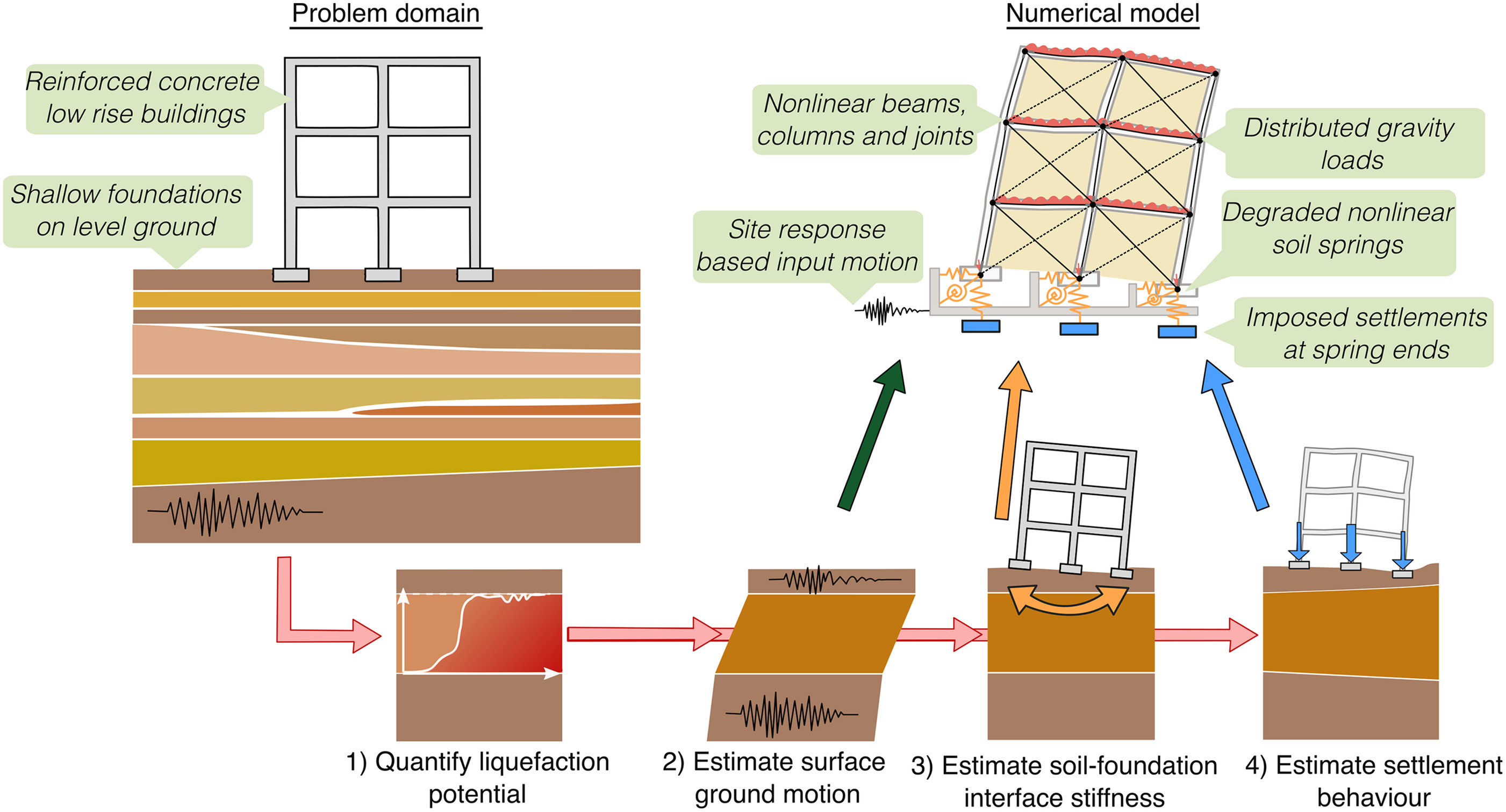
A nonlinear time history analysis procedure that models the macro-mechanisms of the soil, foundation, and structure during a shaking event has been developed. This procedure is a sub-structuring approach and has been developed to provide an efficient method to consider the impact of liquefaction on the performance of buildings. The problem domain of the proposed procedure is reinforced concrete buildings founded on shallow foundations on flat ground, and subjected to a ground motion applied only in one principal direction of the building. The so-called macro-mechanism approach addresses the three liquefaction-induced macro-mechanisms of changes in ground shaking, changes in foundation impedances, and settlement, through a series of time-dependent sub-models that are subsequently integrated into a time history analysis of the building using springs, dashpots, and imposed displacements. The development of the model requires four steps that can be performed separately or in combination:

1.

Quantify the liquefaction potential of the soil profile in terms of depth and thickness of the liquefiable layer(s) and the resistance to liquefaction. The free-field pore pressure ratio is then quantified throughout the duration of shaking.

2.

Estimate the near-field ground shaking time series accounting for liquefaction for use as acceleration input for the building time history analysis.

3.

Estimate the soil-foundation stiffness using springs and dashpots and account for the change in soil characteristics due to liquefaction and nonlinear shear deformation throughout the duration of shaking.

4.

Estimate the expected load-settlement behavior of each footing accounting for the expected level of pore pressure build up throughout the duration of shaking.

The key aspects of this approach can be seen in Fig. 2, where the outputs of the four steps are used as inputs into a nonlinear model of the building. The input motion is the expected near-field motion from Step 2 and the expected differential settlement behavior is captured through a combination of imposed settlement (Step 4) and changes in the stiffness of the soil springs (Step 3). In this paper, a procedure for completing each sequential step is presented. It is recognized that this decoupling introduces inaccuracies, and in the case study, an additional analysis is performed where ground shaking, pore pressure, and settlement are obtained from a fully-coupled 2D FLAC analysis to demonstrate the flexibility of the macro-mechanism approach.

Estimation of Excess Pore Pressure

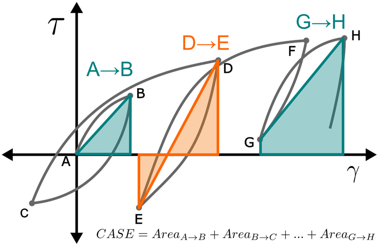
The build up of excess pore pressure in free-field conditions can be either estimated through a 1D effective stress analysis, or through simplified pore pressure models. There are several simplified pore pressure models to estimate liquefaction that are often separated into stress-based, strain-based, or energy-based. Some of them only provide the factor of safety against liquefaction triggering, but others provide the whole pore pressure evolution during the earthquake duration including the time of liquefaction triggering. In this work, the strain energy-based model proposed by Millen et al. (2020) was used, but other simplified models that provide the pore pressure time series could be used instead (see Seed et al. 1975; Green et al. 2000; Kokusho 2013; Rios et al. 2019). In the method developed by Millen et al. (2020), liquefaction resistance is measured in terms of normalized cumulative absolute strain energy (NCASE), which was shown to be insensitive to loading amplitude but sensitive to soil properties. NCASE is defined as the cumulative change in absolute elastic strain energy divided by the initial vertical effective stress,

σ_{v o}^{'}

, [Eqs. (1) and (2) and Fig. 3] which can be determined directly from laboratory testing, or a semi-analytical correlation (see Millen et al. 2020), where

τ

is the shear stress and

γ

is the shear strain

N C A S E = \frac{1}{σ_{v 0}^{'}} \sum_{j = 0}^{n_{p e a k s}} | τ_{a v., j} | \cdot | γ_{j + 1} - γ_{j} |

(1)

τ_{a v ., j} = {\begin{matrix} \frac{| τ_{j + 1} + τ_{j} |}{2} & τ_{j + 1} \cdot τ_{j} \geq 0 \\ \frac{| τ_{j + 1}^{2} + τ_{j}^{2} |}{2 \cdot | τ_{j + 1} - τ_{j} |} & τ_{j + 1} \cdot τ_{j} < 0 \end{matrix}}

(2)

Fig. 3. Graphical calculation of cumulative absolute strain energy.

The estimated NCASE demand can be obtained using the nodal surface energy spectrum (NSES), which provides an exact solution for the NCASE at any depth in a homogeneous purely linear elastic soil deposit, and additional correction factors have been proposed by Millen et al. (2020) to account for soil nonlinearity and heterogeneous soil profiles. The NSES method takes the upward motion and combines it with an approximate downward wave (itself but with a depth-dependent time shift that corresponds to the time taken for the seismic wave to travel from the depth of interest to the surface and back). The upward and downward waves are subtracted and the cumulative absolute change in kinetic energy of this combined motion is computed, which corresponds to the NCASE at the depth of interest. This procedure has been implemented into the open-source Python package Liquepy (Millen and Quintero 2022) (see Millen et al. 2020; Rios et al. 2022, for details).

Estimation of Surface Ground Motion

In terms of the dynamic response of soil deposits, the soil profile acts as a filter and converts the upward propagating wave to a surface motion. This step can be achieved through effective stress modelling, either of a one-dimensional soil column or a multi-dimensional half space, or through simplified models that account for the change in dynamic behavior due to liquefaction. In this work, the Equivalent Linear Stockwell Analysis (ELSA) method, initially proposed in Viana da Fonseca et al. (2018) and extended by Millen et al. (2021), is used for this purpose. The method makes use of the Stockwell transform to apply time-dependent equivalent linear transfer functions to the input motion to simulate the site response of a liquefying deposit. In the ELSA method, the pore pressure in the free-field is used as there is currently no suitable method to directly estimate excess pore pressure under a building.

The method from Millen et al. (2021) consists of the eight steps below, as implemented in the Liquepy Python package (Millen and Quintero 2022)

1.

Define modulus reduction and damping curves for each layer of soil (Darendeli 2001).

2.

Perform an equivalent linear analysis and obtain the strain time series in each layer. In this study, the analysis was performed using the open-source Python package PySRA v0.3.0 (Kottke 2018).

3.

Adjust the modulus reduction and damping values based on the time series for each layer, where each strain time series is split into one-second intervals and the peak shear strain is taken as the maximum value from a three-second window centered around each one-second interval. The effective strain for each segment is then taken as 90% of the peak strain.

4.

Estimate the excess pore pressure ratio time series in each liquefiable layer, using available methods [the method from Millen et al. (2020) outlined in the section above was used in this study].

5.

Using the pore pressure (Step 4) and the strain (Step 3), calculate a pore pressure-adjusted shear modulus and damping in each layer for each time interval using equations from Millen et al. (2021).

6.

Develop transfer functions for each time interval that convert the input motion to the surface acceleration.

7.

Compute the Stockwell transform of the input motion.

8.

Apply each transfer function to the input Stockwell transform at the appropriate time interval to produce the surface Stockwell transform.

9.

Invert the surface Stockwell transform to obtain the surface acceleration time series.

Estimation of Soil-Foundation Interface Stiffness

Soil-foundation impedance was modelled using the procedure outlined in Millen et al. (2019) where a single spring and dashpot were used for each vertical, horizontal, and rotational degree of freedom of each footing. The initial spring and dashpot properties were determined using the formulations proposed in Gazetas (1991). The horizontal stiffness was modelled as constant linear elastic, while the vertical and rotational springs were degraded based on the change in excess pore pressure ratio,

r_{u}

(where

r_{u}

is defined as the excess pore water pressure divided by the initial vertical effective stress).

The vertical stiffness was modelled as a linear no-tension spring. However, the spring stiffness decreased linearly with an increase in

r_{u}

from an initial value

K_{v; I}

, corresponding to

r_{u} = 0

, to a residual value

K_{v; res}

at

r_{u} = 1

, where the residual value was calculated based on Karatzia et al. (2017) and a shear wave velocity for the liquefied soil of

30 m / s

[15% of the initial value consistent with the range of 10%–30% provided by Karatzia et al. (2017)]. The stiffness was calculated at each step by reading the

r_{u}

time series from the center of the liquefiable layer in the free-field. Original research by Karatzia et al. (2017) assumed that the liquefiable layer had the same properties under the building as in the free-field, and this assumption is also made here and may under- or over-estimate the soil stiffness, as the presence of the building modifies pore pressure build up and confining stress. The change in the vertical stiffness was not intended to capture the liquefaction-induced settlement (which was modelled through vertical displacements at the spring ends and is typically driven by several mechanisms as well as vertical loading) as the spring deformation in the case study below was less than 2 mm. However, the vertical resistance of the soil can be a crucial parameter in the redistribution of loads and in the change of the dynamic response period of the soil-foundation-structure system. The macro-mechanism structural model was developed in OpenSees and the vertical spring was modelled using the elastic no-tension material (ENT material), which allowed for regular updating of the stiffness.

The rotational spring was both deformation- and pore pressure-dependent and was modelled in OpenSees using the uniaxial p-y material PyLiq1 (Boulanger et al. 1999) that allows the stiffness and strength to decrease due to a pore pressure time series and can represent the rocking behavior of a foundation. Herein, the ultimate moment capacity was the input for the non-liquefied soil calculated using

M_{c a p, i} = M_{y} = N \frac{B}{2} (1 - \frac{N}{N_{c a p}})

(3)

where

B

is the footing width,

N

is the static vertical load, and

N_{c a p}

is the foundation bearing capacity in static conditions. To estimate the residual moment capacity, required for the PyLiq1 material, the non-liquefied moment capacity was reduced down by a factor equal to the ratio of liquefied to non-liquefied rotational stiffness from Karatzia et al. (2017). The free-field pore pressure time series was inputted directly into the PyLiq1 material to reduce both the stiffness and capacity. The rotational damping was modelled within the PyLiq1 element, whereas the damping for the other modes was modelled with dashpot elements in parallel with the springs.

Estimation of Settlements

There are several methods available for the simplified assessment of foundation settlement on liquefied soil (Bray and Macedo 2017; Bullock et al. 2019b; Karamitros et al. 2013). Due to the modular nature of the macro-mechanism approach, all procedures can be applied to quantify epistemic uncertainty. The validation study presented in the next section uses the following equation proposed by Bray and Macedo (2017), which was developed from a best-fit regression using the results of a numerical two-dimensional parametric analysis

\ln (D_{S}) = c_{1} + 4.59 \cdot \ln (Q) - 0.42 \cdot \ln {(Q)}^{2} + c_{2} \cdot L B S + 0.58 \cdot \ln (\tanh (H_{L})) - 0.02 \cdot B + 0.84 \cdot \ln (C A V d p) + 0.41 \cdot \ln (S_{a}) + ε

(4)

where

D_{S}

is the foundation settlement, constants

c_{1}

and

c_{2}

depend on the liquefaction-induced building settlement index (LBS) defined by Eq. (5 ) and have values of

- 8.35

and 0.072, respectively, for

LBS < 16

, and

- 7.48

and 0.014 otherwise. Q is the foundation contact pressure,

H_{L}

is the liquefiable layer thickness, B is the building width,

S_{a}

is the spectral acceleration at a period equal to 1 s, and

ε

is a normal random variable with zero mean and a standard deviation of 0.50.

The LBS index, as defined in Eq. (5), is a weighted liquefaction-induced shear strain in the free-field. The value of the free-field shear strain,

ε_{shear}

, is calculated using Zhang et al. (2004), based on the estimated relative density (

D_{r}

) of the liquefied soil layer and the calculated safety factor against liquefaction triggering (FSL). Parameter z (m) in Eq. (5) is the depth measured from the ground surface (

> 0

) and W is a foundation-weighting factor wherein W is 0.0 for z values less than

D_{f}

, which is the embedment depth of the foundation, and 1.0 otherwise.

To determine the standardized Cumulate Absolute Velocity (CAVdp) as defined in Campbell and Bozorgnia (2012), Eq. (6) was used, where N is the number of discrete one-second time intervals and H(x) is 0 if

x < 0

or 1 otherwise. x is (

{PGA}_{i} - 0.025

) where

{PGA}_{i}

is the value of the peak ground acceleration (in g) in each one-second time interval i, inclusive of the first and last values

L B S = \int W \cdot \frac{ε_{s h e a r}}{z} d z

(5)

C A V d p = \sum_{i = 1}^{N} (H (x) \int_{i - 1}^{i} | a (t) | d t)

(6)

To convert the settlement value from Eq. (4) to a time series, either CAVdp can be used as a time series, with all other values as scalars, or additionally the LBS can be considered a time series where the

ε_{s h e a r}

parameter is computed for a time-dependent factor of safety that can be determined using the acceleration time series and a cycle counting procedure or based on the free-field pore pressure time series. The latter option results in less settlement in the initial portion of shaking but ultimately obtains a similar value if the final

ε_{s h e a r}

is similar to the scalar value. For the validation study in Adapazari, Eq. (4) was used with only CAVdp as a time series to estimate the settlements for the five footings of the building using each footing load and width. Then, an average settlement time series of all five footings was calculated to be used in the central footing, with other footings adjusted by the expected tilt.

The settlement of each footing (except the central footing) was estimated by multiplying the average settlement pre-calculated using the Bray and Macedo (2017) method (S) by a constant coefficient based on the expected level of tilt (

θ

). The estimation of this coefficient is based on the simplified empirical model (Bullock et al. 2019a), which results in Eq. (7) below

c o e f f = [\frac{S + x_{f o o t} \cdot \tan θ}{S}]

(7)

where

x_{foot}

is the distance from each footing axis to the middle of the structure and

θ

is the global tilt.

The Simplified Empirical Model for Residual Tilt (Bullock et al. 2019a) can be used to estimate the global tilt. Since this model is based entirely on case histories, it does not suffer from a simulation introduced bias. However, Bullock et al. (2019a) identified that direct numerical simulations resulted in general underprediction in tilt, and stated as potential causes, that the numerical models did not fully incorporate the 3D heterogeneity and ejecta observed in the field. The adopted Bullock et al. (2019a) model depends only on the width of the mat foundation (B, being in this case the total width of the structure), the thickness of the non-liquefiable crust (

D_{S, T}

), and the average settlement experienced by the foundation (S), as shown in Eq. (8)

\ln {(θ)}_{r} = a_{1} \cdot \ln (S) + a_{2} \cdot \ln (B) + a_{3} \cdot D_{S, T} + ε_{r^{e}}

(8)

where

a_{1} = 0.509

,

a_{2} = - 0.936

and

a_{3} = - 0.102

are fitted parameters and

ε_{r^{e}}

is an error term that follows a normal distribution with zero mean and a standard deviation of 0.29.

The global tilt (

θ

) used in Eq. (7) is a probabilistic value calculated using

θ = {(θ)}_{r} \pm σ_{r^{e}}^{*}

(9)

where

σ_{r^{e}}^{*}

represents the total uncertainty (Bullock et al. 2019a) expressed in Eq. (10)

σ_{r^{e} =}^{*} {\begin{cases} σ_{r^{e}, 1} & B \leq B_{1}^{*} \\ σ_{r^{e}, 1} - (σ_{r^{e}, 1} - σ_{r^{e}, 2}) \frac{(B - B_{1}^{*})}{(B_{2}^{*} - B_{1}^{*})} & B_{1}^{*} < B \leq B_{2}^{*} \\ σ_{r^{e}, 2} & B_{2}^{*} < B \end{cases}

(10)

where

B_{1}^{*}

and

B_{2}^{*}

are threshold values of B that correspond to the values for which heteroscedasticity is observed. The parameter values suggested by Bullock et al. (2019a) are

a_{1} = 0.509

,

a_{2} = - 0.936

,

a_{3} = - 0.102

,

σ_{r^{e}} = 0.287

,

B_{1}^{*} = 12

,

B_{2}^{*} = 16

,

σ_{r^{e}, 1} = 0.342

, and

σ_{r^{e}, 2} = 0.123

.

The footing settlement is applied to the soil end of the soil springs, whereas the actual settlement differs due to load redistribution, and variations in spring stiffness and footing load. The application of displacements to the soil end is preferred, compared to direct application of differential settlements where loads and displacements do not account for the structural stiffness and can be unrealistic (Gómez-Martinez et al. 2020).

System Validation: Application to a Case Study in Adapazari

Description of the Case Study

To demonstrate the applicability and validity of the macro-mechanism approach, a building from Adapazari, Turkey, was simulated. To understand the efficacy of the approach, the building was also simulated using two full numerical models, using two different software packages managed by different research teams. Adapazari is the capital of Sakarya City in Turkey, which was significantly affected by the large Kocaeli earthquake of August 17, 1999, where widespread foundation damage occurred. Post-earthquake reconnaissance surveys showed that most of the buildings that suffered from ground failures were buildings with shallow raft foundations. Several of these cases were investigated in great detail by various researchers (Bay and Cox 2001; Yoshida et al. 2001; Sancio 2003; UC Berkeley et al. 2003). One of these damaged buildings was the PEC building of Adapazari, and it differed from the other cases due to its foundation type; this building was built with isolated footings. The presence of isolated footings changed the mechanisms of the damage pattern of the structure and the footings due to differential settlements.

Fig. 4 shows photographs of the PEC building about 10 days after the earthquake. This case was presented in the Earthquake Engineering Online Archive of the NISEE e-Library by Prof. Halil Sezen and Prof. Kenneth J. Elwood (NISEE 2022). Prof. Sezen and Prof. Elwood described the damage in the PEC building as:

“Rotation at the base of the shear wall and settlement of the footings beneath the moment-frame columns contributed to the failure of ground floor columns. The column in the middle axis failed under shear and axial loads. Note that the columns on the sides discontinued. Settlement of footings beneath the moment-frame columns contributed to failure of ground floor columns.”

and as:

“Damage to beams and columns. No cracks were observed in the shear wall, but the right end of the wall settled approximately 20 inches due to bearing failure of supporting soils. Damaged wall-frame building due to ground failure and wall rotation.”

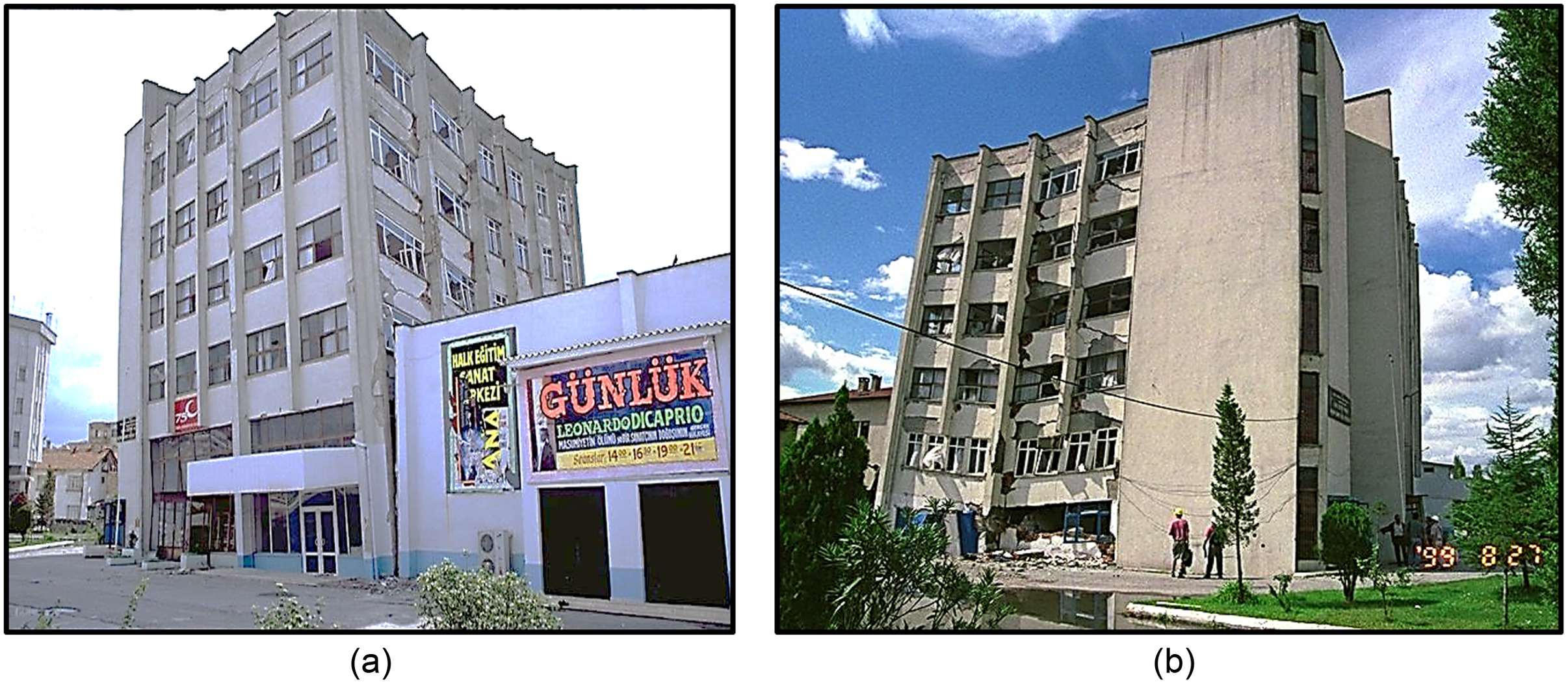
Fig. 4. Photos of PEC after EQ: (a) frontal view; and (b) rear view. (Images courtesy of NISEE-PEER Library, UC Berkeley.)

Image analysis of available reconnaissance photos using both the MATLAB (The Mathworks 2022) image processing toolbox and Autocad identified settlements of 0.25–0.3 m relative to the surrounding foot path, 0–0.04 rad of foundation tilt, and 0.07–0.14 rad of residual building drift. Note that the authors recognize the difficulty of discerning whether the rotation was due to building drift or foundation tilt. Notably, settlements of nearby buildings were between 0.20 and 0.90 m, but resulted in negligible structural damage since they were on raft foundations (Sancio 2003). The PEC building was demolished and a new building is now located at the same site.

Information about the Building

The PEC building was a 1970s five-story reinforced concrete building with about

200 m^{2}

in plan and isolated footings. The floor height was 4.9 m in the first floor and the upper floors were 3.4 m in height. The beams of the buildings were

0.45 m \times 0.70 m

. The interior columns were

0.45 m \times 0.45 m

, while the exterior columns were

0.45 m \times 0.70 m

. As seen in Fig. 4, there is a shear wall located in one of the corners of the building where the stairs were located. In the plan view, the arrangement of the footings and the columns is shown in Fig. 5(a). The footings were located at a depth of 1.3 m. All the footings were square in plan; the exterior footings were

1.75 m \times 1.75 m

and the interior footings were

1.5 m \times 1.5 m

. The tie beams were

0.30 m \times 0.30 m

.

Fig. 5. Plan view of the structural system (a) and the frame corresponding to section AA’ of the PEC building (b) including geometrical information (all dimensions are in meters).

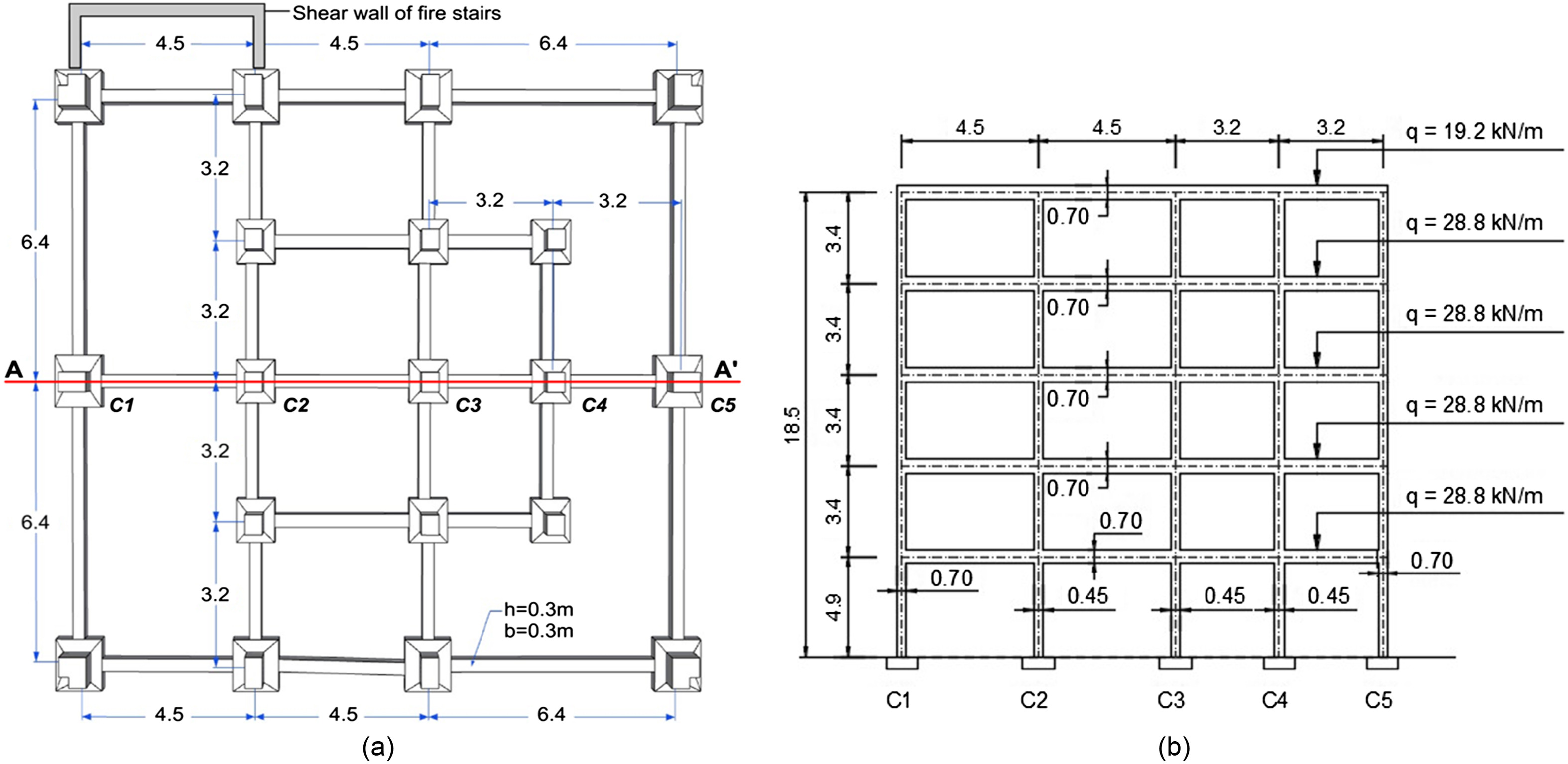
Since the two software packages used for the full model approach can only simulate two-dimensional models, the comparison study that was performed focuses only on the performance of the frame corresponding to section AA’ of the PEC building that is indicated in Fig. 5(a) and represented in Fig. 5(b). Since the as-built plans were not available for the building, and the purpose of the case study was only to compare the results obtained by different modelling approaches, the steel reinforcement of the elements of the AA’ frame was defined using a simulated design procedure compatible with 1970s design practice that considered gravity loads only. Fig. 5(b) presents the dimensions of the structural elements and the vertical loads corresponding to the quasi-permanent load combinations that are relevant for the performed seismic analyses. The quasi-permanent load combination was obtained from a permanent load of

6 kN / m^{2}

and a quasi-permanent value of the live load of

0.6 \times 5 kN / m^{2}

, according to the Turkish code from 1975 (TEC 1975). This distributed load was then transferred to the frame by considering a tributary width of 3.2 m, giving a distributed load for the seismic load case of

28.8 kN / m

for the stories and

19.2 kN / m

for the roof. The gravity load case used for estimating the reinforcing steel was taken as 1.5 times the sum of the permanent and live loads. The concrete design compressive strength and steel yield strength were 18 MPa and 230 MPa, respectively. The stiffness of the beams and columns was calculated using an assumed initial concrete stiffness of

E_{cm} = 26.2 MPa

and a cracked stiffness ratio of 0.5 was adopted for beams, where values between 0.35 and 0.46 were used for the columns depending on the axial load.

Soil Conditions and Ground Motion

Adapazari is located between the Sakarya and Cark Rivers and is settled mostly on Holocene alluvial deposits, which overlie older lake bed sediments. The groundwater level is very close to the ground surface at 1.0–3.0 m depth. The liquefiable layers are loose silty sands, sandy silts, and clayey silts (silt mixtures), which are generally in the first 10 meters (Sancio 2003; Bol et al. 2010). The normalized clean sand equivalent cone tip resistance (

q_{CINcs}

) values in these silty layers is small, in the range of 40–80, and generally less than 70.

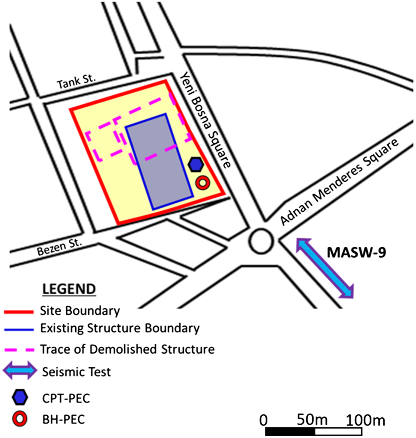
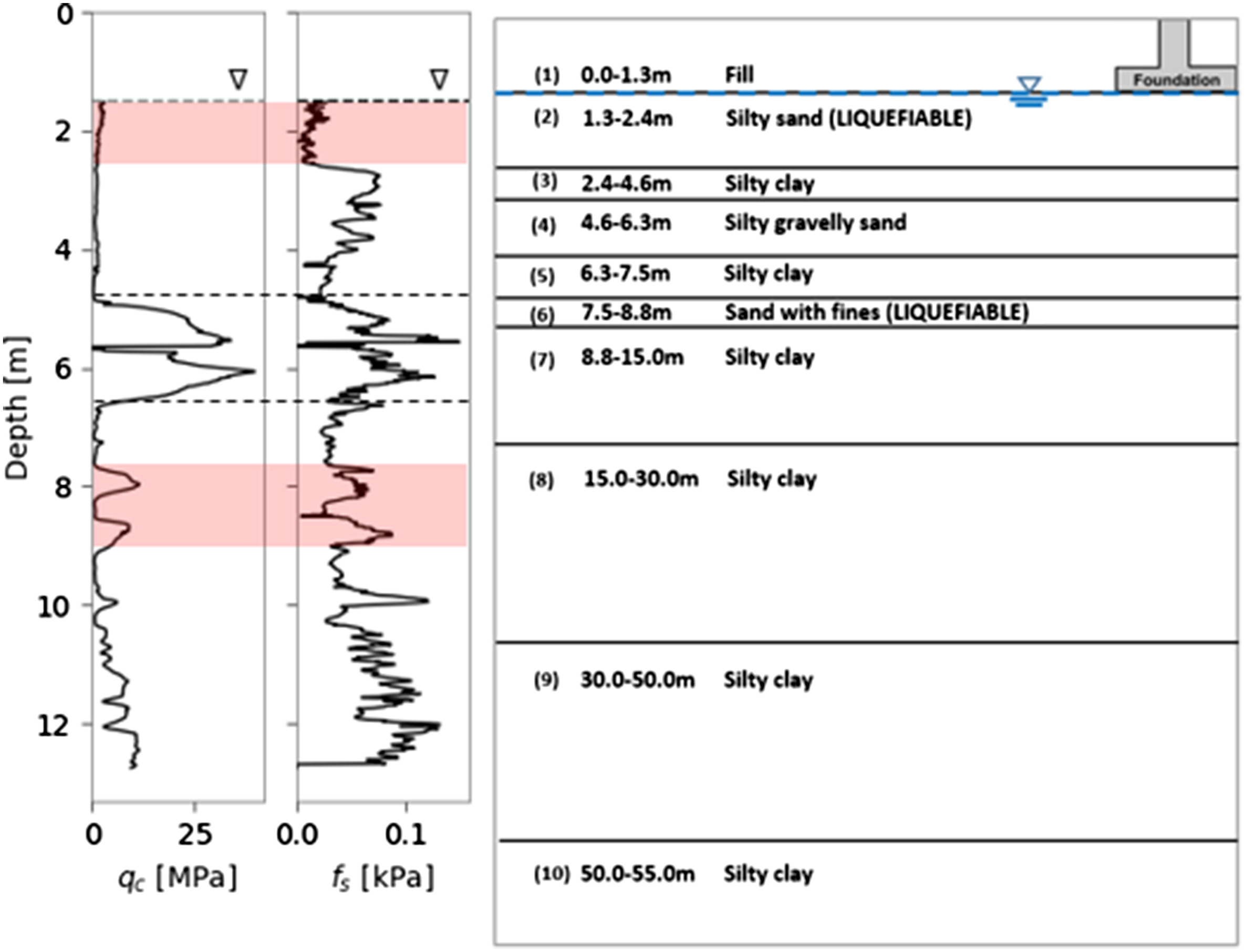
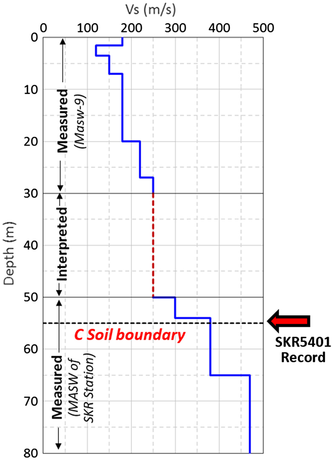
The soil profile below the PEC building was defined through CPTu, SPT, and seismic (MASW) tests (locations shown in Fig. 6). The CPTu test was carried out within the LIQUEFACT project (Lai et al. 2021) and the data of the SPT and laboratory tests and the velocity profile in the first 30 m (

V_{s, 30}

) were provided by the Sakarya Municipality. Fig. 7 shows the CPT data and idealized near surface soil profile at the PEC site. The subsoil consists of a total of 10 layers from which two are considered liquefiable, one non-plastic silt just below the foundation and another sand layer at 7.5 m. The groundwater level is at 1.3 m. The shear wave velocity profile from 30 m to the bedrock at 50 m was assumed to be the same as that at a 30-m depth. The soil at 50–80 m was assumed to be the same as that of the SKR recording station at around 3.6 km from the building.

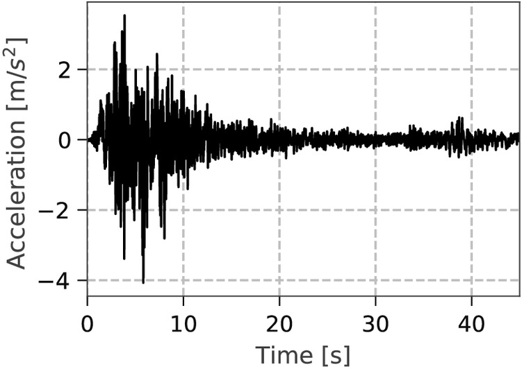
Fig. 6. Locations of site investigation tests.

Fig. 7. CPT data and idealized soil profile at the PEC site.

By interpreting the works of Komazawa et al. (2002) and Kudo et al. (2002), type C soil according to Eurocode 8 (CEN 2019) was accepted to lie at a depth of 55 m. Fig. 8 shows the

V_{s, 30}

profile at the PEC site based on the data provided by the Sakarya Municipality. Interpretation was then used to obtain the

V_{s}

profile between 30 m and 50 m. This is schematized in Fig. 8. The input motion considered for the analyses in the full numerical models and the ELSA method is the outcrop ground motion recorded at the SKR station in the EW direction, which had a PGA of 0.414 g, recorded on type C soil (Fig. 9).

Fig. 8. $V_{s}$ profile at PEC site and considered depths.

Fig. 9. Input motion (at 55 m depth) time series.

Full Model Approach

The “full model” approach that considers SLFSI was implemented in two different software packages (FLAC and PLAXIS) through a nonlinear dynamic soil-structure interaction effective stress analysis.

Description of the Full FLAC Numerical Model

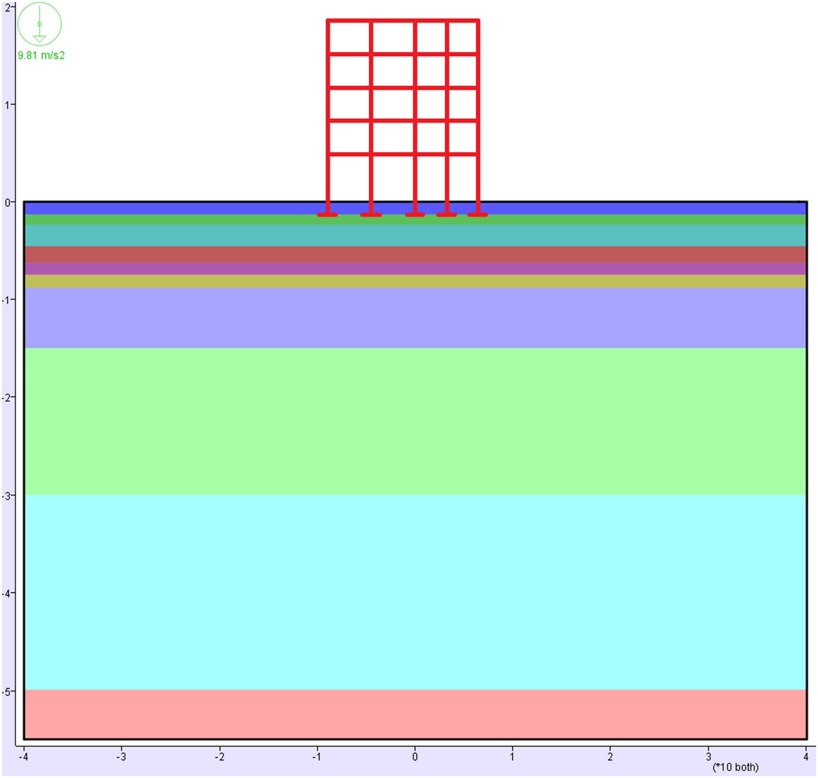
In FLAC, the soil mesh was consistent with the soil profile outlined in Fig. 10, with element sizes of approximately 0.4 m by 0.4 m near the building which were gradually coarsened to 0.7 m wide at the model edge. The total mesh was 55 m deep and 80 m wide (shown in Fig. 10), the lateral boundaries were tied together and the base boundary was a compliant base (absorbing) where the SSK-recorded motion was entered as a stress. Additional analyses were performed with a 200-m wide model in PLAXIS and some minor changes in pore pressure build up, surface acceleration, and differential settlement were observed; however, the smaller model was selected due to the long run time (

\sim 8 days

) of the model. The soil was modelled with only two constitutive models, the PM4Sand model (Boulanger and Ziotopoulou 2017) for liquefiable sands (second and sixth layers), and a Mohr–Coulomb model with hysteretic damping for the non-liquefiable soils. The default hysteretic damping model available in FLAC was used for the non-liquefiable layers to provide a more realistic stress-strain response. The extreme values of logarithmic strain (the values at which the tangent slope become zero), L1 and L2 parameters, were estimated as

1.7 \cdot {IP}^{0.5} - 3.6

and

- 1.2 \cdot {IP}^{0.5} + 2.25

, respectively, based on curve fitting to the modulus reduction curves from Vardanega and Bolton (2013), where IP is the plasticity index. The use of the simple Mohr–Coulomb model for the non-liquefiable layers was justified due to the amplitude of shear stresses applied to these layers in preliminary studies being less than what might result in significant strain softening and deformation. Non-liquefiable layers were modelled initially as undrained material but when the ground motion started, the ground water flow was activated allowing partial pore water pressure dissipation. Before applying the ground motion, a Mohr–Coulomb constitutive model was used in all 10 layers to calculate the initial stresses in the soil profile (Table 1 presents the Mohr–Coulomb parameters). The strength parameters of the top 20 meters were designated via CPT of the site and laboratory tests of Sancio (2003). For the deeper layers, strength parameters were estimated by using ’the previous reports of the Sakarya Municipality (2014) and by extrapolating the ratio 0.6 for the undrained strength over the vertical stress ratio from the deepest known value (at 30 m). Small strain stiffness parameters were derived from the

V_{s}

profile of the site. Secant and oedometer moduli were estimated using empirical relationships proposed by Alpan (1970) and PLAXIS (Bentley 2020). An additional 1.5% Rayleigh damping was specified at 1.14 Hz and 5 Hz to mitigate numerical instability.

Table 1. Input parameters of the Mohr–Coulomb model (FLAC)

Parameter	Unit	Layer
Parameter	Unit	1	2	3	4	5	6	7	8	9	10
H	m	1.3	1.1	2.2	1.7	1.2	1.3	6.2	15.0	20.0	5.0
$ρ$	$kg / m^{3}$	1,975	1,857	1,786	1,980	1,786	1,898	1,908	1,878	1,918	2,031
G	MPa	71	38	38	134	46	97	110	108	162	325
K	MPa	214	82	113	402	137	210	331	325	485	975
$ϕ^{'}$	degrees	0	33	0	36	0	33	0	0	0	—
c'	kPa	15	0	50	0	35	0	75	216	323	—
n	—	0.27	0.48	0.54	0.42	0.54	0.45	0.47	0.48	0.46	0.39
k	$m / s$	$2 \times 10^{- 3}$	$4 \times 10^{- 5}$	$9 \times 10^{- 8}$	$1 \times 10^{- 5}$	$6 \times 10^{- 8}$	$6 \times 10^{- 8}$	$2 \times 10^{- 8}$	$3 \times 10^{- 9}$	$1 \times 10^{- 9}$	$1 \times 10^{- 9}$

Note: H = height; ρ = density; G = shear modulus; B = bulk modulus; $φ$ = angle of shear resistance; c' = effective cohesion; n = porosity; and k = permeability.

The building elements were modelled as beam elements, which can only simulate elastic behavior (Fig. 10). The beam and footing elements were modelled with the provided dimensions and a Young’s modulus of 26.2 GPa. The secant-to-yield stiffness of the beams and columns was modelled according to the proposal of Haselton et al. (2016), which reduces the gross stiffness of a member to simulate the effect of cracking and accounts for the level of axial force. The secant-to-yield stiffness of the members was around 35%–50% of their gross stiffness, which is consistent with other proposals (Paulay and Priestley 1992; EPPO 2017). Since the FLAC software models the soil as a 2D mesh with a 1-m out-of-plane length, the foundation impedances and bearing capacities are less than what would be computed for a 3D footing using the correct footing width. While FLAC provides a spacing parameter to allow for scaling of loads and masses of structural elements, it is impossible to accurately match both the vertical and rotational stiffnesses, as well as the bearing capacity, with a single spacing value. Furthermore, the soil properties (particular frictional angle and shear modulus) are both dependent on whether the soil is loaded in plane strain on under 3D loading. Finally, it should be noted that the pore water flow could not escape in the out-of-plane direction. Given these limitations with converting a 3D model to a plane-frame superstructure on a plane strain soil, the 1-m out-of-plane length was used unscaled, compared to the 1.5-m out-of-plane width of the foundation, reducing the bearing capacity by 22% when applying the method from Salgado (2008). This simplification allowed the internal forces to be directly compared with PLAXIS results. The interface between the base of the footing elements and surrounding soil was fixed. However, the use of unglued interface elements was also tested in alternative analyses, but no significant slip or uplift was observed. The column elements below the ground level were not attached to the soil mesh.

Description of Full PLAXIS Numerical Model

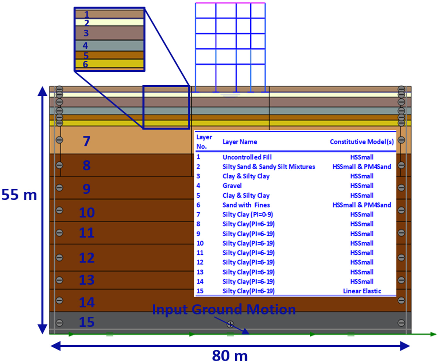
In PLAXIS, the soil mesh was consistent with the soil profile outlined in Fig. 11, where the finite element sizes were defined using the PLAXIS automated meshing algorithm using a minimum shear wave velocity of

120 m / s

and frequency of over 10 Hz. Additionally, mesh refinement was adopted below footings. The depth and width of the numerical model were taken as 55 m and 80 m, respectively, which was the same for the FLAC analyses. Prior to the dynamic loading phase, soil layers were modelled using the Hardening Soil with Small Strain (HSSmall) model for the definition of initial stress states and the subsequent structural loading phases. The soil model for the liquefiable second and sixth layers was switched to the PM4Sand model when the dynamic loading phase started. The parameters defining the HSSmall model for the soil layers are listed in Tables 2 and 3. Rayleigh damping was set at 1% at 1.2 Hz and 5 Hz based on the site period and strongest frequency of the input ground motion.

Table 2. Input parameters for layers 1 to 8 of the HSSmall and Linear Elastic models (PLAXIS)

Parameter	Unit	Layer
Parameter	Unit	1	2	3	4	5	6	7	8
Thickness	m	1.3	1.1	2.2	1.7	1.2	1.3	6.2	5
Unit weight	$kN / m^{3}$	19.4	17.8	17.5	19.4	18.5	18.7	18.8	18.4
$e_{0}$	—	1.1	0.96	0.96	0.36	0.52	0.92	0.83	0.45
E	MPa	—	—	—	—	—	—	—	—
$E_{oed}^{ref}$	MPa	11	6	6	34	7	19	24	23
$E_{50}^{ref}$	MPa	11	6	6	34	7	19	24	23
$E_{ur}^{ref}$	MPa	34	18	18	102	22	56	71	70
Cohesion, $c_{r e f}^{'}$	kPa	15	—	50	5	35	—	75	216
Friction angle, $ϕ^{'}$	degrees	—	33	—	36	—	33	—	—
$G_{0}^{ref}$	MPa	70	37	37	131	45	95	108	107
$γ_{0.7}$	—	$1 \times 10^{- 5}$	$1 \times 10^{- 4}$	$6 \times 10^{- 4}$	$9 \times 10^{- 5}$	$4 \times 10^{- 4}$	$2 \times 10^{- 4}$	$3 \times 10^{- 4}$	$5 \times 10^{- 4}$
Permeability	$m / s$	$2 \times 10^{- 3}$	$4 \times 10^{- 5}$	$9 \times 10^{- 8}$	$1 \times 10^{- 5}$	$6 \times 10^{- 8}$	$6 \times 10^{- 8}$	$4 \times 10^{- 8}$	$3 \times 10^{- 9}$

Table 3. Input parameters for layers 9 to 15 of the HSSmall and Linear Elastic models (PLAXIS)

Parameter	Unit	Layer
Parameter	Unit	9	10	11	12	13	14	15
Thickness	m	5	5	5	5	5	5	5
Unit weight	$kN / m^{3}$	18.4	18.4	18.6	18.8	18.8	18.9	21
$e_{0}$	—	0.44	0.45	0.42	0.42	0.41	0.4	0.5
E	MPa	—	—	—	—	—	—	1,073
$E_{oed}^{ref}$	MPa	23	23	42	41	54	54	—
$E_{50}^{ref}$	MPa	23	23	42	41	54	54	—
$E_{ur}^{ref}$	MPa	69	68	125	124	163	162	—
Cohesion, $c_{r e f}^{'}$	kPa	216	216	323	323	323	323	—
Friction angle, $ϕ^{'}$	degrees	—	—	—	—	—	—	—
$G_{0}^{ref}$	MPa	107	105	147	147	170	170	400
$γ_{0.7}$	—	$5 \times 10^{- 4}$	$5 \times 10^{- 4}$	$3 \times 10^{- 4}$	$3 \times 10^{- 4}$	$3 \times 10^{- 4}$	$3 \times 10^{- 4}$	—
Permeability	$m / s$	$3 \times 10^{- 9}$	$3 \times 10^{- 9}$	$1 \times 10^{- 9}$	$1 \times 10^{- 9}$	$1 \times 10^{- 9}$	$1 \times 10^{- 9}$	—

In the dynamic analysis, the lateral boundaries were tied together and the base boundary was a compliant base (absorbing) where the SKR-recorded motion was entered as a displacement. In order to provide a reasonable comparison of the two software packages, identical structural parameters were chosen in PLAXIS as well. The type of calculation used in PLAXIS was a dynamic analysis with consolidation. Initially, one-dimensional soil column models of the site in both FLAC and PLAXIS were developed to compare and validate the model inputs and water flow. The interface between the base of the footing elements and surrounding soil was fixed.

Soil Constitutive Modelling of Liquefiable Layer

The PM4Sand (version 3.1) constitutive model (Boulanger and Ziotopoulou 2017) was used in both the FLAC and PLAXIS models to simulate the liquefiable soil. The PM4Sand model follows the framework of the stress-ratio-controlled, critical state-compatible, bounding surface plasticity model for sand presented by Dafalias and Manzari (2004). The PM4Sand model has been used to successfully model case histories (Bray and Macedo 2017) and centrifuge tests (Boulanger et al. 2017; Ziotopoulou and Montgomery 2017), and recently, the authors simulated the centrifuge tests by Dashti et al. (2010) as part of the model validation (Viana da Fonseca et al. 2018).

The PM4Sand parameters for the upper liquefiable layer were based on the measured properties from Sancio (2003) and calibrated to best fit the hysteretic response of the cyclic simple shear tests, J5-P4B and D5-P1B-3, carried out by Sancio (2003) on similar Adapazari silts at similar stress levels [Figs. 12(a and b)]. The lower liquefiable layer was calibrated based on the median normalized clean sand tip resistance in the liquefiable layer of 105 from the CPT. For the CPT calibration, the equivalent liquefaction resistance curve adapted from Boulanger and Idriss (2016) and Appendix A of Boulanger and Idriss (2014) was used for calibration to 5% single amplitude shear strain and can be seen in Fig. 12(c). The upper liquefiable layer was therefore assigned the following PM4Sand properties: relative density

D_{r} = 43 %

, normalized shear modulus

G_{o} = 757

, contraction rate parameter

h_{p o} = 0.325

, maximum void ratio

e_{\max} = 1.2

, and minimum void ratio

e_{\min} = 0.55

. The lower liquefiable layer was assigned the following PM4Sand properties: relative density

D_{r} = 57 %

, normalized shear modulus

G_{o} = 757

, contraction rate parameter

h_{p o} = 0.086

, maximum void ratio

e_{\max} = 1.2

, and minimum void ratio

e_{\min} = 0.55

. All other PM4Sand properties were kept at their default values for both layers.

Fig. 12. Calibration of Layer 2 PM4Sand parameters through a comparison of real and simulated CDSS test results in terms of shear stress–shear strain for a test with a CSR of: (a) 0.41; (b) 0.33; and (c) calibration of Layer 6 PM4Sand parameters through a comparison with the B&I curve.

Implementation of the Macro-Mechanism Model

The key inputs for the structural model were developed according to the macro-mechanism approach outlined before, where the same input ground motion, soil profile, and building properties were used as in the full models. The

{NCASE}_{liq}

values of 0.005 and 0.002 were calculated from Eq. (11) (Viana da Fonseca et al. 2018), using a cyclic resistance ratio, CRR of 0.211 and 0.144 for number of cycles to liquefaction, n_liq of 15 and G of 38 MPa and 97 MPa for the two liquefiable layers, where

σ_{v 0}^{'}

is the vertical effective stress,

ϕ

is the angle of shearing resistance taken as 33°,

k = 3

and

s_{r, r u = 0} = 40

. The CRR for the upper liquefiable layer was obtained from interpolating a series of PM4Ssand element tests

{NCASE}_{l i q} = \frac{2 \cdot C R R^{2} \cdot σ_{v 0}^{'} \cdot n_{l i q}}{G \cdot (1 - \frac{C R R \cdot s_{r, r u = 0}}{\tan (ϕ) \cdot (1 + s_{r, r u = 0})})} \cdot κ

(11)

Note that in the macro-mechanism approach, the foundation impedances could be modelled based on the actual three-dimensional size, therefore the spring stiffnesses of the vertical, horizontal, and rotational degrees of freedom were

349 kN / m

,

444 kN / m

, and

167 kN / m

, respectively, compared to their 2D equivalents in the full models of

87 kN / m

,

87 kN / m

, and

97 kN / m

, respectively.

The structural model was implemented in the open-source software OpenSees (McKenna et al. 2010) using a lumped plasticity modelling technique to capture the nonlinear deformation of the beams, columns, joints, infills, and soil-foundation interface (as shown in Fig. 13). This software framework uses the finite element method to simulate the response of structural and geotechnical systems subjected to earthquakes.

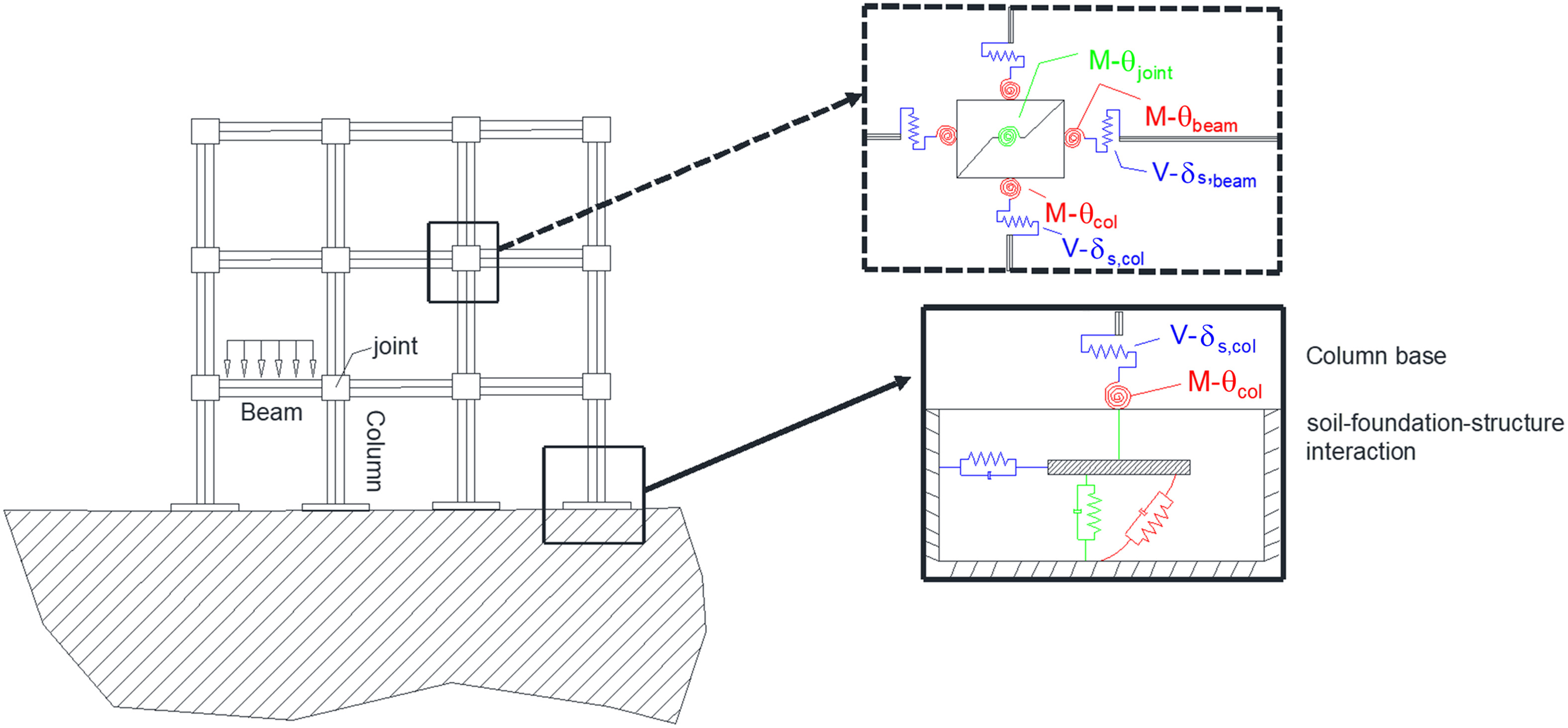
Fig. 13. Representation of the considered structural modelling approach.

The numerical model of the RC frame was assembled using frame elements and a scissor’s model was used for the beam-column joints, with the latter following the proposal and numerical implementation details presented in Altoontash (2004). The flexural inelastic behavior of the beams and columns of the RC frame was simulated using a set of rotational springs located on both ends of all structural elements connected in series with an elastic frame element. The hysteretic flexural behavior of these springs was defined by a moment-rotation law following a backbone curve constructed using the yielding moment (My) computed according to Panagiotakos and Fardis (2001), and the initial stiffness, capping moment (Mcap) and also the capping (θcap) and the ultimate (θu) rotation ductility values computed according to Haselton et al. (2016). The properties of the backbone curve of all columns were determined considering the axial force due to vertical loads of the quasi-permanent load combination. The effective stiffness of the frame elements was taken as the cracked stiffness. Stiffness and strength and unloading stiffness degradation are considered in the hysteresis curves. To account for the possibility of shear failure in the RC frame elements, a shear spring was added in series to these elements, considering the shear failure detection model proposed in Elwood and Moehle (2003) and Elwood (2004) and performed in post-processing. Particularly, a limit state model (Elwood and Moehle 2003) considering a generic three-point limit curve was adopted using the shear capacity according to the model provided in the Eurocode 8-Part 3 (CEN 2005). Moreover, a model proposed by Baradaran Shoraka et al. (2013) was used to simulate the non-ductile shear strength degradation. The hysteretic response of the beam-column joints was modelled following the proposal by O’Reilly and Sullivan (2019). P-delta effects were simulated using a leaning column. A damping factor of 3% of critical damping in the first and third modes of the structure was adopted using the tangent stiffness proportional Rayleigh damping model.

At the base of the frame, an additional set of nonlinear springs and dashpots was defined to incorporate SLFSI. The expected level of settlement in each footing was imposed at the base of the vertical spring. The surface ground motion was determined using the ELSA method, representing the near-field soil motion, and was imposed at the end of the horizontal spring not attached to the foundation.

Comparison of Modelling Approaches

To both validate the numerical models and evaluate the performance of the macro-mechanism approach, several different simulations were run. Both full effective stress 2D numerical models in FLAC and PLAXIS software were run with the nonlinear soil models and a linear elastic model of the building to provide an indication of the variation and sensitivity of the results of these models. The same modelling assumptions were implemented in both models when possible. The OpenSees model was then run with nonlinear structural members using the simplified methods described in the macro-mechanism section above as inputs for the macro-mechanism calculations (scenario named OS-NL-w-SMI). Finally, an intermediate model was considered, where the OpenSees model was analyzed with an elastic superstructure using footing springs and dashpots based on equivalent 2D strip footing, and using the outputs from FLAC (surface ground motion, footing settlements and pore pressure in the middle of the liquefiable layer) as the input values for the macro-mechanism calculations (scenario named OS-Lin-w-FI). This model has been considered as a reference to evaluate the decoupling of the models, as a direct comparison can be made with the FLAC model, where the structure is also modelled with elastic elements.

It should be noted that while the macro-mechanism approach is intended for use with simple models to define the inputs, the approach is modular and, therefore, inputs can be defined using advanced effective stress analysis. In this case the main advantage is the decoupling of the structural analysis from the soil analysis to allow for greater detail in the structural analysis that cannot be achieved with most commercial software capable of effective stress analysis.

Fig. 14(a) shows the surface acceleration time series and b) the surface response spectrum from each method. From Fig. 14, it can be seen that the PLAXIS surface acceleration response was higher than the FLAC response, particularly at 7–8 s, which resulted in a higher spectral response across all response periods. The ELSA method provides demand levels very similar to FLAC across both time and frequency.

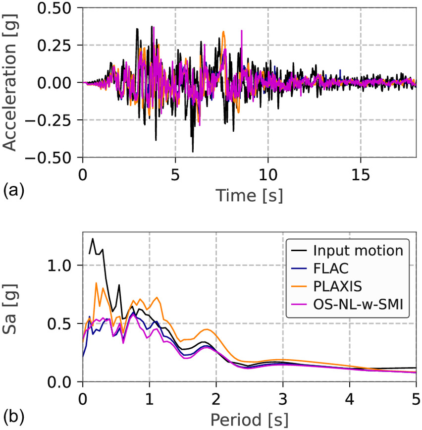
Fig. 14. (a) Surface acceleration time series; and (b) corresponding spectral acceleration.

Fig. 15 presents several key time series. In Fig. 15(a), the first-floor inter-story drift time series shows that the FLAC, PLAXIS and OS-Lin-w-FI peak deformations were fairly similar; however, the residual behavior was different. The difference in residual deformation here is due to differences in the relative movement of the exterior footings with respect to the central footing caused by local soil deformation, as the structural elements are modelled as elastic in these three models. Note that the inter-story drift was computed as the relative horizontal displacement in the first floor in relation to the central footing, minus the global foundation tilt (differential settlement of the exterior footings divided by the distance between them). A further difference between the OS-Lin-w-FI model and the FLAC model is caused by the difference in foundation impedances where the OS-Lin-w-FI model adopts the impedances from Karatzia et al. (2017). A notable difference in behavior is seen in the OS-NL-w-SMI model, where both peak and permanent deformations are considerably larger. Even though the shaking demand was seen to be similar between the ELSA method and the two full effective stress models, the yielding of the nonlinear structural elements has resulted in remarkably different behavior. While the residual drift value was less than the observed range (0.07–0.14 rad), the shear and axial failures that were observed in the real building were not directly modelled in this analysis and were only assessed in post-processing.

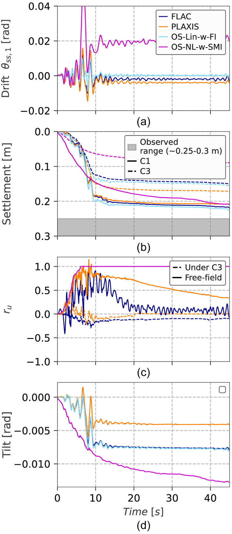
Fig. 15. Comparison between the different numerical models: (a) first-floor inter-story drift; (b) settlements at C1 and C3 column; (c) excess pore pressure ratio in the middle of the liquefiable layer in free-field and under each column; and (d) tilt.

In Fig. 15(b), the shear-induced settlements below columns 1 and 3 (see Fig. 15 for numbering) are shown. While the settlements in all four models are similar, the PLAXIS model exhibits less differential movement than the FLAC model, and the OS-NL-w-SMI model has larger differential movement, which is due to the applied tilt. The rate of settlement of the OS-NL-w-SMI is also inconsistent with the other models, because the settlement rate in this model is only dependent on CAVdp. Considering that a time-dependent LBS in Eq. (4) does reduce the initial rate of settlement, which is reflected in the soil not being liquefied, the deformation will be less. Overall, the shear-induced settlement of all four models was similar but less than the observed range of 0.25–0.3 m. Additional volumetric based settlement using the method from Zhang et al. (2004) was computed as 0.06 m. Following the procedure from Bray and Macedo (2017), there was a low likelihood of sediment ejecta (largely consistent with field photos) when evaluating the soil profile against the ground failure chart from Ishihara (1985), therefore ejecta-based settlement was assumed negligible. Considering the contributions from both shear-induced and volumetric settlement, the total settlement from all models was comparable to observations.

In Fig. 15(c), the pore pressure ratio in the middle of the uppermost liquefiable layer for free-field conditions and under the central footing is shown. In all models the pore pressure build up was reasonably similar and reached a state of liquefaction in the free-field, consistent with the observed soil ejecta near the building. Finally, the global foundation tilt is shown in Fig. 15(d), where it can be seen that the PLAXIS model had less tilt than the FLAC model, while the OS-NL-w-SMI model had significantly more. Note that the OS-NL-w-SMI model uses the empirical tilt expression from Bullock et al. (2019a), which is based on field observations. Bullock et al. (2019a) notes that the empirical model tends to predict larger tilt than estimated from numerical simulations, since numerical simulations do not fully capture the effects of 3D heterogeneity and soil ejecta, thus consistent with the findings here. All models resulted in foundation tilt values within the observed range, noting the difficulty in obtaining exact tilt values from image analysis.

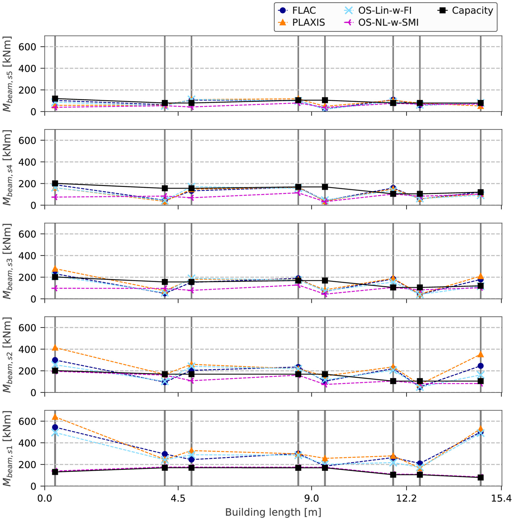
The four models (FLAC, PLAXIS, OpenSees-Linear-w-FI, and OpenSees-Nonlinear-w-SMI) were also compared in terms of maximum moment demands in the beams (Fig. 16) and columns (Fig. 17). As expected, the FLAC, PLAXIS, and OS-Lin-w-FI model produce similar demands, where the discrepancies are mainly associated with minor differences in foundation impedances between the mesh and springs, as well as mass distribution and damping. The demands from the OS-NL-w-SMI model are notably different, especially in the lower stories. The beam demands closely follow the section capacity values indicating that they have yielded. Since the elastic structural models do not account for the yielding of structural elements, the nonlinear model provides a more reasonable estimate of overall deformation and damage. Finally, each beam and column end was evaluated against shear failure in post-processing for the nonlinear model. No shear failures were observed in the beams (note none were reported from field observations either); however, several shear failures were observed in the lower stories and are consistent with the field findings.

Fig. 16. Comparison of maximum beams moment demand from: PLAXIS and FLAC full model approaches, the linear structural model in OpenSees using FLAC outputs (OS-Lin-w-FI), and nonlinear structural model in OpenSees using the outputs from the simplified approaches selected for the macro-mechanism (OS-NL-w-SMI).

Fig. 17. Comparison of maximum columns moment demand from: PLAXIS and FLAC full model approaches, the linear structural model in OpenSees using FLAC outputs (OS-Lin-w-FI), and nonlinear structural model in OpenSees using the outputs from the simplified approaches selected for the macro-mechanism (OS-NL-w-SMI).

While no model exactly replicated the observed outcome of the building in terms of settlement, tilt, drift, and structural damage, the uncertainty in the ground motion, building properties, soil properties (and soil heterogeneity) as well as the simplification adopted in only modelling a single frame of the building in 2D are certainly sources of the discrepancies. The ability of the macro-mechanism approach to provide more detailed nonlinear modelling of structural elements and 3D foundation impedances resulted in the model providing additional insight into the building performance compared to the two full model approaches. Furthermore, it is noted that the full model numerical analyses are very time consuming in terms of computation time (the FLAC full model took about 8 days and the PLAXIS full model about 6 hours, both run on the same desktop computer with 3.3 GHz and 10 cores, while the macro-mechanism approach takes less than 5 minutes to execute (both developing the estimation of the macro-mechanism inputs and running the nonlinear time history analysis) once the models are scripted to pass outputs as inputs into subsequent models. The reduced run time allows some of the known sources of uncertainty to be addressed parametrically.

The fast run time, consideration of nonlinear behavior, and the ability to account for epistemic uncertainty through different models makes the macro-mechanism approach an ideal method for carrying out probabilistic seismic performance analysis and developing fragility curves of buildings considering the effects of liquefaction. However, further research would improve the application of the method, particularly in understanding how total and differential settlement, as well as tilt, manifest in irregular buildings with isolated footings and in heterogeneous soil conditions.

Conclusions

The numerical simulation of full buildings on liquefiable soil during strong shaking is a highly demanding task for any engineer. This article presents four different simulations of a case study of a building during the Adapazari 1999 earthquake to outline the key steps involved and comparative differences in the output. The first two approaches consist of full effective stress 2D numerical models of the soil domain with equivalent linear structural models to represent the building. The first model was developed in the finite difference software FLAC and the second model in the finite element software PLAXIS. Where possible, the two models used the same modelling assumptions (i.e., same geometry, structural properties, liquefiable soil constitutive model). However, due to inherent differences in the software, there were differences in the mesh, solving algorithms, and constitutive models for the non-liquefiable clay layers. The two models were developed with the intention of providing an indication of the variation and sensitivity of the results of 2D effective stress models. The other two models were developed in OpenSees and simulated the liquefiable soil deposit using the outlined macro-mechanism approach. In the macro-mechanism approach, the influence of the liquefiable soil on the building is quantified in terms of its changes to the ground surface acceleration, the soil-foundation impedance and the settlement of the footings. Several analytical and empirical models were applied to estimate these quantities such that they could be simulated as a series of springs, dashpots, and imposed displacements. The first of the macro-mechanism models used identical structural properties as the FLAC and PLAXIS models to allow for direct comparison, whereas the final model took full advantage of the advanced constitutive models for structural elements and attempted to directly model the nonlinear aspects of the superstructure.

The results of this study highlight that:

1.

There is reasonable agreement between the two full model approaches even though two completely different software programs were used.

2.

The simplified model to estimate free-field pore pressure produced estimated values very similar to those of the effective stress models.

3.

The simplified model for the surface ground motion for use in the macro-mechanism approach produced very similar demands to the FLAC analysis, whereas the PLAXIS analysis produced higher demands.

4.

The simplified model for settlement produced a reasonably similar estimate to the two effective stress analyses, i.e., 60% of the FLAC model, and 50% of the PLAXIS model with respect to the central footing.

5.

The simplified tilt model produced larger values than the simulations, as expected due to it being calibrated to field data, reflecting that numerical simulations tend to under predict observed tilt.

6.

The use of nonlinear structural elements resulted in markedly different deformation, element demands, and damage compared to the linear elements used in the other models.

7.

Overall, the macro-mechanism model provided a reasonable estimate of the observed damage to the building in terms of column failures and permanent deformation at the foundation level addressing some of the shortfalls of using analyses with an elastic plane-frame on a plane-strain soil domain.

Data Availability Statement

•

Some or all data, models, or code generated or used during the study are available in a repository or online in accordance with funder data retention policies. The code for calculating the cyclic resistance ratio and equivalent liquefaction resistance curve according to Boulanger and Idriss (2014) can be found in the Liquepy package version 0.6.24 at: https://github.com/eng-tools/Liquepy/blob/master/Liquepy/trigger/boulanger_and_idriss_2014.py.

The code for performance liquefaction triggering according to the strain energy method from Millen et al. (2020) can be found at: https://github.com/eng-tools/Liquepy/blob/master/Liquepy/trigger/nses.py. The code for performing the Equivalent Linear Stockwell Analysis can be found at: https://github.com/eng-tools/Liquepy/blob/master/Liquepy/sra/elsa.py. The code for calculating shear-induced foundation settlement according to Bray and Macedo (2017) can be found at: https://github.com/eng-tools/Liquepy/blob/master/Liquepy/settlement/methods.py. The code for calculating volumetric based settlement according to (Zhang et al. 2004) can be found here: https://github.com/eng-tools/Liquepy/blob/master/Liquepy/trigger/volumetric_strain.py. Damage patterns and photos of the PEC building can be found at https://nisee.berkeley.edu/elibrary/

•

Some or all data, models, or code used during the study were provided by a third party. Data on the building and the MASW test was provided by Sakarya Municipality and additional information was provided by Adapazari Municipality. Direct request for these materials may be made to the provider as indicated in the Acknowledgments.

Acknowledgments

This paper was produced as part of the LIQUEFACT project (“Assessment and mitigation of liquefaction potential across Europe: a holistic approach to protect structures/infrastructures for improved resilience to earthquake-induced liquefaction disasters”), which has received funding from the European Union’s Horizon 2020 research and innovation programme under Grant Agreement No. GAP-700748. This work was financially supported by: Base Funding—UIDB/04708/2020 and Programmatic Funding—UIDP/04708/2020 of the CONSTRUCT—Instituto de I&D em Estruturas e Construções—funded by national funds through the FCT/MCTES (PIDDAC). The third author acknowledges the support of FCT through the Grant SFRH/BD/143817/2019. The fifth author also acknowledges the support of FCT through the grant CEECIND/04583/2017. The authors would also like to acknowledge the Adapazari and Sakarya Municipalities for providing access and information related to the site.

References

Alpan, I. 1970. “The geotechnical properties of soils.” Earth Sci. Rev. 6 (1): 5–49. https://doi.org/10.1016/0012-8252(70)90001-2.

Google Scholar

Altoontash, A. 2004. “Simulation and damage models for performance assessment of reinforced concrete beam-column joints.” Ph.D. dissertation, Dept. of Civil and Environmental Engineering, Stanford Univ.

Google Scholar

Baradaran Shoraka, M., T. Y. Yang, and K. J. Elwood. 2013. “Seismic loss estimation of non-ductile reinforced concrete buildings.” Earthquake Eng. Struct. Dyn. 42 (2): 297–310. https://doi.org/10.1002/eqe.2213.

Google Scholar

Bay, J. A., and B. R. Cox. 2001. Shear wave velocity profiling and liquefaction assessment of sites shaken by the 1999 Kocaeli, Turkey Earthquake. Logan, UT: Utah State Univ.

Google Scholar

Bentley. 2020. “Plaxis2D, Complete 2D geotechnical analysis software version: 21.” Accessed March 1, 2022. https://www.bentley.com/en/products/product-line/geotechnical-engineering-software/plaxis-2d.

Google Scholar

Bird, J. F., J. J. Bommer, H. Crowley, and R. Pinho. 2006. “Modelling liquefaction-induced building damage in earthquake loss estimation.” Soil Dyn. Earthquake Eng. 26 (1): 15–30. https://doi.org/10.1016/j.soildyn.2005.10.002.

Google Scholar

Bol, E., A. Onalp, E. Arel, S. Sert, and A. Ozocak. 2010. “Liquefaction of silts: The Adapazari criteria.” Bull. Earthquake Eng. 8 (4): 859–873. https://doi.org/10.1007/s10518-010-9174-x.

Google Scholar

Boulanger, R., C. Curras, B. Kutter, D. Wilson, and A. Abghari. 1999. “Seismic soil-pile-structure interaction experiments and analyses.” J. Geotech. Geoenviron. Eng. 125 (9): 750–759. https://doi.org/10.1061/(ASCE)1090-0241(1999)125:9(750).

Google Scholar

Boulanger, R., and K. Ziotopoulou. 2017. PM4Sand (Version 3.1): A sand plasticity model for earthquake engineering applications. Berkeley, CA: Univ. of California at Davis.

Google Scholar

Boulanger, R. W., and I. M. Idriss. 2014. “CPT and SPT based liquefaction triggering procedures. Technical Rep. No. UCD/CGM-14, 1. Berkeley, CA: Univ. of California at Davis.

Google Scholar

Boulanger, R. W., and I. M. Idriss. 2016. “CPT-based liquefaction triggering procedure.” J. Geotech. Geoenviron. Eng. 142 (2): 04015065. https://doi.org/10.1061/(ASCE)GT.1943-5606.0001388.

Google Scholar

Boulanger, R. W., M. Khosravi, A. Khosravi, D. W. Wilson, A. Pulido, and W. Yunlong. 2017. “Remediation of liquefaction effects for a dam using soil-cement grids: Centrifuge and numerical modeling.” In Proc., 19th Int. Conf. on Soil Mechanics and Geotechnical Engineering, 2477–2480. London: International Society for Soil Mechanics and Geotechnical Engineering.

Google Scholar

Bray, J., and J. Macedo. 2017. “6th Ishihara lecture: Simplified procedure for estimating liquefaction induced building settlement.” Soil Dyn. Earthquake Eng. 102 (Nov): 215–231. https://doi.org/10.1016/j.soildyn.2017.08.026.

Google Scholar

Bullock, Z., S. Dashti, Z. Karimi, A. Liel, K. Porter, and K. Franke. 2019a. “Probabilistic models for residual and peak transient tilt of mat-founded structures on liquefiable soils.” J. Geotech. Geoenviron. Eng. 145 (2): 04018108. https://doi.org/10.1061/(ASCE)GT.1943-5606.0002002.

Google Scholar

Bullock, Z., Z. Karimi, S. Dashti, K. Porter, A. B. Liel, and K. W. Franke. 2019b. “A physics-informed semi-empirical probabilistic model for the settlement of shallow-founded structures on liquefiable ground.” Géotechnique 69 (5): 406–419. https://doi.org/10.1680/jgeot.17.P.174.

Google Scholar

Campbell, K. W., and Y. Bozorgnia. 2012. “A comparison of ground motion prediction equations for arias intensity and cumulative absolute velocity developed using a consistent database and functional form.” Earthquake Spectra 28 (3): 931–941. https://doi.org/10.1193/1.4000067.

Google Scholar

CEN (European Committee for Standardization). 2005. Design of structures for earthquake resistance. Part 3: Assessment and retrofitting of buildings. Eurocode 8. Brussels, Belgium: CEN.

Google Scholar

CEN (European Committee for Standardization). 2019. Eurocode 8: Design of structures for earthquake resistance, Part 1. Brussels, Belgium: CEN.

Google Scholar

Dafalias, Y., and M. Manzari. 2004. “Simple plasticity sand model accounting for fabric change effects.” J. Eng. Mech. 130 (6): 622–634. https://doi.org/10.1061/(ASCE)0733-9399(2004)130:6(622).

Google Scholar

Darendeli, B. M. 2001. “Development of a new family of normalized modulus reduction and material damping curves.” Ph.D. dissertation, Dept. of Civil, Architectural, and Environmental Engineering, Univ. of Texas at Austin.

Google Scholar

Dashti, S., and J. D. Bray. 2013. “Numerical simulation of building response on liquefiable sand.” J. Geotech. Geoenviron. Eng. 139 (8): 1235–1249. https://doi.org/10.1061/(ASCE)GT.1943-5606.0000853.

Google Scholar

Dashti, S., J. D. Bray, J. M. Pestana, M. Riemer, and D. Wilson. 2010. “Centrifuge testing to evaluate and mitigate liquefaction-induced building settlement mechanisms.” J. Geotech. Geoenviron. Eng. 136 (7): 918–929. https://doi.org/10.1061/(ASCE)GT.1943-5606.0000306.

Google Scholar

Elwood, K. J. 2004. “Modelling failures in existing reinforced concrete columns.” Can. J. Civ. Eng. 31 (5): 846–859. https://doi.org/10.1139/l04-040.

Google Scholar

Elwood, K. J., and J. P. Moehle. 2003. Shake table tests and analytical studies on the gravity load collapse of reinforced concrete frames. Berkeley, CA: Univ. of California.

Google Scholar

EPPO (Earthquake Planning and Protection Organization of Greece). 2017. Greek code for interventions (KANEPE). [In Greek.] Athens, Greece: EPPO.

Google Scholar

FEMA. 2003. “Multi-hazard loss estimation methodology.” In HAZUS-MH technical manual. Washington, DC: FEMA.

Google Scholar

Fotopoulou, S., S. Karafagka, and K. Pitilakis. 2018. “Vulnerability assessment of low-code reinforced concrete frame buildings subjected to liquefaction-induced differential displacements.” Soil Dyn. Earthquake Eng. 110 (Jun): 173–184. https://doi.org/10.1016/j.soildyn.2018.04.010.

Google Scholar

Gazetas, G. 1991. “Foundation vibrations.” In Foundation engineering handbook, 553–593. New York: Springer. https://doi.org/10.1007/978-1-4757-5271-7_15.

Crossref

Google Scholar

Gómez-Martinez, F., M. D. L. Millen, P. A. Costa, and X. Romão. 2020. “Estimation of the potential relevance of differential settlements in earthquake-induced liquefaction damage assessment.” Eng. Struct. 211 (Jun): 110232. https://doi.org/10.1016/j.engstruct.2020.110232.

Google Scholar

Green, R. A., J. K. Mitchell, and C. Polito. 2000. “An energy-based excess pore pressure generation model for cohesionless soils.” In Proc., John Booker Memorial Symp., edited by P. Balkema. Rotterdam, Netherlands: A.A. Balkema.

Google Scholar

Haselton, C. B., A. B. Liel, S. C. Taylor-Lange, and G. G. Deierlein. 2016. “Calibration of model to simulate response of reinforced concrete beam-columns to collapse.” ACI Struct. J. 113 (6): 1141–1152. https://doi.org/10.14359/51689245.

Google Scholar

Ishihara, K. 1985. “Stability of natural deposits during earthquakes.” In Vol. 1 of Proc., 11th Int. Conf. on Soil Mechanics and Foundation Engineering, 321–376. Rotterdam, Netherlands: A.A. Balkema.

Google Scholar

Itasca. 2016. FLAC, fast Lagrangian analysis of continua v8.0.438. Minneapolis: Itasca Consulting Group.

Google Scholar

Karamitros, D. K., G. D. Bouckovalas, and Y. K. Chaloulos. 2013. “Seismic settlements of shallow foundations on liquefiable soil with a clay crust.” Soil Dyn. Earthquake Eng. 46 (3): 64–76. https://doi.org/10.1016/j.soildyn.2012.11.012.

Google Scholar

Karatzia, X., G. Mylonakis, and G. Bouckovalas. 2017. “Equivalent-linear dynamic stiffness of surface footings on liquefiable soil.” In Proc., 6th Int. Conf. on Computational Methods in Structural Dynamics and Earthquake Engineering, 1388–1402. Athens, Greece: National Technical Univ. of Athens.

Google Scholar

Karatzia, X., G. Mylonakis, and G. Bouckovalas. 2019. “Seismic isolation of surface foundations exploiting the properties of natural liquefiable soil.” Soil Dyn. Earthquake Eng. 121 (Jun): 233–251. https://doi.org/10.1016/j.soildyn.2019.03.009.

Google Scholar

Kokusho, T. 2013. “Liquefaction potential evaluations: Energy-based method versus stress-based method.” Can. Geotech. J. 50 (10): 1088–1099. https://doi.org/10.1139/cgj-2012-0456.

Google Scholar

Komazawa, M., H. Morikawa, K. Nakamura, J. Akamatsu, K. Nishimura, S. Sawada, A. Arken, and A. Onalp. 2002. “Bedrock structure in Adapazari, Turkey—A possible cause of severe damage by the 1999 Kociaeli earthquake.” Soil Dyn. Earthquake Eng. 22 (Mar): 829–836. https://doi.org/10.1016/S0267-7261(02)00105-7.

Google Scholar

Kottke, A. 2018. “PySRA—Site response analysis toolkit for python v0.2.1. Pypi.” In Python package repository. Meyrin, Suiza: Zenodo. https://doi.org/10.5281/zenodo.1400588.

Google Scholar

Kramer, S., A. J. Hartvigsen, S. S. Sideras, and P. T. Ozener. 2011. “Site response modelling in liquefiable soil deposits.” In Proc., 4thIASPEI/IAEE Int. Symp., Effects of Surface Geology on Seismic. Santa Barbara, CA: Univ. of California Santa Barbara.

Google Scholar

Kudo, K., T. Kanno, H. Okada, O. Ozel, M. Erdik, T. Sasatani, S. Higashi, M. Takahashi, and K. Yoshida. 2002. “Site-specific issues for strong ground motions during the Kocaeli, Turkey, Earthquake of 17 August 1999, as inferred from array observations of microtremors and aftershocks.” Bull. Seismol. Soc. Am. 92 (1): 448–465. https://doi.org/10.1785/0120000812.

Google Scholar

Lai, C., et al. 2021. “Technical guidelines for the assessment of earthquake induced liquefaction hazard at urban scale.” Bull. Earthquake Eng. 19 (10): 4013–4057. https://doi.org/10.1007/s10518-020-00951-8.

Google Scholar

McKenna, F., M. H. Scott, and G. L. Fenves. 2010. “Nonlinear finite element analysis software architecture using object composition.” J. Comput. Civ. Eng. 24 (1): 95–107. https://doi.org/10.1061/(ASCE)CP.1943-5487.0000002.

Google Scholar

Meslem, A., H. Iversen, K. Iranpour, and D. Lang. 2021. “A computational platform to assess liquefaction-induced loss at critical infrastructures scale.” Bull. Earthquake Eng. 19 (10): 4083–4114. https://doi.org/10.1007/s10518-020-01021-9.

Google Scholar

Meslem, A., H. Iversen, T. Kaschwich, K. Iranpour, and L. S. Drange. 2019. “Deliverable D 6.6—LIQUEFACT Software—Technical manual and application.” Accessed January 13, 2021. www.liquefact.eu.

Google Scholar

Millen, M., A. Viana da Fonseca, and X. Romão. 2018. “Preliminary displacement-based assessment procedure for buildings on liquefied soil.” In Proc., 16th European Conf. on Earthquake Engineering. Berlín: Springer.

Google Scholar

Millen, M. D., L. J. Quintero, F. Panico, N. Pereira, X. Romão, and A. Viana da Fonseca. 2019. “Soil-foundation modelling for vulnerability assessment of building in liquefied soils.” In Proc., 7th International Conference on Earthquake Geotechnical Engineering. London: Taylor & Francis. https://doi.org/10.1201/9780429031274.

Google Scholar

Millen, M. D. L., and J. Quintero. 2022. “Liquepy—v0.6.25. Pypi.” In Python package repository. Meyrin, Suiza: Zenodo. https://doi.org/10.5281/zenodo.3402560.

Google Scholar

Millen, M. D. L., S. Rios, J. Quintero, and A. Viana da Fonseca. 2020. “Prediction of time of liquefaction using kinetic and strain energy.” Soil Dyn. Earthquake Eng. 128 (Jun): 105898. https://doi.org/10.1016/j.soildyn.2019.105898.

Google Scholar

Millen, M. D. L., A. Viana da Fonseca, and C. Azeredo. 2021. “Time–frequency filter for computation of surface acceleration for liquefiable sites: Equivalent linear stockwell analysis method.” J. Geotech. Geoenviron. Eng. 147 (8): 04021070. https://doi.org/10.1061/(ASCE)GT.1943-5606.0002581.

Google Scholar

NISEE (National Information Service for Earthquake Engineering). 2022. “Earthquake engineering online archive NISEE e-library.” Accessed February 14, 2022. http://nisee.berkeley.edu/elibrary/.

Google Scholar

O’Reilly, G. J., and T. J. Sullivan. 2019. “Modelling techniques for the seismic assessment of the existing Italian RC frame structures.” J. Earthquake Eng. 23 (8): 1262–1296. https://doi.org/10.1080/13632469.2017.1360224.

Google Scholar

Panagiotakos, T. B., and M. N. Fardis. 2001. “Deformations of reinforced concrete members at yielding and ultimate.” Struct. J. 98 (2): 135–148. https://doi.org/10.14359/10181.

Google Scholar

Paolella, L., R. L. Spacagna, G. Chiaro, and G. Modoni. 2020. “A simplified vulnerability model for the extensive liquefaction risk assessment of buildings.” Bull. Earthquake Eng. 19 (10): 3933–3961. https://doi.org/10.1007/s10518-020-00911-2.

Google Scholar

Paulay, T., and M. J. N. Priestley. 1992. Seismic design of reinforced concrete and masonry buildings. New York: Wiley.

Crossref

Google Scholar

Ramirez, J., A. R. Barrero, L. Chen, S. Dashti, A. Ghofrani, M. Taiebat, and P. Arduino. 2018. “Site response in a layered liquefiable deposit: Evaluation of different numerical tools and methodologies with centrifuge experimental results.” J. Geotech. Geoenviron. Eng. 144 (10): 04018073. https://doi.org/10.1061/(ASCE)GT.1943-5606.0001947.

Google Scholar

Rios, S., M. Millen, J. Quintero, and A. Viana da Fonseca. 2019. “Comparison among different approaches of estimating pore pressure development in liquefiable deposits.” In Proc., 7th Int. Conf. on Earthquake Engineering, 4711–4719. London: Taylor & Francis. https://doi.org/10.1201/9780429031274.

Google Scholar

Rios, S., M. Millen, J. Quintero, and A. Viana da Fonseca. 2022. “Analysis of simplified time of liquefaction triggering methods by laboratory tests, physical modelling and numerical analysis.” Soil Dyn. Earthquake Eng. 157 (Jun): 107261. https://doi.org/10.1016/j.soildyn.2022.107261.

Google Scholar

Sakarya Municipality. 2014. Adapazari Kent Merkezi 1/1000 Ölçekli Revizyon Uygulama İmar Planına Esas Jeolojik-Jeoteknik Etüt Raporu. [In Turkish.] Adapazari, Turkey: Sakarya Municipality.

Google Scholar

Salgado, R. 2008. The engineering of foundations. New York: McGraw Hill.

Google Scholar

Sancio, R. 2003. “Ground failure and building performance in Adapazari, Turkey.” Ph.D. thesis, Dept. of Civil and Environmental Engineering, Univ. of California.

Google Scholar

Seed, H., I. Idriss, F. Makdidi, and N. Nanerjee. 1975. Representation of irregular stress time histories by equivalent uniform stress series in liquefaction analyses. Berkeley, CA: Univ. of California Berkeley.

Google Scholar

TEC (Turkish Earthquake Code). 1975. Specification for structures to be built in disaster areas, TEC-75. [In Turkish.] Ankara, Turkey: Turkish Ministry of Public Works and Settlements.

Google Scholar

The Mathworks. 2022. “MATLAB (R2022a).” Accessed April 2, 2022. www.mathworks.com.

Google Scholar

UC Berkeley, Brigham Young Univ., UCLA, and ZETAS. 2003. “Documenting Incidents of Ground Failure Resulting from the August 17, 1999 Kocaeli, Turkey Earthquake.” Accessed February 11, 2020. https://apps.peer.berkeley.edu/publications/turkey/adapazari/index.html.

Google Scholar

Vardanega, P. J., and M. D. Bolton. 2013. “Stiffness of clays and silts: Normalizing shear modulus and shear strain.” J. Geotech. Geoenviron. Eng. 139 (9): 1575–1589. https://doi.org/10.1061/(ASCE)GT.1943-5606.0000887.

Google Scholar

Viana da Fonseca, A., et al. 2018. “Deliverable D 3.2—Methodology for the liquefaction fragility analysis of critical structures and infrastructures: Description and case studies.” Accessed January 21, 2020. https://www.liquefact.eu.

Google Scholar

Yoshida, N., K. Tokimatsu, S. Yasuda, T. Kokusho, and T. Okimura. 2001. “Geotechnical aspects of damage in Adapazari City during 1999 Kocaeli, Turkey earthquake.” Soils Found. 41 (4): 25–45. https://doi.org/10.3208/sandf.41.4_25.

Google Scholar

Zhang, G., P. Robertson, and R. Brachman. 2004. “Estimating liquefaction-induced lateral displacements using the standard penetration test or cone penetration test.” J. Geotech. Geoenviron. Eng. 130 (8): 861–871. https://doi.org/10.1061/(ASCE)1090-0241(2004)130:8(861).

Google Scholar

Ziotopoulou, K., and J. Montgomery. 2017. “Numerical modeling of earthquake-induced liquefaction effects on shallow foundations.” In Proc., 16th World Conf. on Earthquake Engineering. Kanpur, India: National Information Centre of Earthquake Engineering.

Google Scholar

Information & Authors

Information

Published In

Journal of Geotechnical and Geoenvironmental Engineering

Volume 149 • Issue 3 • March 2023

Copyright

This work is made available under the terms of the Creative Commons Attribution 4.0 International license, https://creativecommons.org/licenses/by/4.0/.

History

Received: Mar 14, 2022

Accepted: Sep 28, 2022

Published online: Jan 10, 2023

Published in print: Mar 1, 2023

Discussion open until: Jun 10, 2023

Authors

Affiliations

Antonio Viana da Fonseca https://orcid.org/0000-0002-9896-1410 [email protected]

Full Professor, Construct-Geo, Faculty of Engineering, Univ. of Porto, Porto 4200-465, Portugal. ORCID: https://orcid.org/0000-0002-9896-1410. Email: [email protected]

View all articles by this author

Maxim Millen https://orcid.org/0000-0001-6731-2584 [email protected]

Assistant Research Fellow, Dept. of Civil and Natural Resources Engineering, Faculty of Engineering, Univ. of Canterbury, Christchurch 8041, New Zealand. ORCID: https://orcid.org/0000-0001-6731-2584. Email: [email protected]

View all articles by this author

Julieth Quintero https://orcid.org/0000-0001-8369-106X [email protected]

Ph.D. Student, Construct-Geo, Faculty of Engineering, Univ. of Porto, Porto 4200-465, Portugal (corresponding author). ORCID: https://orcid.org/0000-0001-8369-106X. Email: [email protected]

View all articles by this author

Sinan Sargin, Ph.D. https://orcid.org/0000-0001-9275-6531 [email protected]

Research Assistant, Dept. of Civil Engineering, Istanbul Univ.-Cerrahpasa, Istanbul 34320, Turkey. ORCID: https://orcid.org/0000-0001-9275-6531. Email: [email protected]

View all articles by this author

Sara Rios https://orcid.org/0000-0002-2625-1452 [email protected]

Assistant Research Fellow, Construct-Geo, Faculty of Engineering, Univ. of Porto, Porto 4200-465, Portugal. ORCID: https://orcid.org/0000-0002-2625-1452. Email: [email protected]

View all articles by this author

Xavier Romão https://orcid.org/0000-0002-2372-6440 [email protected]

Assistant Professor, Construct-Lese, Faculty of Engineering, Univ. of Porto, Porto 4200-465, Portugal. ORCID: https://orcid.org/0000-0002-2372-6440. Email: [email protected]

View all articles by this author

Nuno Pereira, Ph.D. [email protected]

Construct-Lese, Faculty of Engineering, Univ. of Porto, Porto 4200-465, Portugal. Email: [email protected]

View all articles by this author

Fabrizio Panico [email protected]

Senior Geotechnical Engineer, Consultant, Dept. of Mining, Golder Associates Portugal, Porto 4150-331, Portugal. Email: [email protected]

View all articles by this author

Sadik Oztoprak [email protected]

Professor, Dept. of Civil Engineering, Istanbul Univ.-Cerrahpasa, Istanbul 34320, Turkey. Email: [email protected]

View all articles by this author

M. Kubilay Kelesoglu https://orcid.org/0000-0003-1721-7946 [email protected]

Associate Professor, Dept. of Civil Engineering, Istanbul Univ.-Cerrahpasa, Istanbul 34320, Turkey. ORCID: https://orcid.org/0000-0003-1721-7946. Email: [email protected]

View all articles by this author

Metrics & Citations

Metrics

Citations

Download citation

If you have the appropriate software installed, you can download article citation data to the citation manager of your choice. Simply select your manager software from the list below and click Download.

Abstract

Introduction

The Macro-Mechanism Approach

Methodology Description

Estimation of Excess Pore Pressure

Estimation of Surface Ground Motion

Estimation of Soil-Foundation Interface Stiffness

Estimation of Settlements

System Validation: Application to a Case Study in Adapazari

Description of the Case Study

Information about the Building

Soil Conditions and Ground Motion

Full Model Approach

Description of the Full FLAC Numerical Model

Description of Full PLAXIS Numerical Model

Soil Constitutive Modelling of Liquefiable Layer

Implementation of the Macro-Mechanism Model

Comparison of Modelling Approaches

Conclusions

Data Availability Statement

Acknowledgments

References

Information

Published In

Copyright

History

Authors

Affiliations

Metrics

Citations

Download citation

Figures

Other

Share

Copy the content Link

Share with email

Share

Request Username

Create a new account

Change Password

Password Changed Successfully

Verify Phone

Congrats!