2021 Terzaghi Lecture: Geotechnical Systems, Uncertainty, and Risk
Publication: Journal of Geotechnical and Geoenvironmental Engineering
Volume 149, Issue 3
Abstract
Risk assessment for large engineered systems involving geotechnical uncertainties—such as dams, coastal works, industrial facilities, and offshore structures—has matured in recent decades. This capability is becoming an ever more pressing concern considering increasing natural hazards and the effects of climate change. This progress and the current state of practice are reviewed by considering four projects. An underlying theme is what we have learned about how geoprofessionals should think about uncertainty, judgment, and risk. The organizing key is Bayesian thinking, which is neither new nor unintuitive to most geoprofessionals. However, this way of thinking and analyzing data is powerful, even when dealing with the sparse data of geotechnical projects. The presentation builds on the past Terzaghi Lectures of Casagrande, Whitman, and Christian. It uses examples of infrastructure systems for which geotechnical considerations were important. Reliability concepts developed in this earlier practice provide a window into the processes of integrating site characterization data, judgment, engineering models, and predictions to achieve tolerable levels of risk. Along the way, arguments are made on the nature of uncertainty and on the benefits of processing data, judgment, and inferences through a consistent lens.
Introduction
The topic is risk analysis of large geotechnical systems. Such systems include flood and coastal protection works, hydropower dams, large industrial facilities, offshore installations, and similar infrastructures. All of these involve complicated geotechnical uncertainties. The approach to the risk analysis of such complex systems involving geotechnical uncertainties has matured in recent decades but the need for future development remains given the intensifying of natural hazards and a changing climate (Allan et al. 2021).
There have been at least three Terzaghi Lectures related to uncertainty and risk in geotechnical practice. Casagrande (1965) introduced a qualitative way of thinking about “the calculated risk in earthworks.” Whitman (1984) proposed quantifying that approach and suggested that quantification was indeed possible. Christian (2004) expanded and critiqued the quantitative approach with later developments in reliability theory.
The present discussion focuses on the application of geotechnical risk analysis to increasingly complicated infrastructure systems. It uses four projects to illustrate lessons learned in that evolution: (1) a reprisal of the Tonen Refinery project discussed by Whitman (1984), (2) the Interagency Performance Evaluation Taskforce (IPET) following Hurricane Katrina, (3) the Panama Canal Natural and Chronic Risks Study, and (4) the joint-industry study on spillway systems reliability. The engineering methodologies of these examples are important, but equally are the concepts underlying them. The purpose is to layout the rudiments of the current approach to risk analyses of large geotechnical systems and at the same time to examine the philosophy behind that approach.
Tonen Reprised
We start with a retrospective look at the Tonen Refinery project (1978–1982) discussed by Whitman. This was among the first risk analyses of a large geoengineered project. Whitman asked two questions of that example: (1) is it possible to quantify risk, and (2) can geotechnical reliability be applied in practice? He adapted Casagrande’s title of 20 years earlier to ask, “can we evaluate a calculated risk?” It is important to consider Whitman’s discussion in the context of its time. This was an era when risks associated with nuclear power were being debated, WASH-1400, US Nuclear Regulatory Commission (USNRC)’s Reactor Safety Study: The Introduction of Risk Assessment to the Regulation Of Nuclear Reactors had just appeared, and the National Aeronautics and Space Administration was trying to quantify the risks of manned space flight (NRC 1988; USNRC 2016). The years between Casagrande’s lecture and Whitman’s had seen the incidents at Teton, Lower San Fernando, Buffalo Creek, Canyon Lake, Laurel Run, Toccoa Falls, and others (Gee 2017). He answered each question in the affirmative.
Several lessons were learned from this early project that have become routine in current risk analysis methods. Among these were:
1.
The use of event trees for organizing uncertainties,
2.
A taxonomy of uncertainty for geotechnical data,
3.
The importance of spatial variation of geotechnical properties, and
4.
Methods for communicating risk to stakeholders.
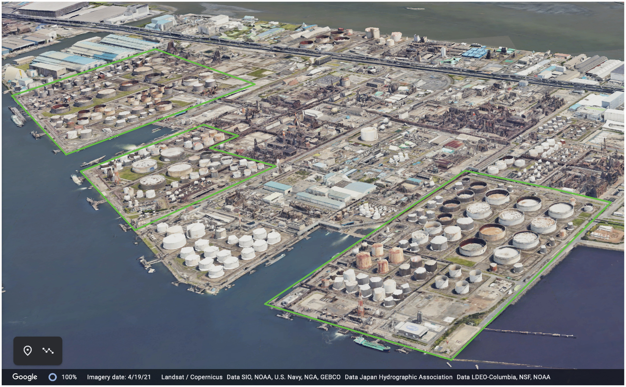
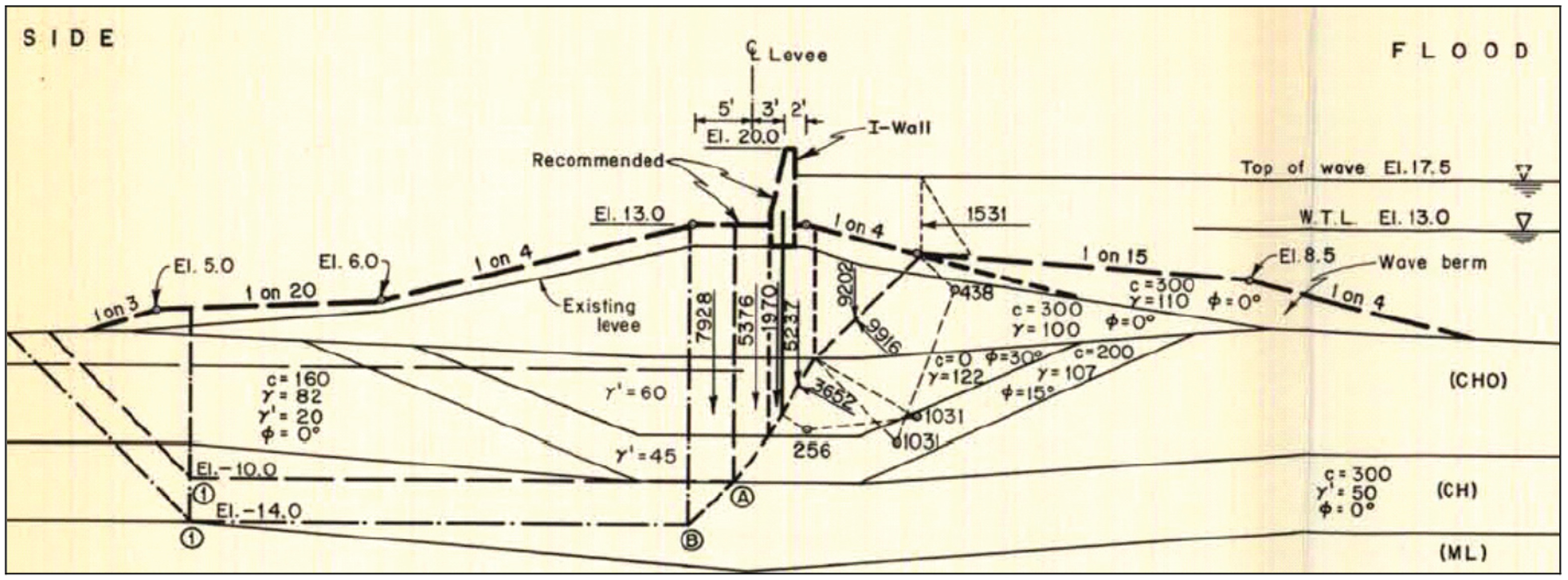
The project involved more than 100 storage tanks founded on loose sandy bay fill in a seismically active harbor (Fig. 1). To protect against offsite loss of product, the facilities were subdivided by firewalls into patios and those patios were contained within larger revetments. Many of the patios were interconnected by underground drainage systems. While the direct cost of foundation failures could be large, they would be exceeded by environmental costs.
Usefulness of Event Trees in Organizing Uncertainties
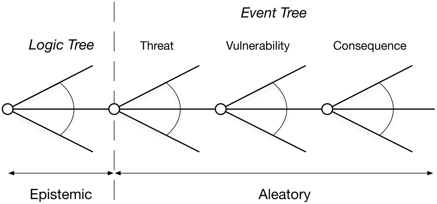
Many of the lessons learned on the Tonen project seem obvious today, but they were less so then. The first was how to build a systems model of the facility. The then-recent WASH-1400 study used fault trees to combine the performances of the many components in a nuclear plant to calculate the probability of accident sequences. A fault tree is a logic diagram that reasons backward from an adverse performance to the faults necessary to cause it (Modarres 1993). That worked well with mechanical-electrical systems that could be fully enumerated. Yet, that was not the case for the tank farm which was a more open system. The tank farm had some components that could be discretely enumerated, like the tanks themselves and drainage pipes and firewalls, but the performance also depended on soil deposits under the site, some natural and some manmade. It also depended on external hazards, specifically earthquakes, that at the time had not been part of the WASH-1400 analysis. Event tree models were used because they were flexible and could be used to combine uncertainties of many types, including those based on judgment (Fig. 2). An event tree is a logic diagram complementary to a fault tree that reasons forward from an initiating event to subsequent adverse performance.

Event trees have since become the standard representation for uncertainties in almost all dam and levee safety studies (Hartford and Baecher 2004; FEMA 2015). They are widely used in offshore applications (Rausand and Haugen 2020) and in mining (Brown 2012). In an event tree, the many uncertainties entering an analysis are laid out graphically, with each node in the tree representing the probability distribution of an uncertainty. The probability of proceeding down a chain of uncertain outcomes through the tree is calculated by multiplying the successive conditional probabilities at each node
(1)
In which = joint probability of the events along an individual path through the event tree from its beginning to an outcome; and = individual uncertainties in the tree. The vertical line indicates a conditional probability of the uncertainty on the left given the occurrence of the uncertainties on the right. The sum or integral of the uncertainties at each node must equal 1.0 because each node is a probability distribution of an uncertainty. Commercial software applications are widely available to do these calculations.
A Taxonomy of Uncertainty for Geotechnical Data
Most of the subsurface data for the Tonen project came from standard penetration tests, which were highly variable (Fig. 3). The geometry of the soil strata differed systematically across the site, so a set of soil models was created. Yegian and Whitman (1978) recently developed a reliability model for relating blow count data to the probability of liquefaction triggering, and that was the approach used. Since the late 1970s, there has been a great deal of work on liquefaction triggering and residual strength, but that came later and is tangential to the present discussion (NRC 2016).
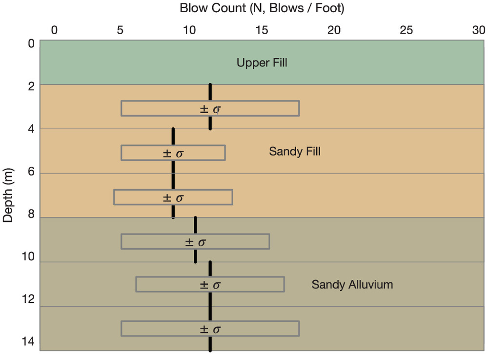
The question arose as to what the large scatter in the in situ data meant for engineering predictions. Some of that scatter was presumably due to real variability and some due to random testing errors. However, in interpreting the data one also had to consider systematic biases in the measurements and biases due to statistical and testing errors. Not each of these errors affects prediction uncertainty in the same way. Spatial variation and measurement noise to some extent average out, but statistical errors and measurement bias create systematic errors that do not. The latter are more concerning because they create correlations of error among the predictions of performance.
A simple taxonomy was developed (Fig. 4), which has later used on other projects (Christian et al. 1994; Baecher and Ladd 1997), in which the variance of the uncertainty in an engineering parameter is approximated as
(2)
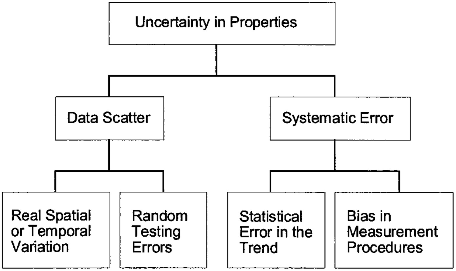
The total variance is the sum of the variance seen in the data plus that of the systematic errors due to small numbers of measurements and measurement error
(3)
(4)
The last of these are now referred to as transfer errors. Variants of this taxonomy have been proposed by Phoon and Kulhawy (1999), Jones et al. (2002), and others.
This simple taxonomy leads to several useful insights. The first is that the variability reported as observed in soil engineering data is often quite large, sometimes showing coefficients of variation (standard deviation divided by the mean) of 30% or more. No one doubts that this variability is observed, but is it applicable to reliability calculations? If yes, then the rates of geotechnical failures would be similarly large, but they are not. The explanation is that some of the data scatter is not in the soil itself but due to testing errors. Such errors add noise to the data. This can be ignored if one can estimate how large they are. This is not simple because most soil testing is destructive. The advent of stochastic models of spatial variation in mining geostatistics along with modern statistical methods of estimation to a large degree solved this problem (DeGroot and Baecher 1993). The systematic errors are due to statistical estimation, the physics of testing, and the pedotransfer functions used to translate measurements into engineering parameters (Phoon and Kulhawy 1999). Systematic errors do not appear in the data scatter and are insidious because they do not average over soil volume.
Importance of Autocorrelated Spatial Variation
The second insight was that the performance of geotechnical structures often depends on averages of soil properties over volumes or areas of soil, for example, the total displacement of a volume of soil or the total shear resistance along a landslide slip surface. Obviously, things are never quite so simple. Differential displacements may depend on the difference between the averages in two volumes, and the weakest link in a long levee depends on the weakest section.
The data scatter in test data, in contrast, reflects averages over the small volumes of soil mobilized in a test. The smaller the volume, the greater the variability among the measurements. The variability of the average soil property within a much larger volume would be less than the variability among the small volumes of the standard penetration test data because the variability averages out. The fragilities of the tanks had been correlated to average soil properties through a large empirical survey (Marr et al. 1982). More recent work by Fenton and Griffiths (2008) suggests that the average property beneath a tank may not be the best criterion for fragility. Were the analysis being done today, it might be done differently, but at the time, fragility was correlated to total settlement.
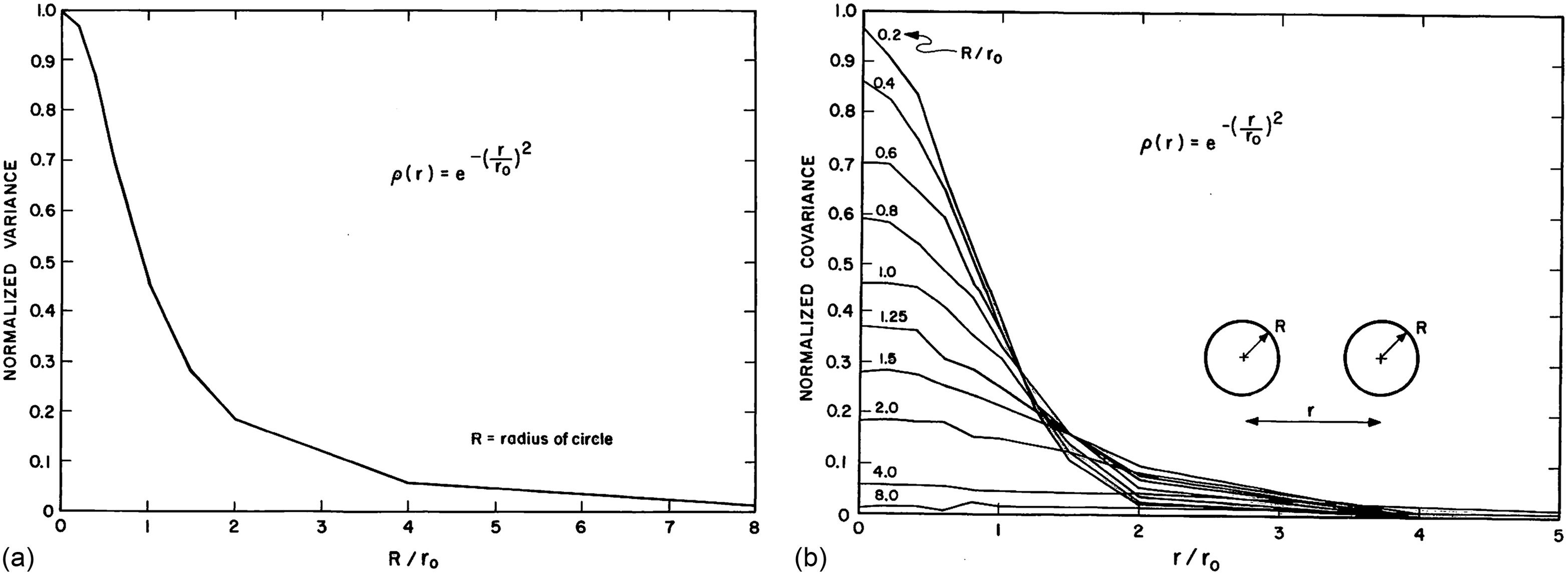
The variance in the average soil properties under a tank depended on the size of the tank. The larger the tank, the smaller the uncertainty in the average soil property (Fig. 5). In this figure, the variances and covariances are normalized to the point variance among test values, and the tank radius and separation distances are normalized to the autocorrelation distance as described in Vanmarcke (1977a).
Additionally, soil properties are spatially correlated. The properties in adjacent volumes of soil tend to be alike and those in distant volumes tend not to be. As a result, the performances of the tank foundations were also correlated. Nearby tanks tend to perform alike. Since the concern was the total volume of product spilled in an earthquake, the total number of tanks failing and the volume of product in each were of importance. The correlations among tanks were important because correlations suggested higher probabilities of multiple tank failures during an earthquake.
Recognition of the importance of spatial correlation of geological properties arose in the mining industry (Krige 1962a, b) but spread quickly to geotechnical engineering with the work of Wu (1974), Vanmarcke (1977a), Høeg and Tang (1978), and others. In recent years, the implications of spatial correlation using numerical modeling have been explored by Fenton and Griffiths (2008).
Communicating Risk to Stakeholders
Among the more useful things learned at Tonen was that communicating risk (probabilities and consequences) to an owner is itself challenging. None of the three earlier Terzaghi Lectures formally defines risk, and their focus is largely on probabilities. The obvious way of communicating risk is by multiplying probability and consequence to get an expected value. One sometimes sees this as a formal definition of risk, but in the field of risk science, the concept is more complex (Kaplan and Garrick 1981). In principle, one ought to be willing to pay up to this expectation to eliminate the risk, but this can be a difficult proposition for the owner.
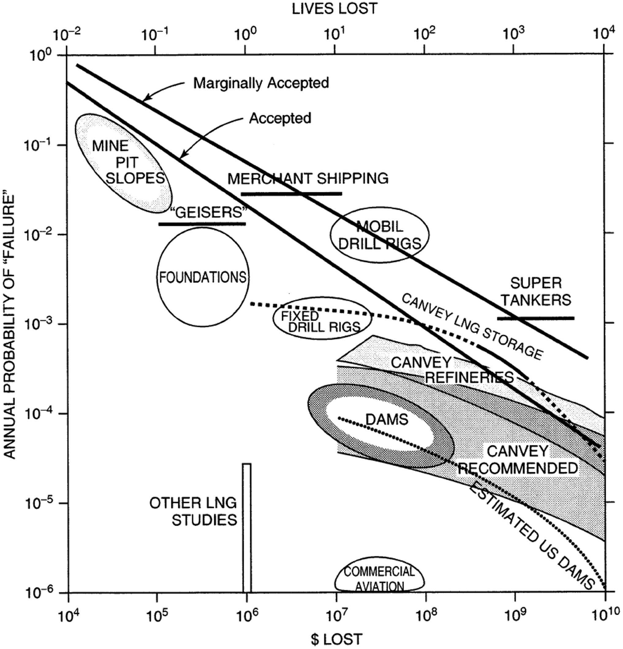
Instead, data were collected on comparative risks for similar facilities and used to compare site-specific risks (Fig. 6). The concept was that this comparative information could be used with regulatory authorities to demonstrate good faith in taking actions to reduce risk. The approach worked well in communicating with the client and in turn with regulators. Whitman published this figure in his Terzaghi Lecture, and it has become well-known. It is fortunate that he did so, because otherwise, it would have quietly disappeared: at the time, no one on the team thought it all that interesting.
Geotechnical Uncertainty I: Probability and Uncertainty
The discussion to this point has dealt with modeling geotechnical uncertainty; however, the Tonen project also led to conceptual insights which took longer to be recognized. These are likely of more consequence than the modeling tools themselves.
Probability Is in the Model, Not in the Ground
Georges Matheron, the founder of geostatistics said, “probability is in the model, not in the ground” (Matheron 1989). There is nothing random about in situ soil properties: they are what they are, but we just do not know what they are. In modern risk and reliability modeling, uncertainties are commonly divided between aleatory and epistemic. Aleatory uncertainties are those modeled as variability (or randomness as in the toss of a coin) in nature and describable by frequencies. Thus, one may model the spatial variations of soil properties across a site as aleatory, but not the properties at a particular point. Epistemic uncertainties are those due to a lack of knowledge and are described by degrees-of-belief. Soil properties at a particular point are unique although possibly uncertain. They may be unknown but are not variable and not describable by frequency. A tradeoff between how much of the spatial variation is modeled as aleatory and how much as epistemic can be made by changing the granularity of the trend model. This is conceptually similar to changing the flexibility of a regression model.
The separation of uncertainty between aleatory and epistemic is mostly a convenience of modeling (Faber 2005; Kiureghian and Ditlevsen 2009). Thus, while it is sometimes said that epistemic uncertainty is reducible (with more knowledge) but aleatory uncertainty is not, that is at most true within the context of a set of modeling assumptions (Vrouwenvelder 2003). For example, it is common in probabilistic seismic hazard analysis to presume that earthquakes occur randomly and independently within the constraints of a source model. In fact, the geomechanics controlling the occurrence and size of the earthquakes are likely deterministic, but we do not know enough to characterize the process as such, so we model the uncertainty as aleatory. That is a modeling choice.
Geotechnical Uncertainties Are (Mostly) Epistemic
Geotechnical uncertainties are mostly epistemic. They have to do with what we know, not about randomness in nature. As a result, they are almost always subjective. The probability theory appropriate to these sorts of uncertainty has to do with degrees-of-belief, not with frequencies (Vick 2002). The lectures of Casagrande, Whitman, and Christian call out the importance of judgment in geotechnical practice, which is simply another name for the subjectivity of most geotechnical uncertainties.
Interagency Performance Evaluation Taskforce
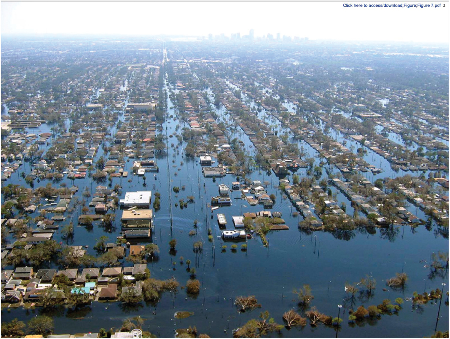
The second project was the IPET (2005–2009). The IPET was organized under the Corps of Engineers to understand the performance of the hurricane protection system in New Orleans during Hurricane Katrina (Link and Harris 2007). This, too, involved risk analysis, but now of an even larger geoengineered system. This system in addition, however, protected human life (Figs. 7 and 8). The system was subsequently renamed, the Hurricane and Storm Damage Risk Reduction System (HSDRRS).
The Risk and Reliability Team initially involved 37 engineers and scientists, of whom six remained active throughout the effort [IPET8 (USACE 2008)]. As at Tonen, event tree models formed the basis of the approach, and the same taxonomy of soil property uncertainties informed the data analysis. Spatial variation again was an important factor, helping to explain length effects in the long levee reaches using the method of Vanmarcke (1977b). Important new lessons from IPET (USACE 2009) included:
1.
The use of logic trees to differentiate the effects of epistemic versus aleatory uncertainty,
2.
Appreciation for the care needed in putting numbers on engineering judgment,
3.
The need sometimes to incorporate legacy data and analyses in risk models, and
4.
Approaches for communicating risk to the public.
Given how IPET was structured, it made sense again, as at Tonen, to divide the risk analysis into three parts (Fig. 9): (1) the threat or hazard, in this case surge, wave, and flood; (2) the vulnerability of the engineered system to the threat (in this case, the hydraulic and geotechnical reliability of the infrastructure); and (3) potential consequences (in this case including loss of life). In other contexts, e.g., homeland security, this has been called the threat-vulnerability-consequence (TVC) approach (NRC 2010a).
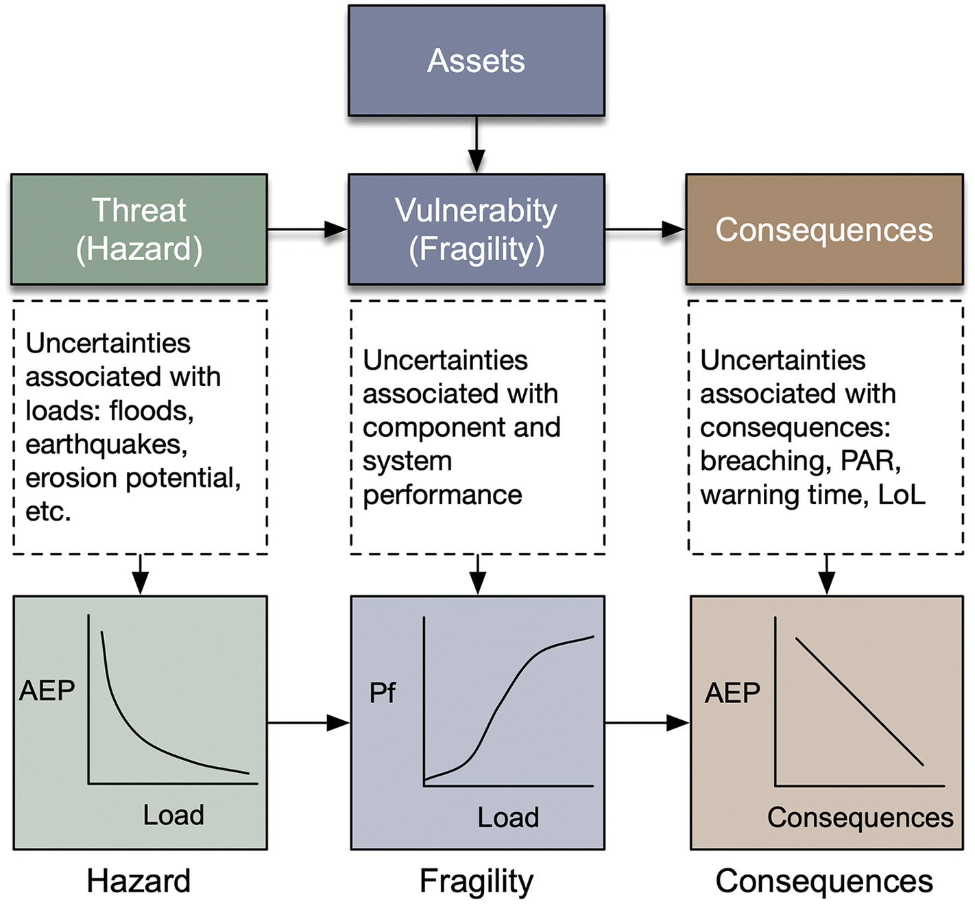
TVC Approach
The TVC approach is widely used for natural hazards. Threats to the system are characterized by probabilities of load levels. These might be surge or flood elevations, peak ground accelerations, wind speeds, malicious intent, or the like. The performance of the system under these loads is characterized by fragility, which is the probability of adverse performance conditioned on load
(5)
The probability of adverse performance as a function of load is commonly called a fragility curve. The probability of the load is combined with the fragility to generate probabilities of adverse performance. Consequences are then associated with adverse performance
(6)
The consequences of IPET included economic loss and potential loss of life, and both of which were uncertain.
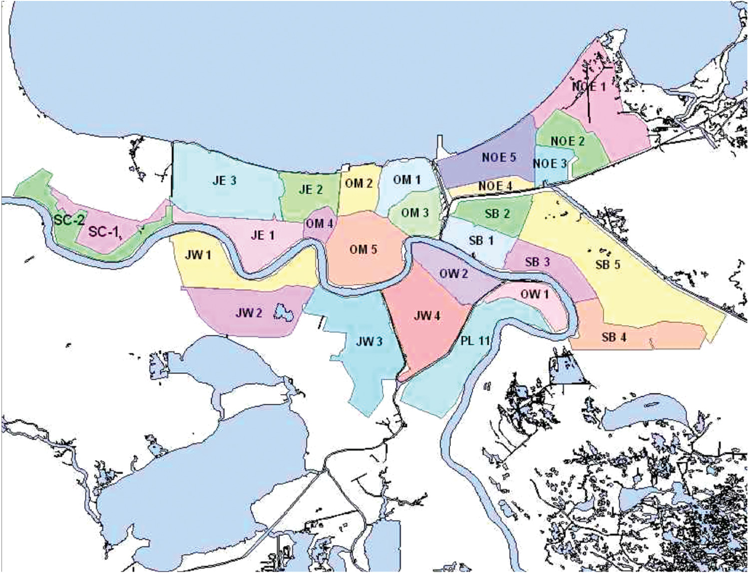
The preHurricane Katrina protection system of New Orleans extended 350 miles. This perimeter was divided into 135 reaches and 197 structural point features. A reach was defined as a continuous length of levee or wall exhibiting homogeneity of construction, geotechnical conditions, hydrologic and hydraulic loading conditions, consequences of failure, and possibly other features relevant to performance and risk. A point feature was defined as a structural transition, gate, pump station, drainage control structure, or other local discontinuity. A portion of the system definition near Lakefront Airport in New Orleans East is shown in Fig. 10 (USACE 2008). This offered the opportunity to examine risk at the census block level or aggregated to subbasins, basins (parishes), or system-wide levels.

The frequencies of occurrence of surge and waves differ around the HSDRRS. The IPET Hurricane Hazard Team developed new statistical techniques based on numerical surge and wave models to quantify these hazards. The model of hurricane occurrence used a joint probability distribution of principal hurricane parameters to characterize the frequencies of storm events based on historical storms in the Gulf of Mexico. An ensemble of about 2000 possible hurricane tracks and characteristics (Fig. 11) was assembled and combined with respect to individual storm probabilities to generate hydrographs at individual reaches or point features around the protection system (Fig. 12) (USACE 2009). This was judged to represent the range of storms that might strike New Orleans and was used to generate the local threat at each reach expressed as the annual probability of surge height.


Fragility Curves
Geotechnical reliability was described by fragility curves that characterized the predicted performance of individual reaches or structures as a function of surge and wave levels. The fragility curves were generated from an evaluation of subsurface conditions, the character of the structures, and relevant failure mechanisms defined previously by the IPET Performance Analysis Team.
There was neither time nor resources to reanalyze the many reaches and features. On the other hand, the New Orleans District US Army Corps of Engineers (USACE) maintained comprehensive historical design records and drawings, with some extending to the creation of the District in 1803 (Fig. 13). These were used to approximate fragility curves for individual reaches based on heritage data and engineering designs, often based on practical but robust methods such as first-order second-moment reliability (Duncan 2000) or expert opinion. This provided what the team judged to be reasonable fragility curves in a timely way, but obviously with less fidelity than a comprehensive reanalysis might have provided using a more modern analytical tool, which in any case was not practicable.
Failure was defined as breaching, which allowed water to enter a protected polder. This failure occurred in two ways: (1) loss of levee or wall stability, or (2) overtopping causing the protected side of the levee or wall to erode and breach (USACE 2007a, b; see Table 1). The loading at which failure occurs varies along the reach and is not precisely known. Part of the uncertainty is due to epistemic uncertainty in the average soil strength or average permeability along the reach, but another part is due to spatial variability within the reach that was modeled as an aleatory uncertainty. The spatial variability also leads to length effects, by which longer reaches have a higher probability of failing somewhere than shorter reaches.
| Failure mode | Hazard | Models and parameters | Source of inputs | Principal uncertainty |
|---|---|---|---|---|
| Static instability | Still-water surge, weak foundation soil’s | Limiting equilibrium stability | IPET5, soil test data, design memoranda, in situ surveys | Soil properties, still-water levels, existing elevations, geotechnical model |
| Under seepage | Still-water surge, high permeability soil’s | Flown at calculations, limiting equilibrium stability | IPET5, soil test data, design memoranda, in situ surveys | Soil properties, still-water levels, existing elevations, geological profile geometry |
| Still-water overtopping and scour | Still-water surge, erodible fill | Empirical correlations from post Hurricane Katrina data | IPET5 | Still-water levels, soil fill properties, existing elevations, scour model |
| Transition point feature erosion | Still-water surge, erodible fill | Empirical observations during Hurricane Katrina | IPET5 | Still-water levels, soil fill properties, existing elevations, scour model |
| Wave runup | Wave heights and periods, erodible fill | Empirical correlations and model test results | IPET4 | Wave height and period, still-water levels, existing elevations |
Failures that lead to a breach of the drainage basin perimeters were associated with four principal failure modes: (1) levee or levee foundation failure, (2) floodwall or floodwall foundation failure, (3) levee or floodwall erosion caused by overtopping and wave runup, and (4) failure modes associated with point features such as transitions, junctions, and closures. The performance team concluded that essentially no failures in the HPS originated in structural failure of the I-wall or T-wall components. The documented failures at I-wall and T-wall locations were almost all geotechnical, with structural damage then resulting.
Four categories of engineering uncertainty were included in the reliability analysis: (1) geological and geotechnical uncertainties involving the spatial distribution of soils and soil properties within and beneath the reaches; (2) engineering mechanics uncertainties, involving the performance of manmade systems such as levees, floodwalls, and point features such as drainage pipes; and the engineering modeling of that performance, including geotechnical performance modeling; (3) erosion uncertainties, involving the performance of levees and fills around floodwalls during overtopping, and at points of transition between levees and floodwall, in some cases leading to loss of grade or loss of support, and consequently to breaching; and (4) mechanical equipment uncertainties, including gates, pumps, and other operating systems, and human operator factors affecting the performance of mechanical equipment.
Logic Trees
An event tree approach was used on IPET (Fig. 14), as at Tonen, but now incorporating logic trees to simplify the separation of epistemic from aleatory uncertainties (Bommer and Scherbaum 2008; Bommer 2012). The idea of logic trees is to separate out the epistemic uncertainties due to lack of knowledge into their own tree and then to condition an event tree containing only aleatory uncertainties on the respective branches of that epistemic logic tree (Fig. 15). This greatly simplifies the event tree calculations by implicitly capturing the correlation structure among the aleatory events, which in the Tonen project had to be manually calculated and entered into the tree, an approach that may also overlook subtle correlations. The logic tree approach had the benefit of separating those uncertainties that can be reduced by collecting more data or improving models from those that cannot (Kiureghian and Ditlevsen 2009).

In hindsight, using event trees was not the best approach. The number of end-nodes in the event trees was in the millions for each of the 76 storm scenarios used in the analysis. This caused computation problems, reduced the number of scenarios that could be computed, and precluded interim results from being easily extracted. Direct simulation using Monte Carlo might have been more powerful and cost-effective. In this case, a nested simulation approach could have been used in which a simulation containing only the aleatory uncertainties is nested within an outer simulation containing the epistemic uncertainties, as discussed below.
Putting Numbers on Engineering Judgment
The subjective probabilities of experts were critical to the analysis. Geotechnical engineers are true believers in the value of engineering judgment to fill in for gaps in information or inadequacies of modeling and analysis. Peck (1980) famously championed this view. Yet human judgment is flawed, and a host of cognitive biases are recognized as affecting how and how well people put numbers on their subjective uncertainty (Baecher 2019; Marr 2019, 2020; Vick 2002).
Communicating Risk to the Public
Consequence data (property and life loss) were generated for each storm scenario. The risk model generated probabilistic estimates of the extent and depth of inundation in each of the 27 polders. Inundation depths were used to interpolate property and life loss estimates for prehurricane Katrina conditions and post 2007 reconstruction conditions. Again, these were portrayed on probability-consequence charts, sometimes referred to today as frequency-number (FN) charts (Fig. 16). The FN chart is a modern formalization of the concept behind Fig. 6. Here, it displays annual exceedance probabilities of risk to life for the preHurricane Katrina and postreconstruction conditions. Similar results from the California Delta Risk Management Strategy (URS 2009) are shown for comparison. The latter results tail off more quickly because the population at risk is smaller.
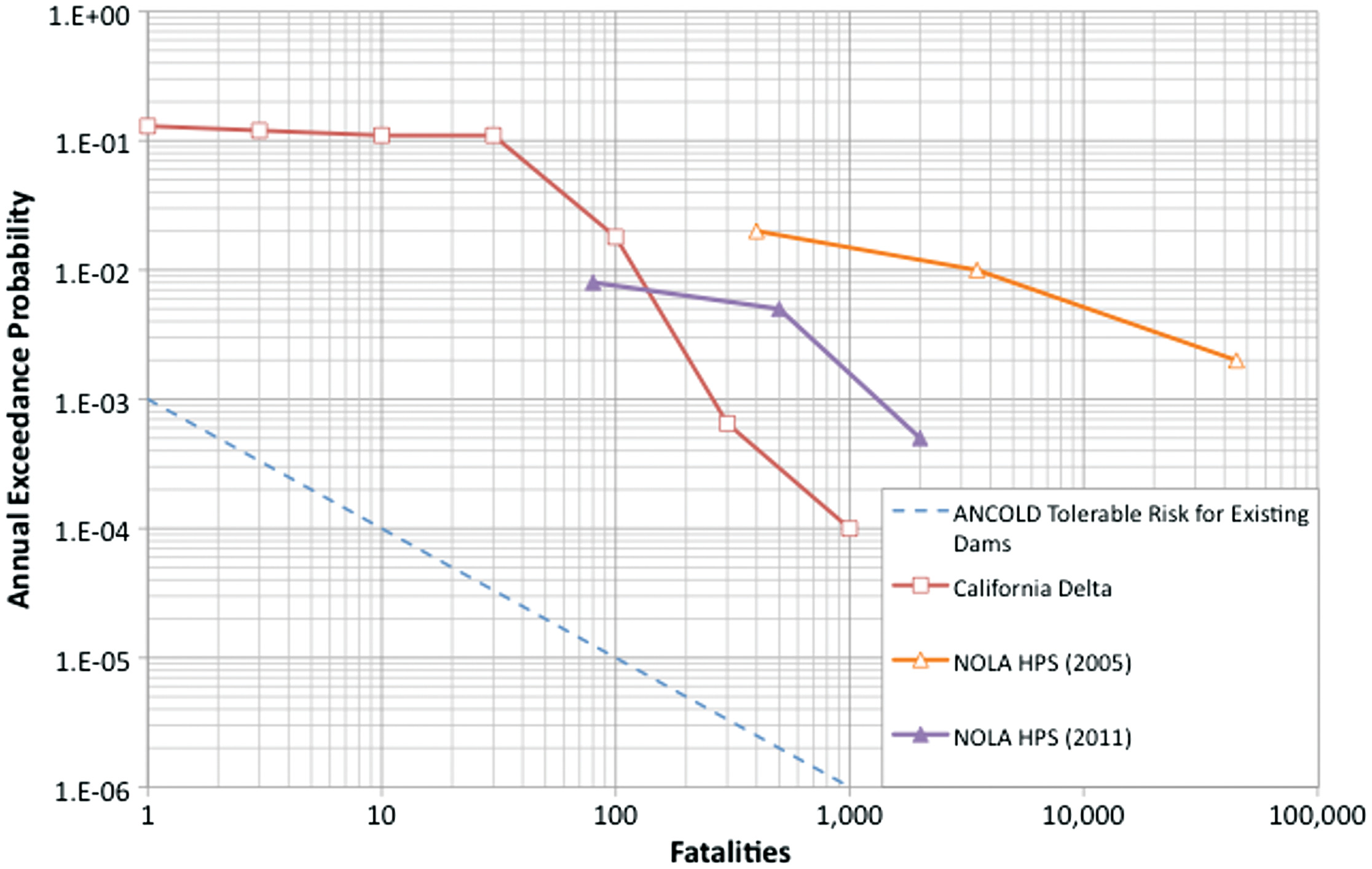
In recent years, the use of FN charts has become common in dam safety (ANCOLD 2003; FEMA 2015), industrial risk (Jongejan 2008), and offshore engineering (Lacasse et al. 2019), among other fields. Criteria for tolerable societal risk have been set by various organizations. Following recommendations by the Australian-New Zealand Committee on Large Dams (ANCOLD 2003) and others, these FN charts have sometimes been adopted as guidelines for tolerable risk, although some organizations such as the Bureau of Reclamation explicitly do not use them for that purpose (Reclamation 2011). These guidelines are typically orders of magnitude lower than the risks existing along the Gulf coast or in riverine flood hazard areas elsewhere in the United States (Fig. 16). Riverine and coastal flood criteria in the United States have historically used a 1% annual exceedance probability as a criterion for insurance and risk mitigation.
Geotechnical Uncertainty II: Bayesian Thinking
The statistics course many of us took in college is mostly useless for geotechnical practice—in the author’s opinion. That course likely focused on a peculiar branch of statistics called, frequentism. There is nothing incorrect with that sort of statistics, but it does not apply to most uncertainties geotechnical engineers face. Frequentist statistics has to do with aleatory variations of the sort found in gambling, medical trials, or the national census. In contrast, geotechnical practice deals mostly with epistemic uncertainties, many involving subjective judgment. Geotechnical practice involves predictions that are usually based on probabilistic characterizations of uncertainties in states of nature, which are not admissible in frequentist statistics. Dealing probabilistically with uncertainties in states of nature requires a degree-of-belief (i.e., Bayesian) definition of probability because of this inadmissibility.
Uncertainty about States of Nature
Two characteristics of Bayesian statistics make it fit for geotechnical use: it allows probabilities to be defined on states of nature such as site conditions or engineering parameters, and it admits subjective probabilities. Frequentist statistics allows neither. Frequentist and degree-of-belief statistics are not in conflict, they are just different. They use the same mathematical theory of probability (Kolmogorov 1950) but differ in ways of defining uncertainty (Baecher 2017). The distinction is philosophical but important because it dictates how one draws inferences and makes decisions.
The distinction is illustrated in Fig. 17. A program of site characterization results in observed data on soil engineering properties, the geometry of the subsurface, or other states of nature to be used in analysis and design. Frequentist statistics treats these states of nature as deterministic but unknown: in that theory, it is meaningless to define probabilities on states of nature because those states do not have frequencies. In frequentist statistics, it is the data that are assigned probabilities, not the states of nature. Inferences are described as confidence bounds, -values, and the like. These characterize probabilities on what data might have been observed, not on the states of nature (Diaconis and Skyrms 2018; O’Hagan 2004). These are direct probabilities.

In contrast, Bayesian statistics takes the data as known (i.e., they have been observed) and calculates probabilities on the states of nature that might have generated those data. Because probability is interpreted as a degree-of-belief and not as a frequency, this is acceptable. These are inverse probabilities (Dale 1999). This is neither new nor unintuitive to geoprofessionals, and most of us are unwittingly Bayesians. de Mello (1975, 1977) was among the first to champion Bayesian ideas, although many others followed (Contreras 2020; Feng 2015; Gambino and Gilbert 1999; Garbulewski et al. 2009; Jiang et al. 2018, 2020; Juang and Zhang 2017; Kelly and Huang 2015; Papaioannou and Straub 2017; Phoon 2020; Schweckendiek 2014; Zhou et al. 2021).
Updating Probabilities
Little is known about the eponymous Rev. Thomas Bayes (1701?–61) (Dale 2003). Even his likeness, which is pervasive in print and on the web, is thought not to be him (IMS 1988). The person to whom we owe the modern and more complete derivation of the theorem is Laplace (1749–1827). In the 20th century, the geophysicist Sir Harold Jeffreys (1891–1989) produced a long treatise on the inverse probability that remains in print today. This way of thinking has a firm geoscience pedigree.
A simple modern representation of Bayes’ Theorem isin which, = some hypothesis (which could have to do with an event, a probability distribution, or anything else about which one is trying to learn; = prior probability of the hypothesis; = posterior probability of the hypothesis, given the observed data; = Likelihood of hypothesis based on the data (i.e., the conditional probability of the data were the hypothesis true); and = marginal probability of the data irrespective of (a normalizing constant).
(7)
The marginal probability of the data is readily found from the total probability theorem as the weighted sum of the probability of the data under the two respective hypothesesin which = complement, i.e., “not-H.” In more complicated applications, the normalizing constant is often determined numerically.
(8)
Perhaps the simplest example is the well-studied question of whether some geological detail exists at a site although undetected in exploration (Christian 2004). Presume that one believes that the probability of such a detail exiting at the site before exploration is performed was . This might be a subjective judgment or might be based on geological information. Perhaps a geophysical survey has been undertaken with a chance of finding an existing target of the given description, but it fails to find anything. The probability of the target existing undetected after exploration can be logically updated using Eq. (7) to bein which, = geological detail exists; = geological detail does not exist; Data = geological detail not found in exploration; = prior probability geological detail exists; = posterior probability geological detail exists, given that it was not found; = conditional probability of not finding the geological detail if it actually exists. There are many things to be learned from this seemingly simple equation:
(9)
1.
First, data never speak for themselves. They only tell us how to update from a prior probability (what we thought before seeing the data) to a posterior probability (what we should logically think afterward). Lindley (1985) said, “today’s posterior is tomorrow’s prior.”
2.
Second, updating probabilities from priors to posterior is a straightforward matter of multiplying the prior by the weight of evidence in the data. The weight of evidence is entirely contained in this conditional probability of the data given the hypothesis. The term of art for this conditional probability is the likelihood.
3.
Third, at some point in history there are no data upon which to base a prior; therefore, the priors are ultimately a matter of judgment and necessarily subjective.
4.
Fourth, this is the mathematics of learning by experience. It is the logic of Terzaghi’s (1961) observational approach.
Typically, the prior probability distributions in the Bayesian equation are updated by site characterization, construction, and performance data. The messiness of the mathematics of doing this updating through complicated engineering models for a long time impeded practical applications; however, the advent of numerical methods like Markov chain Monte Carlo (MCMC) has facilitated practical use (Robert and Casella 2010).
Terzaghi proposed the “learn-as-you-go” approach. Peck (1969) gave it the name, observational method. It is now an essential feature of geotechnical practice. The environmental community calls it, adaptive management. Einstein (1991) and Wu (2011) developed a quantitative Bayesian approach to the observational method, as de Mello (1975) had also suggested.
Site Characterization and Sampling
The uncertainties of site characterization and their probabilities are inverse probabilities. They are probabilities defined on states of nature, not probabilities on the data which are observed from those states. Hoek (1999) in the 2nd Glossop Lecture commented that a geological model—conceptual, hand-drawn, or computer rendered—is the building block upon which the design of any major construction project is based. It is principally the geological model that generates the prior probabilities in Eq. (7). A recent example of the importance of the geological model in interpreting the statistics of deep-driven pile performance is provided by McGillivray and Baecher (2021).
One reads that site characterization is so uncertain because we sample but a small fraction of the subsurface. This ignores statistical science. Political polls in US elections sample but a tiny fraction of the electorate, maybe 1,000 out of the 100 million who vote nationally, or about 0.001% (FiveThirtyEight 2022). The inferential uncertainty in sampling does not relate to the fraction sampled but to the number. A more dangerous error is what Tversky and Kahneman (1971) call the law of small numbers. Most of us intuitively presume that the law of large numbers (that the properties of a sample asymptotically approach those of the universe from which they are taken as the sample size becomes large) applies to small samples as well—which of course it does not. If we take a handful of measurements, one is often surprised that the following measurement is quite different from those already observed. One should not be, it just reflects the variability within small samples.
An additional concern—mostly ignored—is whether a sample of measurements is chosen randomly. This is almost never the case in site characterization. Almost always the locations of sampling are what statisticians call purposive. That means the locations are chosen on purpose for one of many reasons: spatial coverage, least favorable places, or places that have the most influence on design. In any event, a purposive sample is not a random sample. Why does random sampling matter? It matters because the presumption of all statistical methods is that the data are random. If they are not random, then the statistical theory does not apply. The infamous Literary Digest poll in the 1932 election between Landon and Roosevelt is a painful example (Lusinchi 2012). It predicted a Landon victory, while in the event, Landon won only Vermont and Maine. The nonrandom sample was taken from the magazine’s subscribers who were mostly wealthy.
Judgment versus Statistical Methods
Casagrande avoided quantitative probabilities as did most of his contemporaries, choosing verbal descriptions such as “grave risk” and “great uncertainties” instead. We know today that verbal descriptions can be deceiving (Baecher 2019), and psychological research has demonstrated that intuition is a poor substitute for the laws of probability when evaluating uncertainty. Experts are systematically overconfident in reporting uncertainty, ignore base rates (i.e., prior probabilities), disregard the variability of small samples, believe in the Prosecutor’s Fallacy of reversed conditionals (Aitken and Taroni 2004), and exhibit many other systematic errors in reasoning about probabilities. These can all be dealt with but need to be understood.
In a long set of experiments in the social sciences and medicine, the American psychiatrist Paul Meehl (1954) and later the psychologist Robyn Dawes (Dawes et al. 1989) demonstrated that even simple statistical models like regression analysis significantly outperform clinical judgments. This was a precursor to the later work of Tversky and Kahneman. Recently, Morgenstern (2018) has made a related suggestion concerning dam safety and risk, specifically in the relationship between empirically-driven and purely subjective appraisals: “Whether precautionary or performance-based, or even utilizing subjective judgments based on experience, it is essential that the risk assessment process be constrained by evidence and its evaluation to a higher degree than is currently the case.”
Panama Canal Natural and Chronic Risk
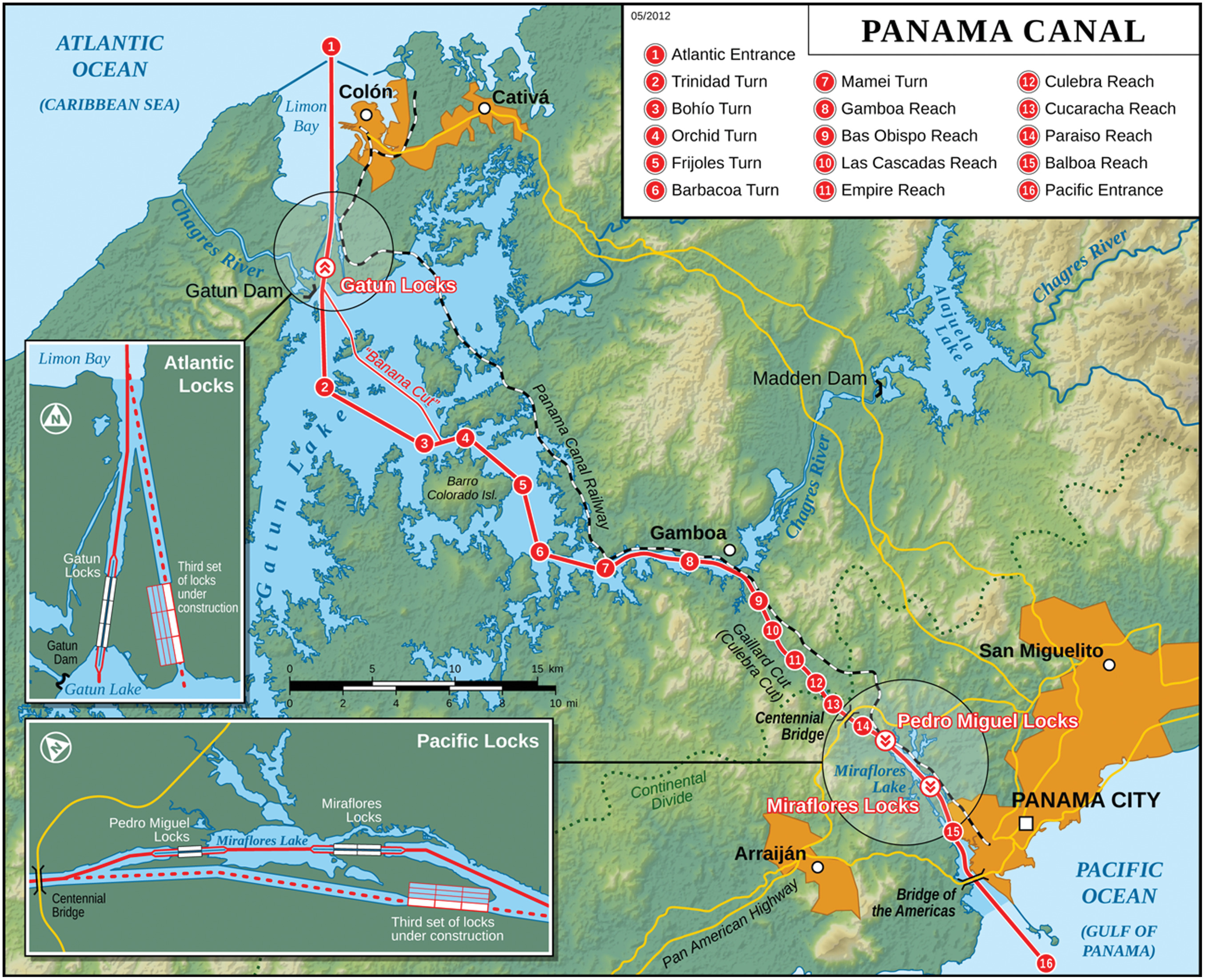
The third project was the natural and chronic risk study—an enterprise risk analysis—for the Panama Canal Authority (ACP) (2011–2016), an attempt to quantify enterprise risk. The Panama Canal, commissioned in 1914, is among the world’s iconic engineering achievements (Fig. 18). The Canal transits 14,000 vessels a year carrying more than three percent of world maritime trade. In the early 1900s, the Panama site was thought free of natural hazards and therefore favored over other crossings. History has changed that appraisal, and it is now understood that seismic, hydrologic, and meteorological hazards all affect the Canal. In addition, an engineered system of this scope faces chronic risks due to operations, aging, and maintenance.
Important new lessons from the ACP project included (Alfaro et al. 2015)
1.
The power of qualitative risk appraisal to organize a systems risk assessment,
2.
The power of effective risk communication with management, and
3.
The usefulness of scenario risk assessments.
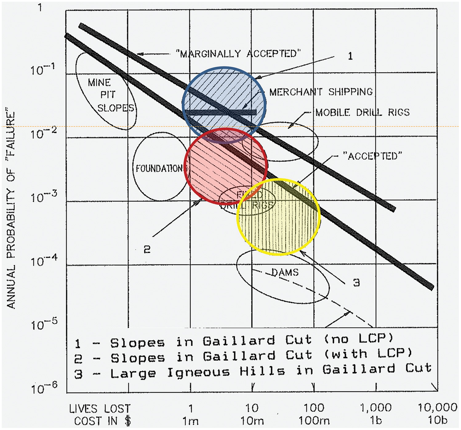
The Engineering Division of ACP had long used risk-informed thinking. An early example was its use of FN curves for communicating to management risks involved with its slope instrumentation program for the Gaillard Cut (Fig. 19). This was but a few years after Whitman’s Terzaghi Lecture. The chart was used to communicate what the impact of a landslide control program could be on risks faced by the Authority and thus to justify a significant investment.
The natural and chronic risk assessment began with a qualitative risk register. The risk register categorized risks by type of asset at the Canal (dams, locks, cuts, gates, power stations, water plants, and others) and among various hazards (seismic, hydrologic, meteorological, operational). The annual risks across the various asset types and failure modes were compiled. Given the magnitude of these risks, management considered two questions: (1) is a particular risk acceptable, and if not, and (2) how much must it be reduced or how can it be managed? FN curves were used as a qualitative means of making these judgments.
Scientific and operations data were compiled to characterize risk, while reliability models were developed to translate those data into actionable assessments. Risks were categorized as catastrophic, significant, or moderate. The first set was modeled in detail; the others were managed operationally. The resulting probabilities and consequences were tracked to understand where risk remediation was called for. This comprehensive risk assessment allowed ACP to reduce risk while controlling costs.
Qualitative Risk
Beginning in 2011, a qualitative risk analysis was undertaken. The project was divided into phases. The initial phase was the development of a risk register. The risk register is a list of threats, facilities, and facility components that might be affected by those threats and possible consequences if those threats occurred (Table 2). The risk register has become a common tool in geotechnical engineering, especially in underground construction. The risk registers at ACP ran to 600 items across all asset classes, but these were reduced to a few dozen highly important risks that were then modeled and analyzed in detail.
| Type | ID | Event | Description | Component | Failure mode | Mode | Failure cause | P | C |
|---|---|---|---|---|---|---|---|---|---|
| DAM | Gatun | Floods | PMF | Crest | Erosion | Erosion | Overtopping | 2 | 1 |
| Upstream slope | Erosion | Erosion | Spillway operation | 1 | 5 | ||||
| Landslide | Landslide | Excess for when the pressure | 3 | 5 | |||||
| Downstream slope | Erosion | Erosion | Over topping | 2 | 1 | ||||
| Landslide | Landslide | Excess pour water pressure | 3 | 5 | |||||
| Landside abutment | Erosion | Erosion | Water infiltration | 3 | 5 | ||||
| Spillway abutment | Erosion | Erosion | Overtopping from the spillway | 1 | 5 | ||||
| Earthquake | MCE | Crest | Erosion | Erosion | Overtopping due to settlement by ground shaking | 2 | 1 | ||
| Upstream slope | Landslide | Landslide | Large deformation due to liquefaction | 2 | 5 | ||||
| Downstream slope | Landslide | Landslide | Large deformation due to liquefaction | 2 | 5 | ||||
| Landside abutment | Deformation | Deformation of section | Settlement or slide due to liquefaction | 3 | 5 | ||||
| Spillway abutment | Deformation | Deformation of section | Settlement or slide due to liquefaction | 3 | 5 | ||||
| Foundation | Piping | — | Loss of material due to liquefaction or hydraulic gradient | 2 | 1 | ||||
| Aging | Surrounding structures | — | Corrosion of outlet pipes and piping | — | — | — | — | ||
| — | Deterioration of penstocks leading to piping, erosion, slides | — | — | — | — | ||||
| — | Deterioration of pipes leading to piping, erosion, slides | — | — | — | — | ||||
| Seiche | Large landslide in lake | Crest | Erosion | Overtopping by waves | Overtopping from large waves | 2 | 1 | ||
| Upstream slope | Landslide | Erosion due to wave action | Erosion due to the cyclic action of waves | 3 | 5 | ||||
| Rapid drawdown | — | Upstream slope | Landslide | Reduction of effective stresses | Impact | 1 | 1 | ||
| Collision | Service barge | Upstream slope | Impact | Impact | Overtopping | 3 | 5 | ||
| Hurricane | — | Crest | Erosion | Overtopping | Excess pour water pressure | 2 | 1 | ||
| — | Downstream slope | Landslide | Excess pore water pressure | 3 | 5 |
Source: Data from Alfaro et al. (2015).
The purpose of the risk register was to identify as many significant risks to the Canal infrastructure as possible and to rank those risks for further analysis. The rank-ordering categorized risks into three sets: (1) those that were thought to require further analysis and possibly modeling to obtain quantitative assessments, (2) those that were significant and needed to be monitored but were thought not deserving of detailed analysis, and (3) those that could be managed as part of normal operations. A qualitative risk rank was used to compare the structures and components within the portfolio. The development of a qualitative risk assessment required many working sessions to develop categories of hazards and an inventory of critical infrastructure. ACP used its own subject matter experts in multidisciplinary teams to assess the likelihoods and consequence and the partitioning and ordering.
In the qualitative phase, simple rankings were assigned to probabilities and consequences. Both the probability of the hazard and the severity of consequence were ordinal-scaled from one to four. This provided a starting point, but ordinal scales suffer many limitations (Stevens 1946). Ratio scales with a true zero and defined intervals were needed for both probability and for consequence (Table 3). An attempt was made to anchor these semiquantitative scales to events and outcomes with which ACP’s subject matter experts were intuitively familiar.
| No. | Verbal description | Example | Value |
|---|---|---|---|
| Probability | |||
| 1 | Very likely | Small landslide, draft restrictions | |
| 2 | Likely | Landslides without controls | to 0.01 |
| 3 | Unlikely | La Purisima 2010 | to 0.001 |
| 4 | Very unlikely | Large earthquake | |
| Consequence | |||
| 1 | Complete loss of navigation operations for more than a year | Loss of Gatun or Madden Dam | |
| 2 | Impede operations for a long period () or create major direct or indirect economic cost | Extensive loss of toll revenue. Seriously compromise the reliability of important components | $1–10b |
| 3 | Impede operations for a short period () or moderate direct or indirect economic cost | Moderate loss of toll revenue. Direct repair costs greater than $500m | $500m-1b |
| 4 | Damages that affect canal capacity and revenues | More than $100 m loss of toll revenue. Direct repair costs greater than $100 m | $100m–500m |
| 5 | Economic damages but the canal continues to operate | Less than $100 m loss of toll revenue. Direct repair costs less than $100 m. No impact on ACP reputation | |
Source: Data from Alfaro et al. (2016).
Quantitative risk analysis was subsequently conducted using the TVC approach. The hazards to which the Canal is exposed were divided into three categories: natural, operational, and malicious. The three most important natural hazards were seismological, hydrological, and geotechnical. A variety of others were considered—hurricanes, tsunamis, tornadoes, and sedimentation—but none led to catastrophic consequences. Operational hazards were those that arise in the operations and maintenance of the Canal and those due to aging. These included navigation incidents, dredging and tug erosion, and time-related deterioration. The historical record of adverse performances and failures suggested that operational risks were significant for noncatastrophic outcomes. Malicious anthropogenic hazards were the subject of a separate study done by a separate branch of ACP.
Risk Communication to Management
The performance of individual components was summarized either as a fragility curve associating a probability of failure with load, leading to discrete failure versus no-failure outcomes; or as a systems response curve, associating a performance indicator with load (e.g., displacement, deformation, factor of safety). The corresponding analyses were made using structural and geotechnical reliability methods adapted to historical data. Consequences were divided into three types: (1) direct cost, (2) lost revenues, and (3) implications for the national economy. Due to the nature of the Canal, the economic impact of adverse outcomes to the nation can in some circumstances be far greater than the direct damages. Only monetary losses were considered.
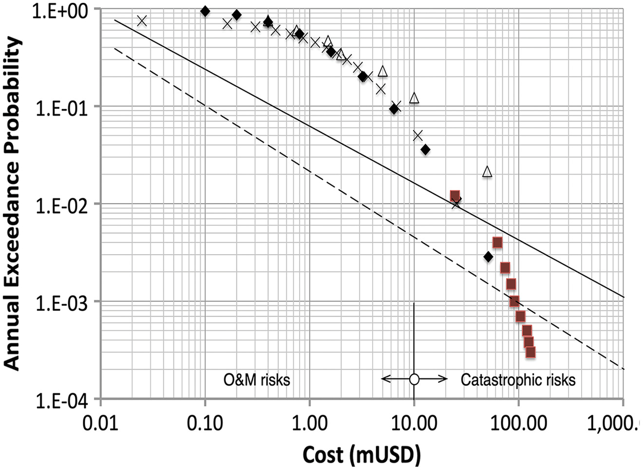
Typical results for slope failures in the Gaillard Cut are shown in Fig. 20. To the left-hand side are historical failures due to rainfall and channel erosion. These are not catastrophic in that they occur nearly every year and are managed by monitoring and maintenance, but they can be expensive. To the right-hand side are low probability-high consequence risks associated with potential earthquakes. These are potentially catastrophic in that long sections of the slope might slide, possibly leading to a temporary closure of the Canal. The decision was made to separate catastrophic from routine risks at a cost of USD 10 m. Although frequent and costly, slope instabilities with consequences smaller than this were considered a necessary and historical cost of doing business.
Scenario Risk
System simulation rather than detailed event trees was used to analyze risks. As had been learned in the IPET project, full-enumeration techniques like event trees become unwieldy for large systems with many components and many uncertainties. Another benefit was also recognized, which was the utility of simulation for modeling and understanding scenarios of risk simultaneously affecting large parts of the system. A large distributed system like the Canal comprises hundreds of assets including water retaining dams and dikes, navigation infrastructure, pumping facilities, electrical generating stations, water treatment plants, and many others. These are mostly interconnected by the hydraulic system of waterways and structures. How does this large number of interacting assets react to a unique natural hazard event—say, a large earthquake—which simultaneously affects them all? An engineering analysis of individual structures or components is clearly of interest, but the adverse performance or failure of one may have cascading effects on others (F. Nadim, personal communication, 2014). For example, the loss of a pool at Madden Dam during an earthquake would have cascading effects downstream at the Pedro Miguel and Miraflores Locks, and the capacities of which might also have been compromised by the same earthquake. There may be nonlinear and even feedback effects within the larger system of assets. These interactions may be obvious in hindsight, but the system simulation may allow their identification ex ante by data mining of simulation results. This has been demonstrated in recent investigations including large-scale dam safety studies on the Göte River system in Sweden (Ascila et al. 2015), the Cheakamus System in British Columbia (King 2020), and the Lower Mattagami River Project in Ontario (Zielinski 2021).
Geotechnical Uncertainty III: Safety
How safe is safe enough? In Panama, the consequences of adverse performance were mostly financial. This is not always the case with geotechnical risks. For example, in dam safety, life safety risk can be significant, and the tradeoff between risk and mitigation is not simply financial. Portrayals of risk in the form of FN curves for this purpose have become increasingly common. Whereas the projects that presented the visualization of risk were descriptive, caution is needed in approaching FN charts as prescriptive. As Petroski (2011) has written, “Safe is not an engineering term;” it is social and political.
FN charts are solid tools for illustrating and comparing risks, but one must be cautious when interpreting them as criteria. In Tonen, IPET, and ACP projects, situations were identified for which risks exceeded common tolerable criteria yet were willingly accepted for rational reasons. At Tonen, the project preceded modern criteria and used benefit-cost thinking. At IPET, the 1%-flood criterion common in US flood protection was legislated by the US Congress. At ACP, the high risk of the Gaillard Cut slopes was deemed a necessary cost of business.
An FN chart for risk-to-life plots the exceedance probability of events leading to a number, , of fatalities. The notion of risk-to-life criteria is sometimes attributed to the British nuclear establishment and the (UK) Health and Safety Executive (HSE 1992a), but careful reading suggests little quantitative guidance from those agencies except on the magnitude of individual risk. HSE (2001) suggests that existing risks to the individual should be on the order of 10−3 per annum for voluntary activities and per annum for involuntary activities. The per annum value is used in much of contemporary dam safety guidance (e.g., ANCOLD 2003). Individual risk pertains to the probability of harm to a single person; societal risk in contrast pertains to the probability of harm to groups of people.
HSE notes, “It is not […] for the regulatory authorities but for Parliament and the public to weigh the benefits of […] the risks we have outlined.” Morgenstern (2018) in his de Mello Lecture makes a similar comment, “The vocabulary of ‘tolerable loss of life’ is provocative and should require stakeholder engagement as well as special risk communication efforts before the criteria become legal regulations.”
The acceptability of risk due to natural hazards and accidents has been approached from many directions. Three are common: (1) revealed preferences, acceptability may be compared to other risks that people appear willing to accept; (2) stated preferences, acceptability may be taken from people’s willingness-to-pay at the margin to reduce risks; and (3) benefit-cost analysis, acceptability may be calculated by balancing monetized benefits including the statistical value of lives saved against monetized costs.
A response within many regulatory agencies is to adopt a value of statistical life (VSL) for inclusion in benefit-cost analysis (Aldy and Viscusi 2003). VSL is the marginal rate of substitution of income or wealth for mortality risk (i.e., for incremental change in risk), usually measured by willing to pay. Geotechnical engineers have been reluctant to adopt VSL for fear of implying a “dollar value of life.” The same has been true in UK practice. This led in the latter instance to a recognition that technological risks are seldom either safe or unsafe, and the concept that if a risk is not so large as to be unacceptable, yet not so small that no further precaution is necessary, then it should be “reduced to the lowest level practicable, bearing in mind the benefits flowing from its acceptance and taking into account the costs of any further reduction” (HSE 1992b). This is the As Low as Reasonably Practicable principle (ALARP).
ALARP seems an eminently reasonable idea, but its difficulties are in its details. One detail is how to evaluate, practicable. Arguments have been made that this is a benefit-cost comparison: what are the benefits of risk reduction and how do they sum relative to the costs of achieving them? That lands us in a circular argument involving VSL. ALARP seems a good idea, but its implementation remains problematic. The same applies to the safety case, which while a reasonable and appealing concept, can be difficult to apply in other than a qualitative way (FEMA 2015).
Spillway Systems Reliability
The fourth project was the Spillway Systems Reliability Project (SSRP) (2000–2016), a joint-industry effort of the large hydropower owners: British Columbia Hydro, Ontario Power Generation, the USACE, and Vattenfall AB. The goal was to consolidate existing knowledge on the reliability of spillway systems, develop an engineering basis for the assessment of safe discharge, establish a methodology for spillway safety assessment, and prepare a systems-based guideline (Hartford et al. 2016). Important lessons from the SSRP involved:
1.
The concept of emergent risk,
2.
Nested simulation, and
3.
Operational safety and human factors.
The project was motivated in part by an observation that the traditional TVC concept of risk might not apply well to spillway reliability. The reason was that the demand on a spillway (the “threat” in TVC) is not a simple load but is a function of the system; it depends on things other than just the maximum reservoir inflow. The traditional demand function mostly ignores operational and system effects, including the interplay of human operators, modern sensors, and control systems. This realization was not an indictment of the risk-based approach but suggested a need to extend risk-based techniques.
Emergent Risk
Many incidents and even failures of geotechnical systems occur not because of simple extreme loadings but because of the interactions of hazards, external disturbances, mechanical and electrical systems, SCADA (supervisory control and data acquisition) systems, and human operators (Nelson 2009; Regan 2010). It is the interactions among these, influenced by organizational factors, training, and management influences, that often contribute to incidents and even failures. This can be seen in the recent Oroville (FERC 2018) and Edenville forensic reports and in National Performance of Dams data (McCann 2008). The importance of such interactions is not unique to geotechnical systems but applies across the spectrum of technological risks (Reason 1997; Leveson 2012).
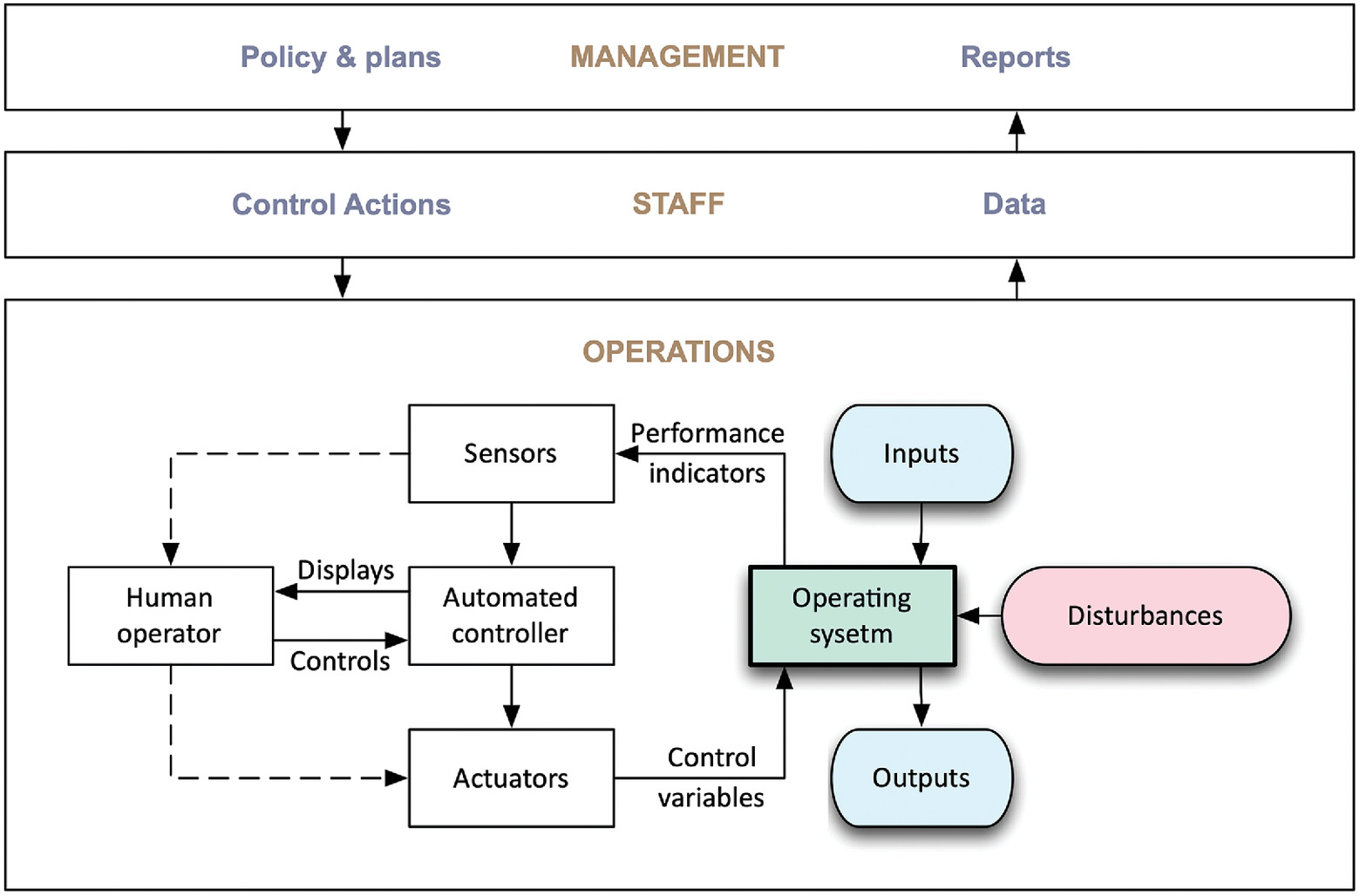
The approach to the analysis and understanding of operational safety starts from the observation that the dominant risks to be managed typically derive not from unique events but from adverse combinations of more usual events. Hartford et al. called these, “unusual combinations of usual conditions.” The timing of such events and their magnitudes can create conditions for which the system had not been designed and which were not accounted for in preparing operational plans. The things that commonly enter a linear probabilistic risk analysis (PRA) are the system inputs, an engineering model, a set of disturbances, and the system outputs (Fig. 21). Disregarded are the many parts of the overall system that also influence safety (Rasmussen 1997; Perrow 2007). The result is that many systems failures do not fit within a simple TVC framework and need to be simulated to identify behaviors that arise out of the interactions among parts of the system. These behaviors are sometimes called “emergent” and are not easily identified ex ante. Decompositional risk analysis tools such as failure-modes and effects analysis, event trees, and fault tree analyses work well in PRA but less well in uncovering systems behaviors.
For many applications in the natural sciences, social sciences, and industry, simulation modeling has become a common tool for analysis and understanding. The use of large-scale stochastic simulation to study complex systems is now common in many scientific disciplines, especially when exploring questions that are poorly suited to traditional reliability analysis. Today, simulation approaches are used in fields as disparate as oil and gas exploration, medicine, materials science, urban planning, and aerospace (NSF 2006). Over the past decade, the US National Research Council has published more than a dozen reports on the use of simulation in engineering science (e.g., NRC 2002, 2008, 2010b).
Nested Simulation
A common way of approaching emergent behavior is by simulation. This might be using a Monte Carlo model, systems dynamics, agent-based models, or one of many other similar approaches (Gianni et al. 2018). Monte Carlo simulation of a rudimentary kind had been used on both Tonen and IPET. On Tonen, it was used to extrapolate the relatively small event trees for individual patios to the larger interactions among the many components of the entire facility. On IPET, it was used to understand length effects on levee reliability and to investigate combinations of failures (e.g., gate openings, levee penetrations, and structural discontinuities).
The simulation approach goes beyond traditional reliability that considers ultimate geotechnical, structural, hydraulic, and other capacities treated separately to one that considers many simultaneous ways that a system can perform adversely (Hartford et al. 2016). There are good reasons for the increasing popularity of simulation in risk analysis: simulation allows complex systems to be modeled easily and cheaply, computer speeds are increasing, discrete events are readily included, interactions among differing types of system response (e.g., physics of failure, communication and control, and human reliability) can be represented, and the numerical precision of simulation is often independent of the complexity of the system being modeled.
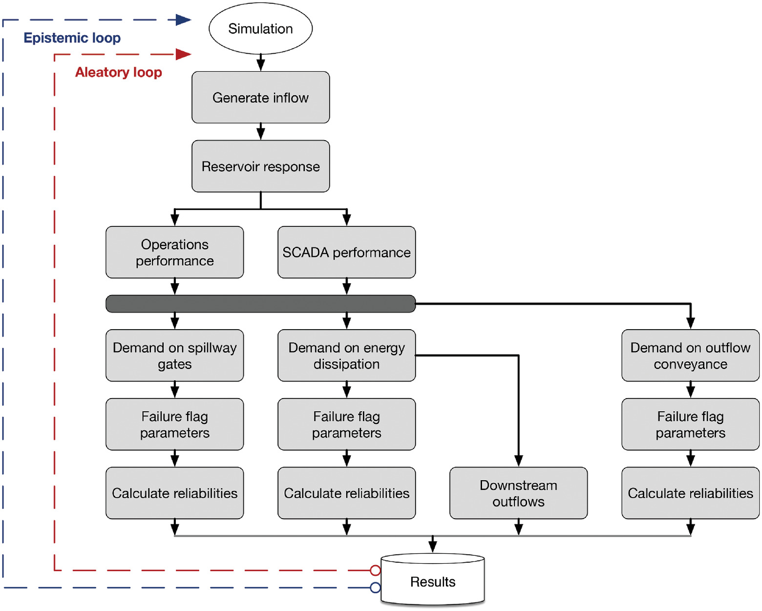
It was observed on IPET and later in Panama that separating epistemic and aleatory uncertainties in event tree analysis by using logic trees was powerful. This allowed model, parameter, and other systematic uncertainties to be separately considered and the possible correlations they generated to be accommodated implicitly. A similar approach is possible with simulation. First, a simulation model is developed containing only the aleatory uncertainties of interest to the problem (Fig. 22). The probabilities of the aleatory uncertainties are taken to be conditional on the values of the epistemic uncertainties. A second simulation loop of just the epistemic uncertainties is nested around the first aleatory loop. For each realization of the uncertainties in the epistemic loop, the aleatory loop is iterated many times. Then, the epidemic loop is itself iterated many times. Finally, the two sets of results are combined. A similar approach was used by USACE in its risk analysis of the Herbert Hoover Dikes (USACE 2014).
Human Factors
A third thing that was learned on the SSRP was the importance of human factors to operational safety. This has been emphasized in recent forensic investigations of dam incidents and failures (FERC 2018, 2022) and has been discussed in specific detail by Alvi (2013). Humans are tasked with making decisions and implementing actions to operate a system in a safe and efficient way. This involves both cognitive and physical responses. Depending on the event sequence, human errors can lead to consequences ranging from minor to the shutdown of a facility or to failure. It is reasonable to incorporate human reliability in systems models as is routinely done in nuclear, oil and gas, and other hazardous industries. This topic is beyond the scope of the present discussion, but increasing attention is being paid to its importance.
Path Forward
Geotechnical practice has come a long way in its use of risk and reliability thinking since Casagrande’s lecture in 1965. What started in the 1970s as relatively simple probabilistic versions of traditional design equations has evolved into risk analyses of large engineered systems, like those used in other engineering disciplines. These methods are now routinely applied to dam safety, large industrial projects, flood and coastal protection projects, offshore facilities, and other large geotechnical works. They are used to inform infrastructure decisions, develop public policies, and ensure public safety.
The earlier Terzaghi Lectures of Casagrande, Whitman, and Christian each call out the importance of evaluated judgment in geotechnical practice. Data may seem objective, but they are always filtered through the lens of geology and experience. The current generation of risk-informed tools that have evolved since those lectures are consistent with that way of thinking, placing it on a coherent conceptual footing.
Nonetheless, challenges remain. Among the most obvious challenges continues to be education. There remains confusion in practice over the nature of probability in geotechnical engineering and the meaning of statements made about uncertainty. Whereas a rudimentary understanding of probability and statistics has become necessary in most technical professions, it has languished in geotechnical engineering. Most practitioners appear to accept the fundamentally subjective character of uncertainty in geotechnical practice, and most apply some form of Bayesian thinking, inverse probability, and observational methods whether or not done so explicitly or even knowingly.
We also face conceptual challenges. One is the increasing nonstationary of natural hazards. Whereas in the past the historical record could be extrapolated to predict the future; in a nonstationary world of climate change, the past may no longer be a prelude. Our forecasts of future hazards increasingly are functions of the epistemic uncertainties of models and scenarios rather than the aleatory uncertainties of the historic record. Risk methodology is up to the task, but new conceptual approaches to design and policy are needed. It seems inevitable that the observational approach, adaptive planning, and Bayesian methods of learning from experience will be a central part of that thinking.
Another challenge is how society judges the tolerability of risk. Today, life and safety risks posed by critical infrastructures vary by orders of magnitude. Regulatory agencies rely on the VSL, whereas operating agencies rely on tolerable risks. Safety, however, is a social and political question; engineering practice needs to develop consistent and rational guidance.
Notation
The following symbols are used in this paper:
- probability of consequences;
- marginal probability of data;
- likelihood of hypothesis given data;
- posterior probability of hypothesis;
- prior (marginal) probability of hypothesis;
- probability of load;
- the joint probability of events along a path through an event tree;
- probability of performance;
- variance in soil parameter estimate due to data scatter;
- variance in soil parameter estimate due to measurement bias;
- variance in soil parameter estimate due to spatial variation;
- variance in soil parameter estimate due to statistical error;
- variance in soil parameter estimate due to systematic errors;
- total variance in soil parameter estimate;
- individual uncertainties in an event tree; and
- parameter.
Data Availability Statement
No data, models, or code were generated or used during the study.
Acknowledgments
This paper is dedicated to the memory of John T. Christian who died during its final editing. The author is indebted to a career-long collaboration. The author is also indebted to the early workers in geotechnical risk and reliability, many of whom he had the privilege of working with and learning from. Among these are the MIT cadre from the 1970s and 80s (alphabetically): C. Allin Cornell, Herbert H. Einstein, Ronald C. Hischfeld, Charles C. Ladd, W. Allen Marr, Erik Vanmarcke, Daniele Veneziano, and Robert V. Whitman. He is similarly indebted to the many others who have influenced the subsequent years and provided a review of this paper, among whom are: Luis Alfaro, Tony Bennett, Karl Dise, Charles Dowding, Jerry Foster, Gerald E. Galloway, Robert B. Gilbert, Fernando Guerra, Desmond N. D. Hartford, Suzanne Lacasse, Lewis (Ed) Link, B. K. Low, Martin W. McCann, Ross McGillivray, Samuel G. Paikowski, Robert C. Patev, K. K. Phoon, Timo Schwekendiek, Nate Snorteland, Romanas Wolfsburg, Wilson Tang, T. H. Wu, Limin Zhang, and P. Andy Zielinski. The author also appreciates the detailed suggestions of anonymous reviews of early versions of this paper which have been drawn upon for its improvement.
References
Aitken, C. G. G., and F. Taroni. 2004. Statistics and the evaluation of evidence for forensic scientists. Hoboken, NJ: Wiley.
Aldy, J. E., and W. K. Viscusi. 2003. Age variations in workers’ value of statistical life. Cambridge, UK: National Bureau of Economic Research.
Alfaro, L. D., G. B. Baecher, F. Guerra, and R. C. Patev. 2015. “Assessing and managing natural risks at the Panama Canal.” In Proc., 12th Int. Conf. on Applications of Statistics and Probability in Civil Engineering, ICASP12. Vancouver, BC, Canada: Univ. of British Columbia.
Alfaro, L. D., G. B. Baecher, F. Guerra, and R. C. Patev. 2016. ACP physical risk management program. Balboa, Panama: Panama Canal Authority.
Allan, R. P., et al. 2021. IPCC, 2021: Summary for Policymakers. Cambridge, UK: Cambridge University Press.
Alvi, I. 2013. “Human factors in dam failures.” In Proc., Association of State Dam Safety Officials Annual Conf. 2013, 778–788. Providence, RI: ASDSO.
ANCOLD (Australian National Committee on Large Dams). 2003. Guidelines on risk assessment. Sydney, Australia: ANCOLD.
Ascila, R., D. Hartford, and Z. A. Zielinski. 2015. Systems engineering analysis of dam safety at operating facilities. Louisville, KY: USSD.
Baecher, G. B. 2017. “Bayesian thinking in geotechnics (2nd Lacasse Lecture).” In Geo-Risk 2017, 1–18. Denver: ASCE.
Baecher, G. B. 2019. “Putting numbers on geotechnical judgment.” In Proc., 27th Buchanan Lecture Monograph. College Park, MD: Univ. of Maryland.
Baecher, G. B., and C. C. Ladd. 1997. “Formal observational approach to staged loading.” Transp. Res. Rec. 1582 (1): 49–52. https://doi.org/10.3141/1582-08.
Bommer, J. J. 2012. “Challenges of building logic trees for probabilistic seismic hazard analysis.” Earthquake Spectra 28 (4): 1723–1735. https://doi.org/10.1193/1.4000079.
Bommer, J. J., and F. Scherbaum. 2008. “The use and misuse of logic trees in probabilistic seismic hazard analysis.” Earthquake Spectra 24 (4): 997–1009. https://doi.org/10.1193/1.2977755.
Brown, E. T. 2012. “Risk assessment and management in underground rock engineering—An overview.” J. Rock Mech. Geotech. Eng. 4 (3): 193–204. https://doi.org/10.3724/SP.J.1235.2012.00193.
Casagrande, A. 1965. “The role of the ‘calculated risk’ in earthwork and foundation engineering.” J. Soil Mech. Found. Div. 91 (4): 1–40. https://doi.org/10.1061/JSFEAQ.0000754.
Christian, J. T. 2004. “Geotechnical engineering reliability: How well do we know what we are doing?” J. Geotech. Geoenviron. Eng. 130 (10): 985–1003. https://doi.org/10.1061/(ASCE)1090-0241(2004)130:10(985).
Christian, J. T., C. C. Ladd, and G. B. Baecher. 1994. “Reliability applied to slope stability analysis.” J. Geotech. Eng. 120 (12): 2180–2207. https://doi.org/10.1061/(ASCE)0733-9410(1994)120:12(2180).
Contreras, L. 2020. “Bayesian methods to treat geotechnical uncertainty in risk-based design of open pit slopes.” Ph.D. thesis, School of Civil Engineering, Univ. of Queensland.
Dale, A. I. 1999. A history of inverse probability: From Thomas Bayes to Karl Pearson. New York: Springer.
Dale, A. I. 2003. Most honourable remembrance: The life and work of Thomas Bayes. Studies and sources in the history of mathematics and physical sciences. New York: Springer.
Dawes, R. M., D. Faust, and P. E. Meehl, 1989. “Clinical versus Actuarial Judgment.” Science 243 (4899): 1668–1674.
DeGroot, D., and G. Baecher. 1993. “Estimating autocovariance of in-situ soil properties.” J. Geotech. Eng. 119 (1): 147–166. https://doi.org/10.1061/(ASCE)0733-9410(1993)119:1(147).
de Mello, V. F. B. 1975. “The philosophy of statistics and probability applied in soil engineering, general report.” In Proc., 2nd ICASP, 63. Stuttgart, Germany: ICASP.
de Mello, V. F. B. 1977. “Reflections on design decisions of practical significance to embankment dams, 17th Rankine Lecture.” Geotéchnique 27 (3): 281–355. https://doi.org/10.1680/geot.1977.27.3.281.
Diaconis, P., and B. Skyrms. 2018. Ten great ideas about chance. Princeton, NJ: Princeton University Press.
Duncan, J. 2000. “Factors of safety and reliability in geotechnical engineering.” J. Geotech. Geoenviron. Eng.126 (4): 307–316. https://doi.org/10.1061/(ASCE)1090-0241(2000)126:4(307).
Einstein, H. H. 1991. “Observation, Quantification, and Judgment: Terzaghi and Engineering Geology.” J. Geotech. Geoenviron. Eng. 117 (11): 1772–1778. https://doi.org/10.1061/(ASCE)0733-9410(1991)117:11(1772).
Faber, M. H. 2005. “On the treatment of uncertainties and probabilities in engineering decision analysis.” J. Offshore Mech. Arct. Eng. 127 (3): 243–248. https://doi.org/10.1115/1.1951776.
FEMA. 2015. Federal guidelines for dam safety risk management. Washington, DC: FEMA.
Feng, X. 2015. “Application of Bayesian approach in geotechnical engineering.” Ph.D. dissertation, Departamento de Ingeniería y Morfología de, Universidad Politéchnica de Madrid.
Fenton, G. A., and D. V. Griffiths. 2008. Risk assessment in geotechnical engineering. Hoboken, NJ: Wiley.
FERC (Federal Energy Regulatory Commission). 2018. Independent forensic team report Oroville dam spillway incident. Washington, DC: FERC.
FERC (Federal Energy Regulatory Commission). 2022. Independent forensic team report, investigation of failures of Edenville and Sanford dams. Washington, DC: FERC.
FiveThirtyEight. 2022. “Latest polls.” Accessed July 4, 2022. https://projects.fivethirtyeight.com/polls/.
Gambino, S. J., and R. B. Gilbert. 1999. “Modeling spatial variability in pile capacity for reliability-based design.” In Analysis, design, construction, and testing of deep foundations, edited by J. M. Roesset, 135–149. New York: ASCE.
Garbulewski, K., S. Jabłonowski, and S. Rabarijoely. 2009. “Advantage of Bayesian approach to geotechnical designing.” Ann. Warsaw Univ. Life Sci.-SGGW Land Reclam. 41 (2): 83–93. https://doi.org/10.2478/v10060-008-0052-z.
Gee, N. 2017. “The impact of dam failures on the development of dam safety legislation and policy in the 1970s.” In Proc., Annual Meeting. San Antonio: Association of State Dam Safety Officials.
Gianni, D., A. D’Ambrogio, and A. Tolk. 2018. Modeling and simulation-based systems engineering handbook. Boca Raton, FL: CRC Press.
Hartford, D. N., and G. B. Baecher. 2004. Risk and uncertainty in dam safety. London: Thomas Telford.
Hartford, D. N., G. B. Baecher, P. A. Zielinski, R. C. Patev, R. Ascila, and K. Rytters. 2016. Operational safety of dams and reservoirs. London: ICE Publishing.
Høeg, K., and W. H. Tang. 1978. Probabilistic considerations in the foundation engineering for offshore structures. Oslo, Norway: Norwegian Geotechnical Institute.
Hoek, E. 1999. “Putting numbers to geology—An engineer’s viewpoint.” Q. J. Eng. Geol. Hydrogeol. 32 (1): 1–19. https://doi.org/10.1144/GSL.QJEG.1999.032.P1.01.
HSE (Health and Safety Executive). 1992a. Safety assessment principles for nuclear plants. London: HSE.
HSE (Health and Safety Executive). 1992b. The tolerability of risk from nuclear power stations. London: HSE.
HSE (Health and Safety Executive). 2001. Reducing risks, protecting people—HSE’s decision making process. London: HSE.
IMS. 1988. “The Reverend Thomas Bayes, FRS (1701?-1761). Who is this gentleman? When and where was he born?” Inst. Math. Stat. Bull. 17 (3): 276–278.
Jiang, S.-H., I. Papaioannou, and D. Straub. 2018. “Bayesian updating of slope reliability in spatially variable soils with in-situ measurements.” Eng. Geol. 239 (May): 310–320. https://doi.org/10.1016/j.enggeo.2018.03.021.
Jiang, S.-H., I. Papaioannou, and D. Straub. 2020. “Optimization of site-exploration programs for slope-reliability assessment.” ASCE-ASME J. Risk Uncertainty Eng. Syst. Part A: Civ. Eng. 6 (1): 04020004. https://doi.org/10.1061/AJRUA6.0001042.
Jones, A. L., S. L. Kramer, and P. Arduino. 2002. Estimation of uncertainty in geotechnical properties for performance-based earthquake engineering. Berkeley, CA: Pacific Earthquake Engineering Research Center, College of Engineering, Univ. of California, Berkeley.
Jongejan, R. B. 2008. How safe is safe enough? The government’s response to industrial and flood risks. Delft, Netherlands: Technical Univ. Delft.
Juang, C. H., and J. Zhang. 2017. “Bayesian methods for geotechnical applications—A practical guide.” In Geotechnical safety and reliability, 215–246. Denver: ASCE.
Kaplan, S., and B. J. Garrick. 1981. “On the quantitative definition of risk.” Risk Anal. 1 (1): 11–27. https://doi.org/10.1111/j.1539-6924.1981.tb01350.x.
Kelly, R., and J. Huang. 2015. “Bayesian updating for one-dimensional consolidation measurements.” Can. Geotech. J. 52 (9): 1318–1330. https://doi.org/10.1139/cgj-2014-0338.
King, L. M. 2020. Using a systems approach to analyze the operational safety of dams. London, ON, Canada: Univ. of Western Ontario.
Kiureghian, A. D., and O. Ditlevsen. 2009. “Aleatory or epistemic? Does it matter?” Struct. Saf. 31 (2): 105–112. https://doi.org/10.1016/j.strusafe.2008.06.020.
Kolmogorov, A. N. 1950. Foundations of the theory of probability (translated from the 1933 version). Translated by N. Morrison. New York: Chelsea Pub. Co.
Komey, A. 2018. “A systems reliability approach to modeling operational risks in complex engineered systems.” Ph.D. dissertation, Dept. of Civil and Environmental Engineering, Univ. of Maryland.
Krige, D. G. 1962a. “Statistical applications in mine valuation (1).” J. Inst. Mine Surv. South Afr. 12 (2): 45–84.
Krige, D. G. 1962b. “Statistical applications in mine valuation (2).” J. Inst. Mine Surv. South Afr. 12 (3): 95–136.
Lacasse, S., F. Nadim, N. Boylan, Z. Liu, and Y. J. Choi. 2019. “Risk Assessment and Management for Geotechnical Design of Offshore Installations.” In Proc., Offshore Technology Conf. Houston: OnePetro. https://doi.org/10.4043/29398-MS.
Lambe and Associates. 1982. Earthquake risk to patio 4 and site 400. Edited by R. V. Whitman, W. A. Marr, and G. B. Baecher. East Pepperell, MA: Lambe and Associates.
Leveson, N. G. 2012. Engineering a safer world: Systems thinking applied to safety. Cambridge, MA: MIT Press.
Lindley, D. V. 1985. Making decisions. London: Wiley.
Link, L. E., and J. Harris. 2007. “Hurricane Katrina interagency performance evaluation task force.” In Proc., World Environmental and Water Resources Congress, 1–10. Tampa, FL: ASCE.
Lusinchi, D. 2012. “‘President’ Landon and the 1936 literary digest poll: Were automobile and telephone owners to blame?” Soc. Sci. History 36 (1): 23–54. https://doi.org/10.1017/S014555320001035X.
Marr, W. A. 2019. “Geotechnical judgment and risk, ASCE geo-institute seed medal lecture.” In Proc., ASCE Geocongress 2019. Philadelphia: ASCE.
Marr, W. A. 2020. “Geotechnical judgement.” Geostrata Mag. 24 (1): 30–35. https://doi.org/10.1061/geosek.0000056.
Marr, W. A., J. A. Ramos, and T. W. Lambe. 1982. “Criteria for settlement of tanks.” J. Geotech. Eng. Div. 108 (8): 1017–1039. https://doi.org/10.1061/AJGEB6.0001326.
Matheron, G. 1989. Estimating and choosing: An essay on probability in practice. Berlin: Springer-Verlag.
McCann, M. W. 2008. “National performance of dams program.” Accessed February 6, 2020. http://npdp.stanford.edu.
McGillivray, R., and G. B. Baecher. 2021. Optimizing analysis of geotechnical data.” Fla. Eng. J. 8–25.
Meehl, P. E. 1954. Clinical versus statistical prediction: A theoretical analysis and a review of the evidence. Northvale, NJ: Echo Point Books & Media.
Modarres, M. 1993. What every engineer should know about reliability and risk analysis. Boca Raton, FL: Taylor & Francis.
Morgenstern, N. R. 2018. “Geotechnical risk, regulation, and public policy (Victor de Mello Lecture).” Soils Rocks 41 (2): 107–129. https://doi.org/10.28927/SR.412107.
Nelson, P. P. 2009. Complex infrastructure systems. Wollongong, NSW, Australia: Univ. of Wollongong.
NRC (National Research Council). 1988. Post-challenger evaluation of space shuttle risk assessment and management. Washington, DC: National Academies Press.
NRC (National Research Council). 2002. Modeling and simulation in manufacturing and defense acquisition: Pathways to success. Washington, DC: National Academies Press.
NRC (National Research Council). 2008. Behavioral modeling and simulation: From individuals to societies. Washington, DC: National Academies Press.
NRC (National Research Council). 2010a. Review of the department of homeland security’s approach to risk analysis. Washington, DC: National Research Council.
NRC (National Research Council). 2010b. Simulation methods for reliability and availability of complex systems. Washington, DC: National Academies Press.
NRC (National Research Council). 2016. State of the art and practice in the assessment of earthquake-induced soil liquefaction and its consequences. Washington, DC: National Academies Press.
NSF (National Science Foundation). 2006. Simulation-based engineering science. Washington, DC: NSF.
O’Hagan, A. 2004. “Focus: Dicing with the unknown.” Significance 1 (3): 132–133.
Papaioannou, I., and D. Straub. 2017. “Learning soil parameters and updating geotechnical reliability estimates under spatial variability—Theory and application to shallow foundations.” Georisk Assess. Manage. Risk Eng. Syst. Geohazards 11 (1): 116–128. https://doi.org/10.1080/17499518.2016.1250280.
Peck, R. B. 1969. “Advantages and limitations of the observation method in applied soil mechanics.” Géotechnique 19 (2): 171–187. https://doi.org/10.1680/geot.1969.19.2.171.
Peck, R. B. 1980. “Where has all the judgment gone?” Can. Geotech. J. 17 (4): 584–590. https://doi.org/10.1139/t80-065.
Perrow, C. 2007. The next catastrophe: Reducing our vulnerabilities to natural, industrial, and terrorist disasters. Princeton, NJ: Princeton University Press.
Petroski, H. 2011. “How safe is safe enough?” Accessed March 29, 2021. https://www.npr.org/2011/04/05/135145451/how-safe-is-safe-enough-to-engineers-it-depends.
Phoon, K. K., and F. H. Kulhawy. 1999. “Characterization of geotechnical variability.” Can. Geotech. J. 36 (4): 612–624. https://doi.org/10.1139/t99-038.
Phoon, K.-K. 2020. “The story of statistics in geotechnical engineering.” Georisk Assess. Manage. Risk Eng. Syst. Geohazards 14 (1): 3–25. https://doi.org/10.1080/17499518.2019.1700423.
Rasmussen, J. 1997. “Risk management in a dynamic society: A modelling problem.” Saf. Sci. 27 (2–3): 183–213. https://doi.org/10.1016/S0925-7535(97)00052-0.
Rasmussen, J., and I. Svedung. 2000. Proactive risk management in a dynamic society. Karlstad, Sweden: Swedish Rescue Services Agency.
Rausand, M., and S. Haugen. 2020. Risk assessment: Theory, methods, and applications. Wiley series in statistics in practice. Hoboken, NJ: Wiley.
Reason, J. T. 1997. Managing the risks of organizational accidents. Aldershot, UK: Ashgate Publishing Company.
Reclamation. 2011. Dam safety public protection guidelines (interim). Denver: US Bureau of Reclamation.
Regan, P. 2010. Dams as systems—A holistic approach to dam safety. Sacramento, CA: US Society on Dams.
Robert, C. P., and G. Casella. 2010. Monte Carlo statistical methods. New York: Springer.
Schweckendiek, T. 2014. On reducing piping uncertainties—A Bayesian decision approach. Delft, Netherlands: Delft Univ. of Technology.
Stevens, S. S. 1946. “On the theory of scales of measurement.” Science 103 (2684): 677–680.
Terzaghi, K. 1961. “Past and future of applied soil mechanics.” J. Boston Soc. Civ. Eng. 48: 110–139.
Tversky, A., and D. Kahneman. 1971. “Belief in the law of small numbers.” Psychol. Bull. 76 (2): 105–110. https://doi.org/10.1037/h0031322.
URS. 2009. Delta risk management strategy executive summary. Sacramento, CA: California Department of Water Resources.
USACE. 1972. New Orleans east lakefront levee Paris road to south point, Lake Pontchartrain. Washington, DC: USACE.
USACE. 2007a. Volume IV: The storm in Performance evaluation of the New Orleans and southeast Louisiana hurricane protection system: Final report of the interagency performance evaluation task force. Washington, DC: USACE.
USACE. 2007b. Volume V: The performance levees and floodwalls in Performance evaluation of the New Orleans and southeast Louisiana hurricane protection system: Final report of the interagency performance evaluation task force. Washington, DC: USACE.
USACE. 2008. Volume VIII: Engineering and operational risk and reliability analysis in Performance evaluation of the New Orleans and southeast Louisiana hurricane protection system: Final report of the interagency performance evaluation task force. Washington, DC: USACE.
USACE. 2009. A general description of vulnerability to flooding and risk for New Orleans and Vicinity: Past, present, and future: Supplemental report of the interagency performance evaluation task force. Washington, DC: USACE.
USACE. 2014. Herbert hoover dike hydrologic hazard assessment DRAFT. Denver: USACE.
USNRC (US Nuclear Regulatory Commission). 2016. WASH-1400 the reactor safety study: The introduction of risk assessment to the regulation of nuclear reactors. Washington, DC: USNRC.
Vanmarcke, E. H. 1977a. “Probabilistic modeling of soil profiles.” J. Geotech. Eng. Div. 103 (11): 1227–1246. https://doi.org/10.1061/AJGEB6.0000517.
Vanmarcke, E. H. 1977b. “Reliability of earth slopes.” J. Geotech. Eng. Div. 103 (11): 1247–1265. https://doi.org/10.1061/AJGEB6.0000518.
Vick, S. G. 2002. Degrees of belief: Subjective probability and engineering judgment. Reston, VA: ASCE.
Vrouwenvelder, A. C. W. M. 2003. “Uncertainty analysis for flood defense systems in the Netherland.” In Proc., ESREL, European Safety and Reliability Conf. 2003, 11–18. Maastricht, Netherlands: A.A. Balkema Publishers.
Whitman, R. V. 1984. “Evaluating calculated risk in geotechnical engineering.” J. Geotech. Eng. 110 (2): 143–188. https://doi.org/10.1061/(ASCE)0733-9410(1984)110:2(143).
Wu, T. H. 1974. “Uncertainty, safety, and decision in soil engineering.” J. Geotech. Eng. Div. 100 (3): 329–348. https://doi.org/10.1061/AJGEB6.0000026.
Wu, T. H. 2011. “2008 peck lecture: The observational method: Case history and models.” J. Geotech. Geoenviron. Eng. 137 (10): 862–873. https://doi.org/10.1061/(ASCE)GT.1943-5606.0000509.
Yegian, M. K., and R. V. Whitman. 1978. “Risk analysis for ground failure by liquefaction.” J. Geotech. Eng. Div. 104 (7): 921–938. https://doi.org/10.1061/AJGEB6.0000672.
Zhou, W.-H., Z.-Y. Yin, and K.-V. Yuen. 2021. Practice of Bayesian probability theory in geotechnical engineering. Singapore: Springer.
Zielinski, P. A. 2021. “Dams as complex systems.” In Proc., Annual Meeting of the Canadian Dam Association, 12. Markham, ON, Canada: Canadian Dam Association.
Information & Authors
Information
Published In

Journal of Geotechnical and Geoenvironmental Engineering
Volume 149 • Issue 3 • March 2023
Copyright
This work is made available under the terms of the Creative Commons Attribution 4.0 International license, https://creativecommons.org/licenses/by/4.0/.
History
Received: Jun 22, 2021
Accepted: Sep 28, 2022
Published online: Jan 10, 2023
Published in print: Mar 1, 2023
Discussion open until: Jun 10, 2023
Authors
Metrics & Citations
Metrics
Citations
Download citation
If you have the appropriate software installed, you can download article citation data to the citation manager of your choice. Simply select your manager software from the list below and click Download.
Cited by
- Kok-Kwang Phoon, What Geotechnical Engineers Want to Know about Reliability, ASCE-ASME Journal of Risk and Uncertainty in Engineering Systems, Part A: Civil Engineering, 10.1061/AJRUA6.RUENG-1002, 9, 2, (2023).
- Martin W. McCann, Glenn J. Rix, A Framework for Quantitative Risk Analysis of Dams, Geo-Risk 2023, 10.1061/9780784484982.032, (312-320), (2023).