Structural Material Condition Assessment through Human-in-the-Loop Incremental Semisupervised Learning from Hyperspectral Images
Publication: Journal of Computing in Civil Engineering
Volume 38, Issue 6
Abstract
Engineering materials in constructed systems in service exhibit complex patterns, including structural damage, environmental artifacts, and artificial anomalies. In recent years, machine vision methods have been extensively studied, most of which train models using regular grey or color images in the visible bands and label at pixel levels with a large volume of data. The authors propose using hyperspectral imaging (HSI) for structural material condition assessment in this work. Compared with visible images, the research challenge is that HSI pixels with high-dimensional spectral profiles are beyond human perceptive capabilities with hidden discriminative power. Learning from labeled and unlabeled data is one direct approach to unlocking this power. A deep neural network-enabled spatial-spectral feature extraction and a semisupervised learning architecture were developed in this work. A human-in-the-loop (HITL) framework was comparatively studied with three incremental training-data configuration schemes. The paper concludes with the following empirical findings: (1) fully supervised learning determines the baseline of the detection performance; (2) an extensive range of ratio values exists between the unlabeled and the labeled data for incremental semisupervised learning, and a ratio can be taken as a conservative and operational ratio; and (3) with parametric semisupervised learning with equal labeled and unlabeled data participation, the proposed HITL operational workflow can be implemented as a practical approach for HSI-based structural material and damage detection.
Introduction
Structural surface damage adversely impacts the safety and serviceability of civil structures (e.g., buildings and bridges). To this date, the current practice of assessing civil structures heavily relies on visual inspection. On the other hand, the research community has long envisaged the notion of inspection automation. As reported as early as the 1980s, Chien et al. (1983) developed an image-based damage detection approach using low-level machine vision methods (e.g., edge detectors), followed by other researchers (Haas et al. 1984; Ritchie 1990) in the 1990s. Machine learning (ML)-based vision methods were adopted as a modern approach in the 2000s (Mohan and Poobal 2017). By collecting color images (or images with red, green, and blue bands, i.e., RGB images), these machine vision methods typically combine a feature extraction (e.g., texture-based extraction) step and a supervised classification step (e.g., support vector machines or neural networks) (Liu et al. 2002; Chen et al. 2011). In recent years, along with the emergence of deep learning (DL) in artificial intelligence (AI) and its wide applications across many societal and industrial sectors, image-based damage detection enabled by DL in civil engineering has proliferated. To this end, a simple search of the combined keywords, Crack detection, Convolutional neural network, and Image can return tens of thousands of hits, including possibly the earliest efforts traced back to 2003 (Browne and Ghidary 2003; Oullette et al. 2004). Such proliferation can be attributed to the benefits of adopting DL architectures compared to traditional machine vision methods. Two benefits are noticeable: (1) DL models feature an end-to-end framework that alleviates the cost of seeking optimal feature extraction, a classification model, and the associated model parameters, and (2) DL models have a superb capacity for learning complex scenes in images collected from natural environments, provided that a sufficiently large and labeled data set is available. Further stimulated by the success of recent large generative vision models (e.g., vision transformers or ViTs and vision models with human prompting) (Liu et al. 2024; Kirillov et al. 2023), one may imagine that engineering inspection automation becomes much more realizable provided that a sufficiently deep ML model can be trained or fine-tuned on a sufficiently large dataset, hence is capable of learning any damage pattern in engineering scenes of any degree of complexity.
The goal of inspection automation faces serious challenges when considering the status quo in civil engineering practice, where resources are often limited to collecting and preparing a sufficiently big dataset that is semantically rich to accommodate all damage types and scene complexities. In our previous work, this challenge was addressed by breaking out the norm of color vision and adopting hyperspectral imaging (HSI) for structural surface inspection (Aryal et al. 2021). Compared with grey or color images, a distinct characteristic of hyperspectral images is their high dimensionality in spectral and spatial dimensions, which brings interwoven opportunities and challenges due to the high dimensionality in hyperspectral images. In terms of opportunities in the first place, the dense values in the spectral dimension of pixels, which reflect the reflectance and absorbance properties of materials, provide the physical basis for representing any material more abundantly than true-color images. This spectral representation and its capability in material characterization have been well studied in the discipline of spectroscopy (Pavia et al. 2014). Effectively, for structural material recognition and damage detection, the so-called interclass and intraclass variances among materials and artifacts can diminish when compared with RGB images. For example, the data size of a hyperspectral image of with 150 spectral dimensions is 50 times that of a color image with the same spatial size of . The direct beneficial effect from an ML deployment perspective (Mäkinen et al. 2021) is two-fold. First, the data collection effort can be much reduced regarding imaging instances, possibly leading to conducting deep ML using small datasets. Second, the theoretical limit of accuracy (ceiling accuracy), controlled by the Bayes’ error rate as a function of the inter- and intra-variances (Bishop 2006), is pushed higher. As a result, it provides room for improving the potential accuracy of object detection in hyperspectral images using an ML approach.
Amid these promises, however, a machine-vision workflow using hyperspectral images presents a unique challenge. In a traditional workflow with color images, the nonmodeling human effort exclusively refers to manually labeling color images. Then, the color images with obtained labels are treated as the visual ground truth and used in an ML training and testing pipeline. In this case, the human accuracy embedded in the ground truth is the ceiling any ML model strives to reach.
Regarding HIS-based learning, a disparity emerges between the data basis for human-based labeling and the ML pipeline. Since hyperspectral pixels are not perceivable to human eyes, human analysts cannot directly label or annotate them with semantic attributes. In practice, the labeling can rely on accompanied color images collected concurrently during hyperspectral imaging (Aryal et al. 2021). Such a practical labeling process due to human visual limitation renders that the ceiling accuracy is limited by the human’s annotation using color images; however, the theoretical accuracy limit for classifying artifacts in hyperspectral images must be higher, as hyperspectral pixels provide more information. This disparity leaves a possibility that an ML model may perform better than the human analysts whose accuracy is confined by labeling the color images.
The primary research question arises: Can an ML model learn from labeled and unlabeled hyperspectral images to achieve an accuracy higher than what is upper-bounded by the labeled data, hence better than human analysts? Subsequently, the secondary research question in this work is, given the potential gain of learning from both labeled and unlabelled data, can an inspection engineer adopt an operational procedure in which the engineer provisionally increases the data sizes, labeled and unlabeled, to improve the detection accuracy until it is satisfied?
This paper answers the two research questions by proposing a semisupervised ML approach and a human-in-the-loop (HITL) framework for complex structural damage detection using hyperspectral images. Two technical contributions are demonstrated in this work. First, a novel spatial-spectral deep learning (SS-DL) network is proposed as the backbone to conduct feature extraction in hyperspectral images, which, further integrating with the seminal transductive support vector machine, provides an end-to-end semisupervised learning model. Second, an HITL semisupervised incremental learning strategy is proposed and experimentally investigated. The rest of this paper is organized as follows. Under Technical Background, the literature related to ML methods for hyperspectral images, semisupervised learning, and HITL in ML is introduced. Next, the proposed HITL semisupervised learning framework is described in detail. Subsequently, numerical experiments are conducted to justify the framework. A discussion is then provided and conclusions are summarized.
Technical Background
ML for Hyperspectral Images
Among the ML formalisms, both unsupervised learning and supervised learning are commonly studied. Unsupervised learning is meaningful toward finding intrinsic “patterns” embedded in image features (e.g., the inherent low-dimensional subspaces or number of meaningful clusters) (Zhong et al. 2014; Niazmardi et al. 2013; Feng et al. 2017). Supervised learning is more commonly adopted when labeled datasets are available to classify or detect objects semantically. Researchers have reported excellent performance through various supervised methods using hyperspectral images, such as multinomial logistic regression (Khodadadzadeh et al. 2014), support vector machines (SVM) (Gao et al. 2014), and sparse-representation-based learning (Tang et al. 2014). However, these “shallow” learning methods rely on high-quality feature extraction, which depends on empirical selection and tuning. As DL penetrates nearly all machine-vision arenas, DL-based architectures with supervised schemes for learning from hyperspectral images have flourished as well (Rasti et al. 2020; Li et al. 2019; Signoroni et al. 2019; Cui et al. 2022; Yao et al. 2023). Among many DL architectures, convolutional neural networks (CNN) (LeCun et al. 1999) is the most widely used one for end-to-end extraction and representation of imagery features and objects.
In general, the dual high dimensionality in spatial and spectral dimensions of hyperspectral images renders the so-called peaking paradox more severe (Theodoridis and Koutroumbas 1999). Although being addressed by various classic dimension reduction methods (Feng et al. 2017), the spatial-spectral high dimensionality in hyperspectral images still imposes a significant challenge to achieve high generalization (low overfitting) performance against the use of a small amount of labeled data points or less complex models. To this end, several strategies have been reported for learning from hyperspectral images using DL-based models, including data augmentation (Yu et al. 2017; Lee and Kwon 2017), model complexity reduction (Chen et al. 2019), regularization (Chen et al. 2016), and active or transfer learning (Haut et al. 2018; Windrim et al. 2018). More recently, transformers-based attention mechanisms have been introduced to model hyperspectral images, which can better capture the dependence of different parts in the spatial-spectral dimensions of the input images (Zhang et al. 2023; Zhao et al. 2023).
Semisupervised ML
Semisupervised learning is considered the third learning formalism, in addition to the commonly cited supervised learning and unsupervised learning. It is straightforward to understand that a semisupervised ML model is trained based on a set of labeled data and an additional set of unlabeled data in an integrated learning process, supposedly improving the inference performance (Zhu and Goldberg 2009). The rationale for exploiting unlabeled data is that they can provide additional information if their embedded structure or low-dimensional subspace can be matched with the decision-boundary function for prediction. It is important to note that if this “match” is unsuccessful, prediction performance can be degraded (Zhu 2005).
Numerous learning methods have been proposed to exploit both labeled and unlabeled data in the ML literature. The earliest approach, called self-learning, can be found in Scudder (1965) and Fralick (1967). An initial model is supervised with labeled data first in such an approach. The initialized model is used to classify the unlabeled data, and the model is retrained using the combined original data and the classified data to higher prediction scores. However, self-learning can lead to error-reinforcing during the iterations. Didaci et al. (2012) proposed the cotraining technique, which is popularly used for error-reinforcing. Other learning schemes have been proposed to realize semisupervised learning, which include generative learning (Kingma et al. 2014), transductive learning (Vapnik 1999), geometric manifold-based learning (Belkin and Niyogi 2004), and graph-based learning (Zhu and Ghahramani 2002). For a general survey including these classic and latest methods for realizing semisupervised learning, readers may refer to a survey provided by Van Engelen and Hoos (2020); in recent years, semisupervised learning has been adopted in the DL architectures as well (Yang et al. 2023).
To this end, the most widely used semisupervised learning model is formulated by extending the classic SVM models (Bennett and Demiriz 1999; Ding et al. 2017), termed the transductive support vector machines (TSVM) or semisupervised SVM (S3VM). A typical TSVM model features a characteristic process called pseudo-labeling (Joachims 1999). As in many types of semisupervised learning models, there is a characteristic pseudo-labeling process in a TSVM. During the training of a TSVM, pseudo-labels are assigned to unlabeled data. The algorithm then iteratively refines these pseudo-labels while finding a hyperplane that separates the labeled and unlabeled with the current pseudo-labels with maximum margin. The process continues until convergence, when no more changes are found in the labels of the unlabeled data or a predetermined iteration number is met. Considering the flexibility and proven performance of TSVM, we adopt the simplest form, a linear TSVM, as the classifier in this work, which is further integrated with the spatial-spectral CNN as the feature extractor.
HITL ML
HITL refers to a framework or a process where human judgment is integrated into various stages in a workflow where machines, computers, devices, or sensor networks are the primary functional system. The logical foundation is that humans possess high-level empirical and theoretical knowledge and cognitive power. Therefore, integrating human elements can greatly improve the level of effectiveness (accuracy), efficiency, intelligence, or automation of the workflow. Therefore, it does not relate to processes that are themselves human or labor intensive; examples include conventional construction and maintenance activities in civil engineering. Nonetheless, as advanced equipment and sensing devices are being pursued in civil engineering research and practice, the role of HITL is identified in the envisaged construction or inspection automation process (Agnisarman et al. 2019; Lee et al. 2022). However, we state that this context differs from what we pursue in this work.
In this work, we adopt the notion of HITL in the context of ML, specifically in terms of human labeling and decision making toward HITL-enabled incremental semisupervised learning. HITL has been extensively studied in various states of ML or AI development (Zanzotto 2019; Wu et al. 2022; Mosqueira-Rey et al. 2023). First, it has been well adopted as a data preprocessing technique, including HITL-based or enhanced data extraction, integration, cleaning, and annotation (labeling) (Zhang et al. 2016, 2013; Krishnan et al. 2016; Ehrenberg et al. 2016). In the phases of ML training and testing, different HITL solutions were proposed to leverage human decision making, high-level cognitive feedback, and human–machine interactivity to enhance the accuracy, generalization, or interpretability of ML models (Fiebrink et al. 2011; Kim 2015). Amid the latest advances in AI (e.g., large language or vision models), HITL methods are identified as critical tools that use human feedback to enhance the learning potentials (Peng et al. 2023).
Hyperspectral Data
The mobile imaging system used in this work features a snapshot hyperspectral camera (Cubert S185 FireflEYE) (Cubert 2022). Fig. 1(a) shows the gimbaled system ready for either the aerial imaging mode if mounted to an unmanned aerial vehicle (UAV) or portable imaging if hand-held by an end-user [Fig. 1(b)] (Aryal et al. 2021).
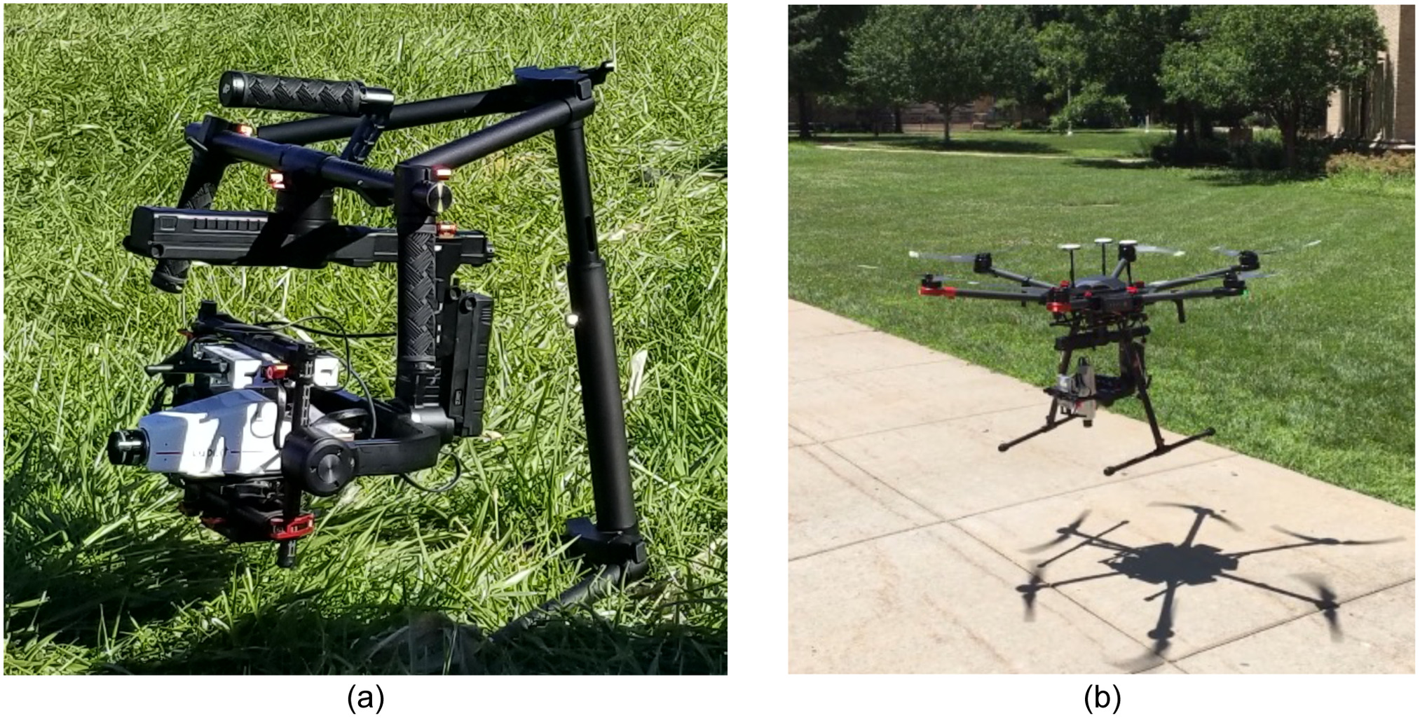
The camera has a working wavelength range of 450–950 nm, covering the visible and near-infrared (VNIR) wavelengths, spanning 139 bands, with a spectral resolution of 4 nm at each band. Although the camera natively captures radiance values, the onboard computer can output reflectance images through a proper calibration and processing process. Through a sharpening process, the camera can fuse the spectral pixels with low spatial resolution () and the accompanying grey-level image with high resolution (). A simple preprocessing step is applied that removes the first and last five spectral bands to avoid significant imaging noises at these bands. In this work, the resulting hyperspectral cubes have a dimension of (). In addition to the hyperspectral cubes, the camera produces a panchromatic (grey) image associated with each hyperspectral cube. This grey image is used as the basis for annotating a hyperspectral cube, generating a segmentation mask image. In addition, at each imaging site, a smartphone-based color image is captured as a visual reference for conducting the annotation.
The dataset adopted in this work comes from 50 original hyperspectral images, which were captured from two structural material scenes: asphalt pavements (16 images) and concrete pavement or structures (34 images). It is emphasized that this imagery dataset is much smaller than the regular datasets used in the latest image-based damage detection efforts using DL approaches. Within each hyperspectral cube, pixel-level labeling through a manual (naked-eye) segmentation was conducted over the grey image with the assistance of the smartphone color image. A total number of eight surface material types and structural conditions are considered, including structural cracks, oil spills, watermarks or moisture, dry vegetation or fungi, green vegetation or fungi, artificial marks, graffiti or other colored stains, asphalt, and concrete (Chen 2020).
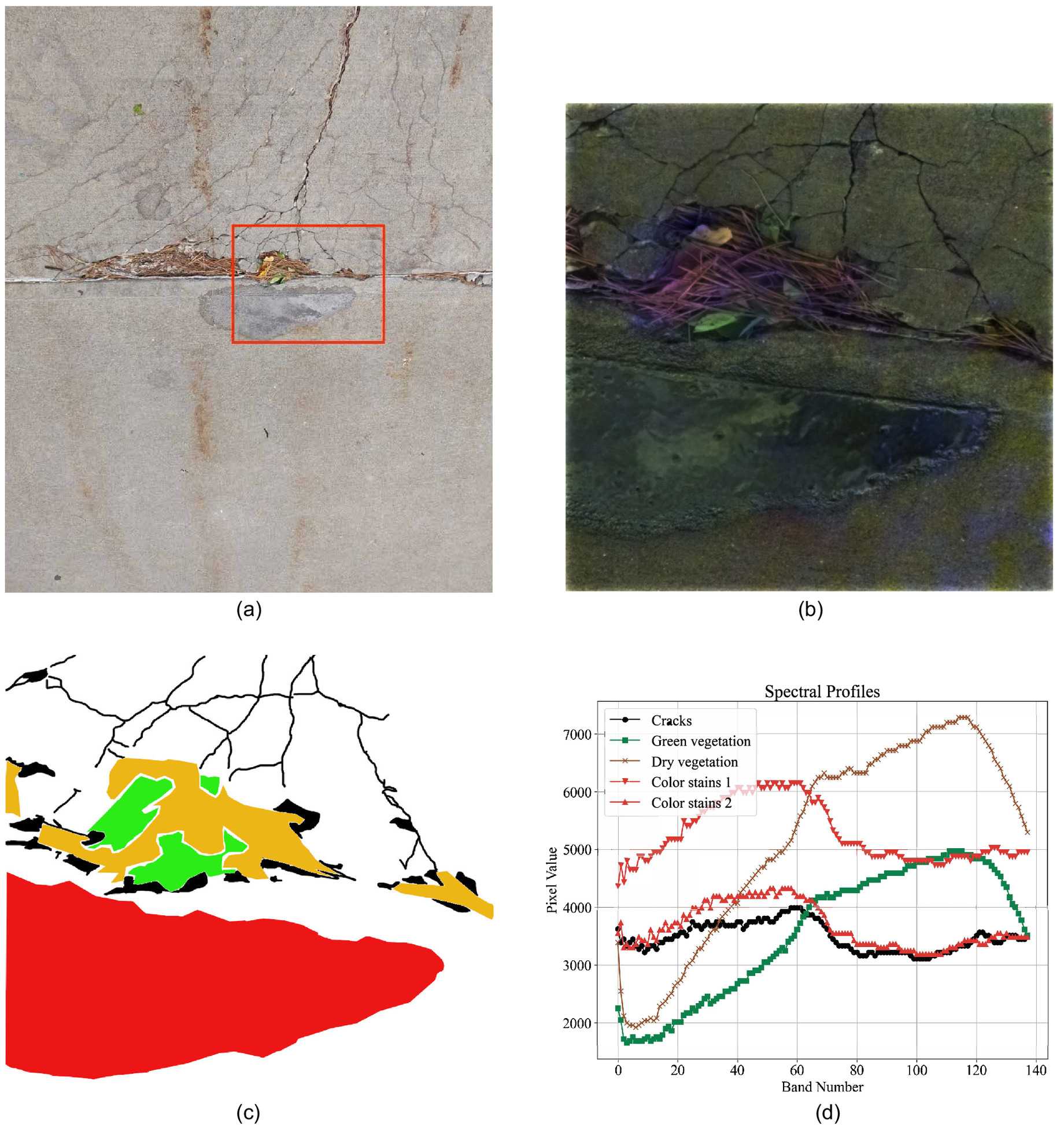
Fig. 2 illustrates one representative imaging instance. In Fig. 2(a), the scene from the use of a smartphone color image is shown. The hyperspectral cube cannot be rendered directly as a printable image; Fig. 2(b) shows the pseudo-color image reconstructed with three bands extracted from the cube; Fig. 2(c) shows the color-rendered mask image from manual annotation with five different object types; and Fig. 2(d) provides sample spectral profile plots for three object types: cracks, green vegetation, dry vegetation, and color stains (two instances). First, it can be observed that the spectral profiles are well-separable for different object types. More important to note is that spectral profiles alone cannot be fully distinct for the complex scenes; the profile of the second color stains is nearly similar to the crack’s pixel’s profile. This implies and motivates the need to extract features from the spectral profiles as well as from the spatial contexts.
Two specific treatments are conducted to build the training dataset for this work.
1.
To consider the spatial dependence, a block centered at each pixel with the spatial size of is extracted. Therefore, each data point is defined as a matrix with its center spectral pixel as its representative profile.
2.
To accommodate the proposed spatial-spectral DL and the HITL mechanism in this work, hyperspectral pixels and their labels are preselected with approximately equal quantities. By randomly sliding through each original hyperspectral image, a well-balanced data set with a total of 41,6932 data points and each class label having about 5,200 data points are developed for this work.
Methodology
Overview
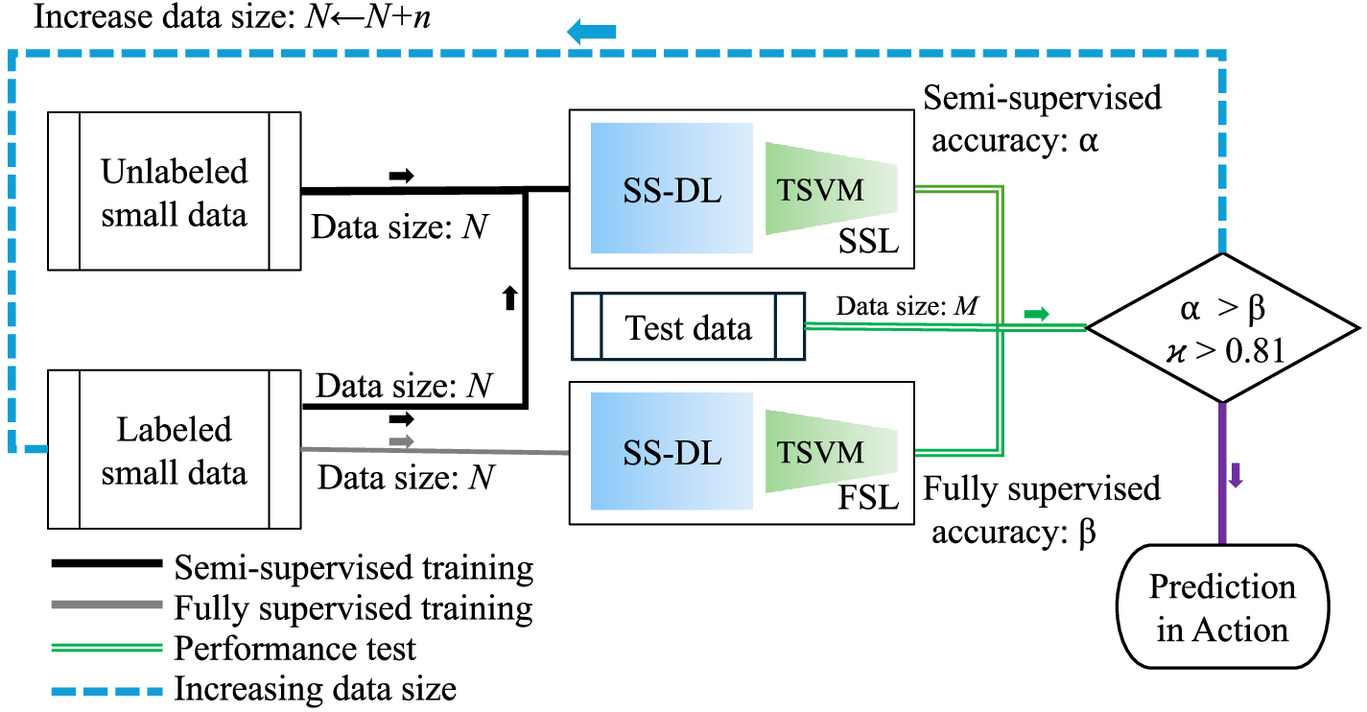
To answer the research questions, the authors propose an HITL incremental semisupervised DL framework in this work. To illustrate its distinction against a classic ML workflow, Fig. 3 provides a comparative illustration of the classic acyclic ML workflow and the proposed HITL-enabled cyclic and incremental learning workflow.
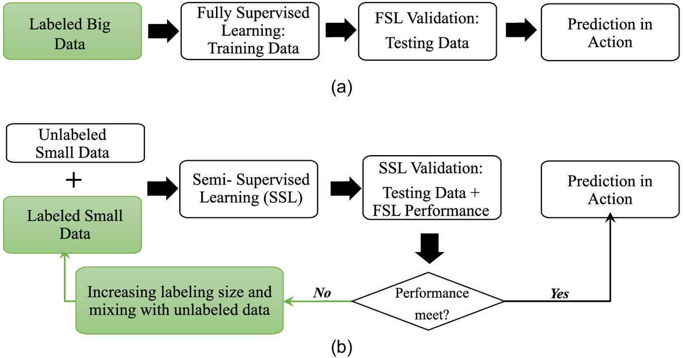
Fig. 3(a) depicts this classic ML workflow, where the human effort is “one-shot”: the human analyst prepares labeled data, and the machine (i.e., an ML classification model) learns from the data, possibly reaching the ceiling accuracy (i.e., determined by the Bayes’s error rates in the labeled data), prior to making inference or prediction in action. Fig. 3(b) illustrates the HITL methodology framework with cyclic operations. In terms of the HITL operations, besides providing initial small-sized labeled and unlabeled datasets, the major operation is to incrementally increase the training data size by repeating a semisupervised learning module until the performance is met before the prediction action.
As emphasized earlier, the untapped capacity of using hyperspectral data for structural material and damage detection is its potential accuracy that may exceed human accuracy (based on the labeling) if both labeled and unlabeled data are provided for ML model training. Two beneficial consequences can be triggered: (1) higher ML model prediction accuracy than the human analyst and (2) incrementally higher accuracy as the sizes of labeled and unlabeled data used in training increase. Besides the cyclic HITL operational workflow as shown in Fig. 3(b), a semisupervised learning architecture highly flexible for configuring the sizes of labeled and unlabeled training data is entailed.
In the following subsections, we present technical details for (1) the algorithmic semisupervised ML architecture, which includes the use of a novel SS-DL network and a semisupervised classification model using a linear TSVM, and (2) the incremental HITL strategy and resulting models with variable configurations of labeled and unlabeled training data.
Semisupervised Learning
Spatial-Spectral Feature Extraction
Necessary notations are defined based on the characteristics of hyperspectral data and pixel-level labeling described previously. First, assuming a total of data points involved in the training (including internal validation) and testing process, a hyperspectral data set is defined as . Given a , its ground-truth label is noted. Assuming that there are different class types, which are ordered as integers from 1 to , therefore, . With the spatial-spectral network extraction process described below, a vector is used to define the feature vectors extracted individually from a hyperspectral data point. Given these notations, we use as a basic labeled input and as an unlabeled input to the SS-DL network. Further, is used as a labeled feature vector input with a ground-truth label and with a pseudo-label .
The feature extraction network of the proposed SS-DL network is illustrated in Fig. 4. The architecture is designed to have two parallel feature extraction networks. The 1D CNN network aims to capture embedded features hidden in the spectral profile of a pixel. The 1D CNN has been commonly used to process time-series data in the literature (e.g., vibration or electrocardiogram data) (Kiranyaz et al. 2015; Ince et al. 2016). A neighborhood-based extraction is conducted for spatial feature extraction. In this work, a spatial size of is selected for a neighborhood. Given a data cube of , a modified ResNet50 network is adopted. ResNet50 is a variant of the originally proposed deep residual network (He et al. 2016). To date, ResNet50 is one of the most commonly used CNNs and has been adopted in many benchmarking tests (Dhillon and Verma 2020; Alzubaidi et al. 2021).
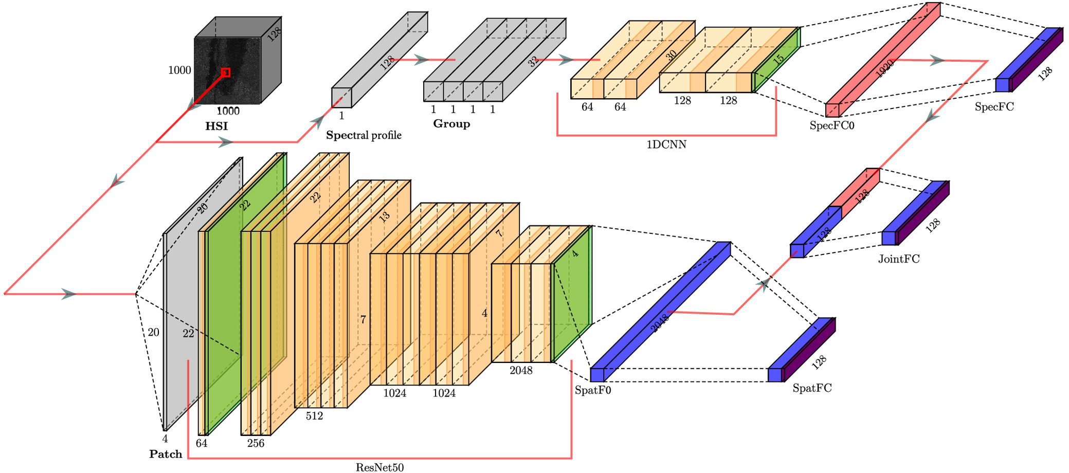
Two feature vectors are initially produced as illustrated in Fig. 4 from the parallel networks: SpatFC0 () from the spatial feature extraction network and SpecFC0 () from the spectral feature extraction network. A fully connected subnetwork is further applied to the two high-dimension vectors, leading to a spatial and a spectral feature vector component with the dimension of , termed SpatFC and SpecFC, respectively. A simple vector stacking operation is applied to the two feature components, which is further reduced to through a fully connected network, JointFC. With this treatment, three types of feature vectors, using the notations above, are obtained, denoted as , , and . The three components of spatial-spectral feature vectors are further fed into the classification layer. In a typical CNN for a multiclass classification model, it can be a dense network with a Softmax activation function. In this work, a linear TSVM is implemented to realize semisupervised learning. The design specifics are detailed as follows.
Semisupervised Classification
The technical details for the original TSVM can be found in Joachims (1999). In summary, a TSVM model attempts to determine a decision boundary that takes into account both labeled and unlabeled data points simultaneously. The optimization problem is solved for a regularized loss function that not only maximizes the decision margin (i.e., width between hyperplanes as defined in a traditional SVM), but also minimizes classification errors on both the labeled and unlabeled data. Subsequently, two specific designs are proposed in this work. The first is the creation of an appropriate loss function, and the second is the implementation of a pseudo-label updating scheme.
In general, the learning of a multiclass SVM is achieved by solving a quadratic programming problem (Crammer and Singer 2001). Given a data pair , we define a class-label dependent flag variable, with , if as a ground-truth (or pseudo-) label takes the class label, namely, ; otherwise . In a classic linear SVM, the training process is to estimate the weight vector at each class label through minimizing a regularized loss function. First, a classic hinge-loss function is defined as follows:
(1)
The multiclass linear SVM optimization is then expressed aswhere the double-summed hinge losses over data points and class labels define the total loss, scaled by a penalty parameter as a model hyperparameter, and the last term as a squared norm defines the regularization to prevent overfitting. The minimization is conducted upon all weight vectors ’s and the hyperplane intercept parameters ’s, collectively forming a model parameter matrix with a dimension of a . It is well known that an equivalent form to Eq. (2) is to introduce the regularization strength parameter to replace the convenient fraction number ½ for the regularization. If so, the penalty parameter becomes explicit as . In this work, the proposed SS-DL model has a parallel structure for simultaneously extracting spectral and spatial features. Moreover, the loss function needs to be adjusted to accommodate both labeled and unlabeled data points for semisupervised learning.
(2)
Two novel treatments are proposed in this work. First, the basic hinge loss is calculated separately based on the three feature vectors (Fig. 4), which include , , and the joint feature vector . Second, to consider a semisupervised learning process, we define as the labeled dataset (with ground-truth labels) and as the unlabeled dataset (with pseudo-labels), where and . With this configuration and the definition of hinge loss in Eq. (1), the optimization for a linear multiclass TSVM becomeswhich has two penalty parameters, and . Obviously, besides that, works as a penalty parameter for the unlabeled data, and it can be treated as a switch. If unlabeled data points are not used, by setting , then the TSVM reverts to the classic (fully supervised) SVM. Combined with the pseudo-labeling treatment during the learning process, the two hyperparameters, and , control the generalization performance of the resulting semisupervised classification model.
(3)
Pseudo-Label Updating and Semisupervised Training
The pseudo-labeling starts with the training of the SS-DL network with the labeled samples only, expressed as , which yields the initially learned model parameters . For the th hyperspectral sample without a label, its pseudo-label is assigned the first time with the label achieving the highest confidence score, as follows:where the superscripts (0) and (1) = initial learning of the model parameters and the first assignment of the pseudo-labels, respectively.
(4)
After the initial pseudo-labeling, the originally labeled and pseudo-labeled datasets are combined as one training dataset. As such, the complete model (SS-DL + TSVM) is retrained, and the model parameters are reestimated. The pseudo-labels for the unlabeled samples are then reassigned by selecting the maximal confidence scores. This process iterates until the pseudo-labels as a whole stabilize. Eq. (5) describes this pseudo-label updating process, where the superscripts () and () indicate the iteration:
(5)
For the criterion of stability, an empirical treatment is adopted. Considering the expected prediction accuracy, if less than 4% of the labels are not updated, which is treated as the error-tolerance parameter, this inner iteration process is then stopped. When such stability is achieved, the resulting pseudo-labels are considered final, and the weight matrix, , is learned from the partially labeled training data.
The training of the end-to-end model, including the SS-DL network for feature extraction and the TSVM, is realized by means of the stochastic gradient descent (SGD) learning process (Du et al. 2019). For the practical implementation, a small number of samples with ground-truth labels are reserved for the validation during the training process, denoted as . This validation process constructs the outer iteration during the training procedure. More importantly, it provides the mechanism for empirically determining the classification hyperspectral parameters and .
Incremental Learning and Operation
To answer the research questions, three DL models, hence three different incremental HITL learning schemes, are designed, following Fig. 3(b), leading to three groups of ML models. All these models use the same spatial-spectral deep neural networks for feature extraction or as the “backbone” network (Fig. 4) and a linear TSVM as the classification layer. It is the configuration of the proportion of labeled and unlabeled data during the training that leads to three different HITL schemes. In this work, one baseline is to approximately estimate the highest possible ground-truth accuracy; therefore, among the 416,932 labeled hyperspectral data points, about 99% of the samples are randomly selected for the model training, and the other 1% (4,200 data points) are used for the model testing.
By taking the total training data volume as the reference volume marked at 100%, the three groups of ML models with the incremental schemes, denoted by , , and , are described as follows. Table 1 summarizes the list of the models for each group in this work.
•
: Fully-supervised incremental learning. Using only labeled data, the proposed ML architecture with a linear TSVM reverts to a fully supervised learning model. More specifically, given the increasing sizes are 4%, 10%, …, 100% of the total training data, a series of incremental models, , … and , are obtained, respectively. It is expected that their accuracy measurements approach the underlying visual ground-truth accuracy as the training data size increases, providing the benchmark performance for verifying the semisupervised classification models.
•
: Semisupervised incremental learning with a variable participation ratio between the labeled and the unlabeled data. The resulting models start with , indicting 4% of the total training data as labeled input and 96% as unlabeled input. Accordingly, the other models include , …, and . These models are used to show (1) that semisupervised models can achieve better accuracy than the fully supervised counterparts and (2) how the participation ratio between the labeled and the unlabeled affects classification accuracy.
•
: Semisupervised models with equal participation of the labeled and unlabeled data. The resulting models start taking 4% of the total training data as labeled input and another 4% as unlabeled input. Accordingly, the models include , , …, and . As will be shown later, this empirical selection of the participation ratio is a safe choice given that a higher ratio between the unlabeled and labeled data potentially can yield higher performance. These models serve to prove the benefits of conducting HITL incremental ML, even without explicit knowledge of an optimal participation ratio between the labeled and unlabeled data.
| Fully supervised models | Semisupervised models | ||||||
|---|---|---|---|---|---|---|---|
| Labeled (%) | Models | Labeled (%) | Unlabeled (%) | Models | Labeled (%) | Unlabeled (%) | Models |
| 4 | 4 | 96 | 4 | 4 | |||
| 10 | 10 | 90 | 10 | 10 | |||
| 20 | 20 | 80 | 20 | 20 | |||
| 30 | 30 | 70 | 30 | 30 | |||
| 40 | 40 | 60 | 40 | 40 | |||
| 50 | 50 | 50 | 50 | 50 | |||
| 60 | 60 | 40 | — | — | — | ||
| 70 | 70 | 30 | — | — | — | ||
| 80 | — | — | — | — | — | — | |
| 90 | — | — | — | — | — | — | |
| 100 | — | — | — | — | — | — | |
Experimental Validation
Model Training and Inference Cost
All models were trained and tested individually following the training data schemes as listed in Table 1. The training and testing experiments were conducted using the NSF XSEDE infrastructure at the Pittsburgh Supercomputing Center (PSC). The computing resources allocated to this work include an NVIDIA Tesla V100 GPU node with 16 GB of GPU memory, two Intel Xeon Gold 6148 CPUs with , and 192 GB RAM, all on an HPE Apollo 6500 virtual server.
As for training time, it highly depends on the selection of batch sizes, learning rates, and their adjustment during the training process. Nonetheless, thanks to the proposed incremental semisupervised learning scheme, one computing advantage is to exploit the trained models in sequence. As the models share the same deep-neural network as the feature extraction backbone, the network largely learns the discriminative features of different classes from the first (fully supervised) learning. By introducing unlabeled data incrementally due to the HITL framework, the training process is a fine-tuning step and the training time is much reduced. In our experiment, the first set of models (’s as shown in Table 1, took 2 to 6 h); the ensuing semisupervised models cost less than a fifth to a tenth of the initial training time.
From Figs. 5(b–f), a set of prediction results from different models, including , , , , and , are rendered as color maps. Visually, it is challenging to assess which model provides the most accurate prediction compared with the ground truth shown in Fig. 5(a).
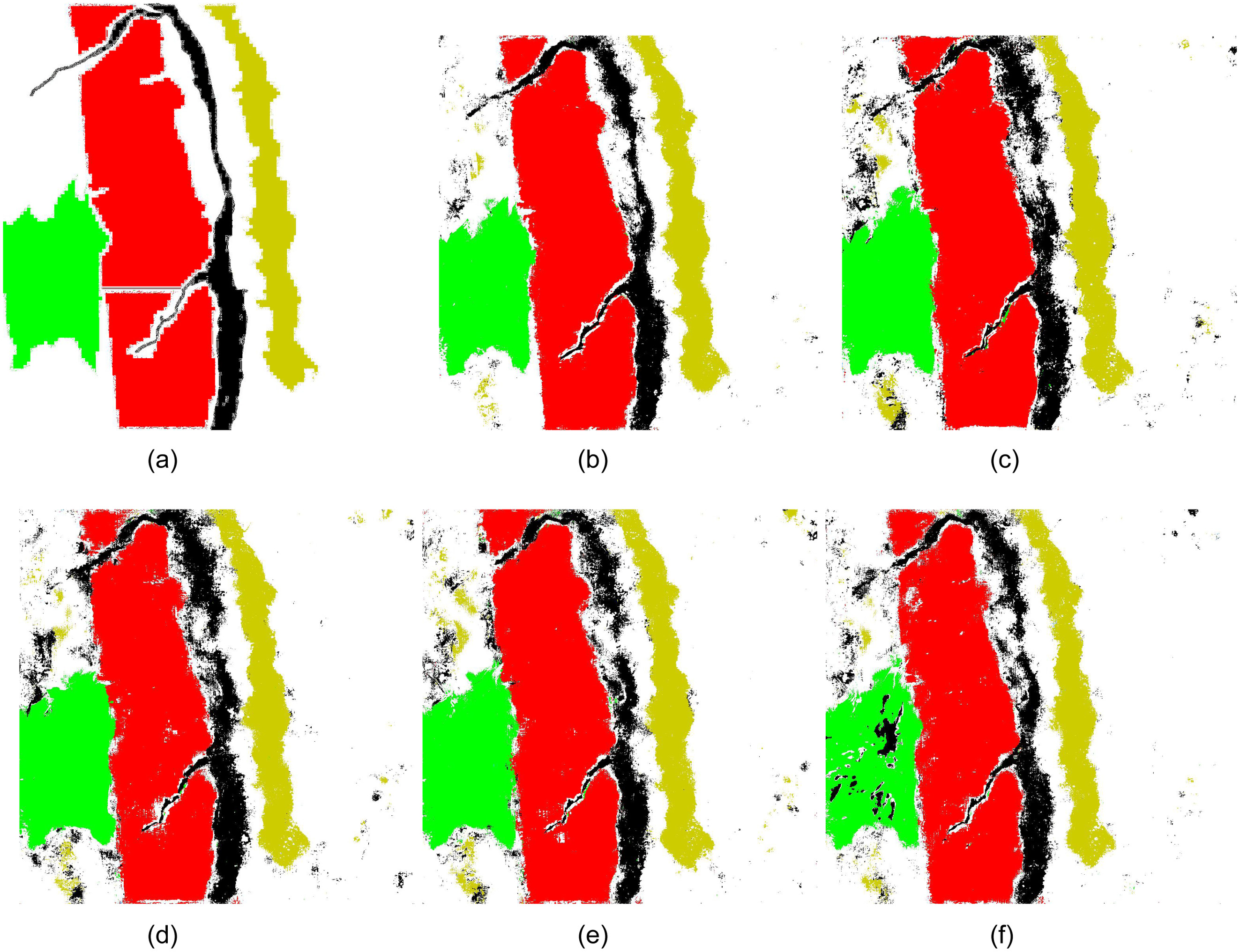
Nonetheless, one significant result arising from making a prediction given an input image, as shown in Fig. 5, is that the inference time is very close, all around 400 s for one image ( hyperspectral pixels), regardless of the underlying fully supervised or semisupervised model, due to their shared deep spatial-spectral neural network structures as the common backbone.
Performance Measures
With the testing data, the confusion matrices for individual models are computed. Given a confusion matrix, two performance measures are adopted. The primary one is the overall accuracy (OA), which defines the proportion of correctly classified samples out of all samples over all classes. Due to the underlying balance in the dataset (i.e., approximately the same number of instances at each object class), an OA measure has no skew toward a particular class. In addition, there is no consideration of weighted costs for the classification errors. Therefore, other common measures, including precision and recall for individual classes, are not adopted; we observed that the trends of the average precision and recall are consistent with the OA.
The second measure is the Cohen’s kappa statistic (). The statistic is a classic measure to evaluate the performance of a classification model compared to a human rater who provides the ground-truth labels from manual annotation. Analytically, compared with the OA measure, the measure is computed not only considering the correct predictions but also factoring in the incorrect predictions and their interplay. Therefore, the measure offers a consistency check between the different parametric classifiers from the same model architecture (McHugh 2012), which are more meaningful considering the various classification models shown in Table 1. The statistic ranges from to 1: a negative value indicates that the classifier overall disagrees with the human rater, zero means that it is no better than a random classifier, a positive value indicates partial agreement with the human rater, and indicates a perfect agreement.
Incremental Fully Supervised Learning
The achieved accuracy measurements for the fully supervised models, in terms of OA and , are listed in Table 2. Basically, and OA manifest an improving trend along the increasing size of the labeled data. On the other hand, our strategy of adopting well-balanced training data is demonstrated by the consistency between the OA and measurements.
| Measure | |||||||||||
|---|---|---|---|---|---|---|---|---|---|---|---|
| OA (%) | 67.8 | 73.4 | 74.2 | 81.5 | 86.2 | 86.3 | 87.9 | 90.2 | 90.7 | 90.6 | 92.3 |
| 0.631 | 0.696 | 0.706 | 0.788 | 0.842 | 0.843 | 0.862 | 0.888 | 0.894 | 0.893 | 0.912 |
Especially, the OA’s increasing trends can be roughly grouped into three phases based on the use of training data size: with the training data size less than 30%, with the training data size between , and when the training data size is beyond 70%. The final OA score is rated at 92.3%, which is treated as the maximal accuracy from the fully supervised models. The statistic reveals a similar conclusion; moreover, if the common rating criterion is used if or when the training data size is over 40%, the two raters—the classification model and the human rater—have achieved nearly perfect agreement (McHugh 2012).
Incremental Semisupervised Learning with Variable Participation
By utilizing the complete training dataset while one portion is used as labeled input and the other as unlabeled, a total of eight models are trained and tested. Similar to the fully supervised models, the resulting performance based on the independent testing data is reported in Table 3. Besides the OA and measurements, the difference in the accuracy measures between a model and its counterpart fully supervised model with the same amount labeled training data are reported; for example is calculated between OA from the model and . To visualize the performance measurements, Fig. 6(a) comparatively illustrates the performance trends from the two sets of models in terms of the OA and measures separately.
| Measure | ||||||||
|---|---|---|---|---|---|---|---|---|
| 24 | 9 | 4 | 2.3 | 1.5 | 1 | 0.67 | 0.43 | |
| OA (%) | 65.24 | 73.73 | 83.42 | 86.35 | 88.84 | 88.51 | 86.85 | 89.61 |
| (%) | 0.39 | 12.38 | 5.98 | 3.06 | 2.61 | |||
| 0.6027 | 0.6997 | 0.8105 | 0.8439 | 0.8725 | 0.8686 | 0.8497 | 0.8813 | |
| (%) | 0.47 | 14.89 | 5.57 | 7.05 | 3.58 |
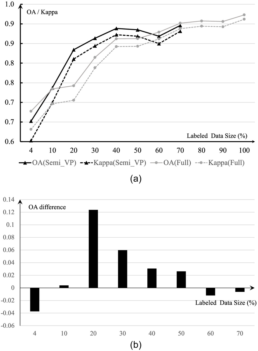
In Fig. 6(a), as the labeled data portion increases from 4% to 70% and the unlabeled data sizes decreases from 96% to 30%, the overall accuracy of the models ascend first till the model , then slightly decreases at the model , increases again. The statistic (denoted as Kappa in the figure) exhibits the same trend. By comparing the model performance within ’s, this trend reflects the role of unlabeled data in the learning task. Fig. 6(b) illustrates the performance gain or loss between the models and the models along the size of the labeling data. The trend is apparent to indicate that the presence of unlabeled data, starting with a negative contribution (performance loss) with 96% of data being unlabeled, shows its positive contribution at 90%, peaking the contribution at 80%. Then, its contribution decreases as the unlabeled data size increases. The performance loss is observed again when the labeled data dominates or the unlabeled data are less than 40%.
These observations reveal that the semisupervised models ’s can achieve better accuracy than the fully supervised counterparts with the same amount of labeled data. The unanswered question is if there is an optimal ratio between the labeled and the unlabeled data portions, such that the semisupervised models achieve the best performance. From Table 3, given the ratio values ’s between the unlabeled and the labeled data, two main facts are observed: (1) the performance of models is peaked at the cases of for the labeled and unlabeled data ratios, and (2) the performance gain compared against models stops at the ratio of .
This ratio of or is adopted as a conservative participating ratio used for the following test of the semisupervised models with equal participation, namely, ’s.
Semisupervised Learning with Equal Participation
Following the format of presenting the performance of ’s, Table 4 reports the accuracy measurements and accuracy gains compared with the fully supervised models. Fig. 7 visualizes the results in Table 4.
| Measure | ||||||
|---|---|---|---|---|---|---|
| OA(%) | 69.51 | 73.87 | 77.04 | 85.56 | 87.24 | 88.51 |
| (%) | 2.585 | 0.59 | 3.79 | 5.00 | 1.19 | 2.61 |
| 0.6515 | 0.7014 | 0.7376 | 0.8349 | 0.8541 | 0.8686 | |
| (%) | 3.17 | 0.70 | 4.55 | 5.91 | 1.39 | 3.06 |
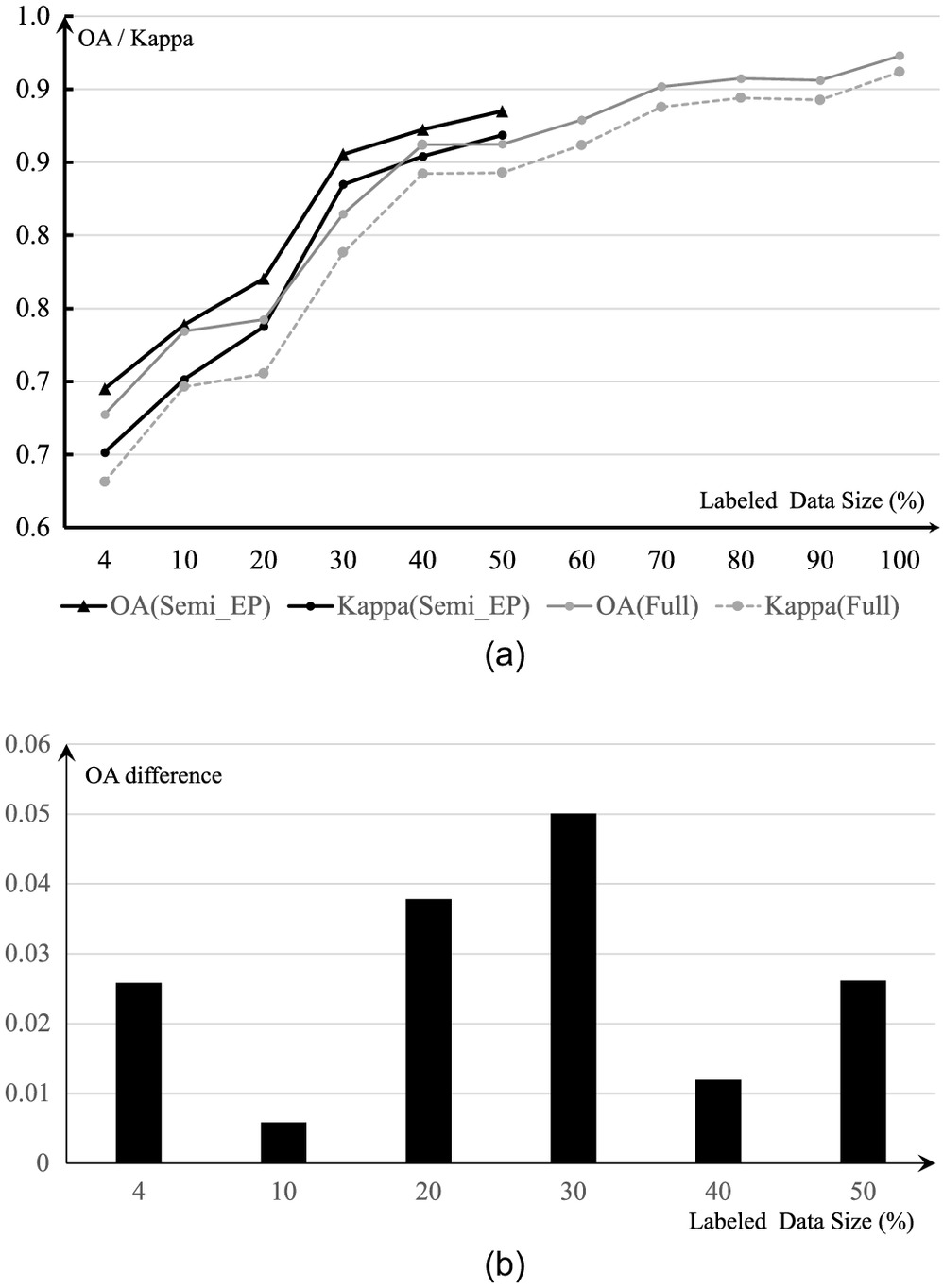
As shown in Fig. 7(a), the semisupervised models with equal participation between the labeled data and the unlabeled data overall achieved better accuracy than the fully supervised counterpart models. After reaching the total training data size of 60% at , the statistic reaches 83.49%, showing a very acceptable performance compared with the human rater. Fig. 7(b) provides the performance gain as the training data size increases. It is apparent that there is no overall trend of performance gain when the ratio between the unlabeled and labeled data in training is kept equal. The model of approaches the maximal improvement; the others on the two sides have less accuracy improvement.
Two important messages are revealed and summarized based on the ML scheme of using the ’s model series.
•
The assessment above reveals that the semisupervised learning model can improve the classification performance compared to the supervised learning model when using a training data set of the same size.
•
This configuration of ratio between the unlabeled and labeled data in training proves to be a conservative yet consistent semisupervised learning strategy.
Discussion
The comparative numerical studies on the performance of three incremental learning strategies reveal the feasibility of conducting HSI-based structural materials and damage detection in parallel with an HITL operation workflow. By comparing the performance trajectories of the fully supervised models ’s and the semisupervised models with equal participation ’s, an empirical operation workflow is recommended, as summarized in Fig. 8, and the major operations are discussed below.
First, a human analyst may start with minimal labeling to initiate the process. As implied in Fig. 8, the analyst may select a few hyperspectral cubes and use the panchromatic image as the mask candidate to start the pixel labeling. For this purpose, modern annotation tools are abundant and free to use. In this work, the initial labeled data size is about 4% of the maximal training data size, or about 15,000 pixels, which essentially is about 1.5% of a hyperspectral cube image (which boasts or one million pixels), and a few thousand of labeled pixels as testing data (in this work, 4,000 labeled pixels are used in testing). By taking another 15,000 unlabeled pixels to mix with the labeled one, the initial semisupervised training can begin. Thanks to the flexibility of the TSVM model, without using the unlabeled data points, it is reduced to a fully supervised model that produces inference results for benchmarking.
Second, the analyst makes high-level decisions in the HITL loop until the production action is taken.
•
When the training-testing operation starts, the testing data based performance (denoted as ) should be compared against the performance () of the fully supervised model.
•
If the results are that the semisupervised model exceeds the fully supervised model (), it is an expected result that the semisupervised model exploits hidden structure in the unlabeled data. If not, careful diagnosis should be conducted.
•
With the expected semisupervised model performance, it proceeds with determining if the accuracy meets the expectation. Besides the comparison of , the statistic can be used as a straightforward criterion; when , it can be accepted, and the model is ready for production or prediction in action. If not, the analyst should continue to provide labeled data and an equal amount of unlabeled data for the incremental semisupervised training. Then, the loop ends until the production action is taken.
One limitation of this work is to determine an analytical range for the possible ratios of unlabeled data and labeled data toward an optimal semisupervised learning performance. Our studies are empirical and ad-hoc using the hyperspectral data prepared for this work. From Table 1, it seems that the range is high (i.e., the is within ), and the trend is not monotonic. The selection of the ratio of in this work is a conservative decision away from a possibly optimal decision. In the literature, most researchers assume a larger amount of unlabeled data along with a small amount of labeled data, i.e., , to train and test semisupervised ML models (Van Engelen and Hoos 2020; Yang et al. 2023). However, no study or method exists that confirms or leads to a fixed ratio, as it is generally believed that the ratio can vary widely depending on several factors, including the specific task, the nature of the data, and the chosen algorithm. We leave the possibility of using a larger ratio of unlabeled data and labeled data in future work using the proposed parametric SS-DL and TSVM architecture.
Last, this work aims to develop an operational framework, i.e., HITL-based semisupervised deep learning, and it has been tested with a complex dataset that comes from two different structural materials with significant scene complexities. Regardless, the achieved models in this work are ad-hoc for the dataset in this work only. To scale or to generalize to a different setting, including the use of a larger dataset or consideration of a different civil structures or infrastructure scene, the proposed methodology, shown in Fig. 8, can be readily adopted.
Practical Applications
In this work, an HSI-enabled machine-vision workflow is developed for civil infrastructure inspection. Compared with regular (e.g., color images with red, green, and blue bands), the use of HSI can effectively deal with the scene complexity issues that are often encountered in practice (e.g., pavement or structural surfaces that show environmental artifacts besides showing signs of damage). Besides its hallmark of using hyperspectral images, the workflow integrates two novel design features: semisupervised ML and HITL operation. Semisupervised learning, while enabling the use of small data to initiate the learning process, can unfold the potential power of hyperspectral images and provide detection accuracy beyond human vision. The HITL operation places end users in the decision-making process, rendering the use of unlabeled data. For a specific type of inspection scene, the proposed methodology can be adopted to develop a software-based workflow in conjunction with a modern hyperspectral camera, which can be further installed in an aerial or ground robotic vehicle, hence realizing inspection automation.
Conclusions
The main contributions of this work are two-fold: the exploration of semisupervised deep learning, a semisupervised learning scheme, and an operational workflow where incremental machine learning is proposed and tested. Such a contribution may positively impact the field of machine vision-enabled structural and infrastructure condition inspection. To this end, the majority of the efforts use regular or color images, with labor-intensive large-scale labeling and a larger-scale DL-based detection model. The proposed HITL incremental learning with hyperspectral images is expected to significantly improve the detection accuracy in complex scenes that can only be separable in terms of high-dimensional spectral pixels with spatial contexts. With the use of a small volume of labeled data and unlabeled datasets, the HITL workflow can be empirically determined by a human analyst to end at an acceptable level before the possible waste of labeling efforts.
Technically, with the comparative studies of three numerical experiments, we conclude with three primary findings:
1.
Fully supervised learning determines the baseline of the detection performance. In this work, fully supervised models, ’s, provide consistent accuracy improvement as the analyst increases the size of the training data. We assert that this accuracy approaches the underlying ground-truth accuracy provided by the human rater (who annotates the hyperspectral images based on the assistance of panchromatic and natural scene images); however, it does not reveal the true possible accuracy limit (the “ceiling” accuracy) within the labeled hyperspectral data.
2.
There exists a large range of ratio values between the unlabeled and the labeled data for incremental semisupervised learning. Within the range of as shown in Table 3, the semisupervised learning achieves higher accuracy values than the fully supervised models. In addition, we observed that with a too-small ratio (e.g., 0.67 or lower) or a too-high ratio (e.g., greater than 9), degraded performance can be achieved. A ratio is taken as a conservative and operational ratio.
3.
With parametric semisupervised learning with equal labeled and unlabeled data participation, the proposed HITL operational workflow can be implemented to be an effective approach for hyperspectral images based on structural material and damage detection. Although, in practice, a higher ratio can be used between the unlabeled data and the labeled data, this perspective is left to a user’s decision and is subject to future exploration.
Data Availability Statement
All data and models generated or used during the study appear in the published article. The hyperspectral imaging dataset used in this study is publicly shared through Figshare (Chen 2020).
Acknowledgments
This material is based partially upon work supported by the National Science Foundation (NSF) under Award number No. IIA-1355406 and work supported by the United States Department of Agriculture’s National Institute of Food and Agriculture (USDA-NIFA) under Award No. 2015-68007-23214. Shimin Tang contributed equally to this work. Any opinions, findings, conclusions, or recommendations expressed in this material are those of the authors and do not necessarily reflect the views of NSF or USDA-NIFA.
References
Agnisarman, S., S. Lopes, K. C. Madathil, K. Piratla, and A. Gramopadhye. 2019. “A survey of automation-enabled human-in-the-loop systems for infrastructure visual inspection.” Autom. Constr. 97 (Dec): 52–76. https://doi.org/10.1016/j.autcon.2018.10.019.
Alzubaidi, L., J. Zhang, A. J. Humaidi, A. Al-Dujaili, Y. Duan, O. Al-Shamma, J. Santamara, M. A. Fadhel, M. Al-Amidie, and L. Farhan. 2021. “Review of deep learning: Concepts, CNN architectures, challenges, applications, future directions.” J. Big Data 8 (Dec): 1–74. https://doi.org/10.1186/s40537-021-00444-8.
Aryal, S., Z. Chen, and S. Tang. 2021. “Mobile hyperspectral imaging for material surface damage detection.” J. Comput. Civ. Eng. 35 (1): 04020057. https://doi.org/10.1061/(ASCE)CP.1943-5487.0000934.
Belkin, M., and P. Niyogi. 2004. “Semisupervised learning on Riemannian manifolds.” Mach. Learn. 56 (1): 209–239. https://doi.org/10.1023/B:MACH.0000033120.25363.1e.
Bennett, K., and A. Demiriz. 1999. “Semisupervised support vector machines.” In Advances in neural information processing systems, 368–374. La Jolla, CA: Neural Information Processing Systems Foundation.
Bishop, C. 2006. Pattern recognition and machine learning. New York: Springer.
Browne, M., and S. S. Ghidary. 2003. “Convolutional neural networks for image processing: An application in robot vision.” In Proc., Australasian Joint Conf. on Artificial Intelligence, 641–652. New York: Springer.
Chen, Y., H. Jiang, C. Li, X. Jia, and P. Ghamisi. 2016. “Deep feature extraction and classification of hyperspectral images based on convolutional neural networks.” IEEE Trans. Geosci. Remote Sens. 54 (10): 6232–6251. https://doi.org/10.1109/TGRS.2016.2584107.
Chen, Y., K. Zhu, L. Zhu, X. He, P. Ghamisi, and J. A. Benediktsson. 2019. “Automatic design of convolutional neural network for hyperspectral image classification.” IEEE Trans. Geosci. Remote Sens. 57 (9): 7048–7066. https://doi.org/10.1109/TGRS.2019.2910603.
Chen, Z. 2020. “Hyperspectral imagery for material surface damage.” Figshare. Accessed May 29, 2020. https://doi.org/10.6084/m9.figshare.12385994.v1.
Chen, Z., R. Derakhshani, C. Halmen, and J. T. Kevern. 2011. “A texture-based method for classifying cracked concrete surfaces from digital images using neural networks.” In Proc., 2011 Int. Joint Conf. on Neural Networks, 2632–2637. New York: IEEE. https://doi.org/10.1109/IJCNN.2011.6033562.
Chien, C., W. Martin, A. Meyer, and J. Aggarwal. 1983. Detection of cracks on highway pavements. Austin, TX: Univ. of Texas at Austin.
Crammer, K., and Y. Singer. 2001. “On the algorithmic implementation of multiclass kernel-based vector machines.” J. Mach. Learn. Res. 2 (12): 265–292. https://doi.org/10.5555/944790.944813.
Cubert. 2022. “Hyperspectral vnir camera firefleye 185.” Cubert GmbH. Accessed January 1, 2022. https://www.cubert-hyperspectral.com/products/firefleye-185.
Cui, R., H. Yu, T. Xu, X. Xing, X. Cao, K. Yan, and J. Chen. 2022. “Deep learning in medical hyperspectral images: A review.” Sensors 22 (24): 9790. https://doi.org/10.3390/s22249790.
Dhillon, A., and G. K. Verma. 2020. “Convolutional neural network: A review of models, methodologies and applications to object detection.” Prog. Artif. Intell. 9 (2): 85–112. https://doi.org/10.1007/s13748-019-00203-0.
Didaci, L., G. Fumera, and F. Roli. 2012. “Analysis of co-training algorithm with very small training sets.” In Proc., Joint IAPR Int. Workshops on Statistical Techniques in Pattern Recognition (SPR) and Structural and Syntactic Pattern Recognition (SSPR), 719–726. New York: Springer.
Ding, S., Z. Zhu, and X. Zhang. 2017. “An overview on semisupervised support vector machine.” Neural Comput. Appl. 28 (5): 969–978. https://doi.org/10.1007/s00521-015-2113-7.
Du, S., J. Lee, H. Li, L. Wang, and X. Zhai. 2019. “Gradient descent finds global minima of deep neural networks.” In Proc., 36th Int. Conf. on Machine, 1675–1685. Breckenridge, CO: Proceedings of Machine Learning Research.
Ehrenberg, H. R., J. Shin, A. J. Ratner, J. A. Fries, and C. Ré. 2016. “Data programming with ddlite: Putting humans in a different part of the loop.” In Proc., Workshop on Human-In-the-Loop Data Analytics, 1–6. New York: Association for Computing Machinery. https://doi.org/10.1145/2939502.2939515.
Feng, F., W. Li, Q. Du, and B. Zhang. 2017. “Dimensionality reduction of hyperspectral image with graph-based discriminant analysis considering spectral similarity.” Remote Sens. 9 (4): 323. https://doi.org/10.3390/rs9040323.
Fiebrink, R., P. R. Cook, and D. Trueman. 2011. “Human model evaluation in interactive supervised learning.” In Proc., SIGCHI Conf. on Human Factors in Computing Systems, 147–156. New York: Association for Computing Machinery. https://doi.org/10.1145/1978942.1978965.
Fralick, S. 1967. “Learning to recognize patterns without a teacher.” IEEE Trans. Inf. Theory 13 (1): 57–64. https://doi.org/10.1109/TIT.1967.1053952.
Gao, L., J. Li, M. Khodadadzadeh, A. Plaza, B. Zhang, Z. He, and H. Yan. 2014. “Subspace-based support vector machines for hyperspectral image classification.” IEEE Geosci. Remote Sens. Lett. 12 (2): 349–353. https://doi.org/10.1109/LGRS.2014.2341044.
Haas, C., H. Shen, W. Phang, and R. Haas. 1984. “Application of image analysis technology to automation of pavement condition surveys.” In Proc., Int. Transport Congress, 55–73. Cape Town, South Africa: A. A. Balkema.
Haut, J. M., M. E. Paoletti, J. Plaza, J. Li, and A. Plaza. 2018. “Active learning with convolutional neural networks for hyperspectral image classification using a new Bayesian approach.” IEEE Trans. Geosci. Remote Sens. 56 (11): 6440–6461. https://doi.org/10.1109/TGRS.2018.2838665.
He, K., X. Zhang, S. Ren, and J. Sun. 2016. “Deep residual learning for image recognition.” In Proc., IEEE Conf. on Computer Vision and Pattern Recognition, 770–778. New York: IEEE.
Ince, T., S. Kiranyaz, L. Eren, M. Askar, and M. Gabbouj. 2016. “Real-time motor fault detection by 1-d convolutional neural networks.” IEEE Trans. Ind. Electron. 63 (11): 7067–7075. https://doi.org/10.1109/TIE.2016.2582729.
Joachims, T. 1999. “Transductive inference for text classification using support vector machines.” In Vol. 99 of Proc., 16th Int. Conf. on Machine Learning, 200–209. San Francisco: Morgan Kaufmann Publishers. https://doi.org/10.5555/645528.657646.
Khodadadzadeh, M., J. Li, A. Plaza, and J. M. Bioucas-Dias. 2014. “A subspace-based multinomial logistic regression for hyperspectral image classification.” IEEE Geosci. Remote Sens. Lett. 11 (12): 2105–2109. https://doi.org/10.1109/LGRS.2014.2320258.
Kim, B. 2015. “Interactive and interpretable machine learning models for human machine collaboration.” Ph.D. thesis, Dept. of Aeronautics and Astronautics, Massachusetts Institute of Technology.
Kingma, D. P., S. Mohamed, D. Jimenez Rezende, and M. Welling. 2014. “Semisupervised learning with deep generative models.” In Advances in neural information processing systems, 27. La Jolla, CA: Neural Information Processing Systems Foundation.
Kiranyaz, S., T. Ince, and M. Gabbouj. 2015. “Real-time patient-specific ecg classification by 1-d convolutional neural networks.” IEEE Trans. Biomed. Eng. 63 (3): 664–675. https://doi.org/10.1109/TBME.2015.2468589.
Kirillov, A., et al. 2023. “Segment anything.” In Proc., IEEE/CVF Int. Conf. on Computer Vision, 4015–4026. New York: IEEE.
Krishnan, S., M. J. Franklin, K. Goldberg, J. Wang, and E. Wu. 2016. “Activeclean: An interactive data cleaning framework for modern machine learning.” In Proc., 2016 Int. Conf. on Management of Data, 2117–2120. New York: IEEE.
LeCun, Y., P. Haffner, L. Bottou, and Y. Bengio. 1999. “Object recognition with gradient-based learning.” In Shape, contour and grouping in computer vision, 319–345. New York: Springer.
Lee, H., and H. Kwon. 2017. “Going deeper with contextual CNN for hyperspectral image classification.” IEEE Trans. Image Process. 26 (10): 4843–4855. https://doi.org/10.1109/TIP.2017.2725580.
Lee, J. S., Y. Ham, H. Park, and J. Kim. 2022. “Challenges, tasks, and opportunities in teleoperation of excavator toward human-in-the-loop construction automation.” Autom. Constr. 135 (Jun): 104119. https://doi.org/10.1016/j.autcon.2021.104119.
Li, S., W. Song, L. Fang, Y. Chen, P. Ghamisi, and J. A. Benediktsson. 2019. “Deep learning for hyperspectral image classification: An overview.” IEEE Trans. Geosci. Remote Sens. 57 (9): 6690–6709. https://doi.org/10.1109/TGRS.2019.2907932.
Liu, Y., Y. Zhang, Y. Wang, F. Hou, J. Yuan, J. Tian, Y. Zhang, Z. Shi, J. Fan, and Z. He. 2024. “A survey of visual transformers.” IEEE Trans. Neural Networks Learn. Syst. 35 (6): 7478–7498. https://doi.org/10.1109/TNNLS.2022.3227717.
Liu, Z., S. A. Suandi, T. Ohashi, and T. Ejima. 2002. “Tunnel crack detection and classification system based on image processing.” In Vol. 4664 of Machine vision applications in industrial inspection X, 145–153. Bellingham, WA: International Society for Optics and Photonics.
Mäkinen, S., H. Skogström, E. Laaksonen, and T. Mikkonen. 2021. “Who needs MLOps: What data scientists seek to accomplish and how can MLOps help.” In Proc., 2021 IEEE/ACM 1st Workshop on AI Engineering-Software Engineering for AI (WAIN), 109–112. New York: IEEE.
McHugh, M. L. 2012. “Interrater reliability: The kappa statistic.” Biochem. Med. 22 (3): 276–282. https://doi.org/10.11613/BM.2012.031.
Mohan, A., and S. Poobal. 2017. “Crack detection using image processing: A critical review and analysis.” Alexandria Eng. J. 57 (2): 787–798. https://doi.org/10.1016/j.aej.2017.01.020.
Mosqueira-Rey, E., E. Hernández-Pereira, D. Alonso-Ros, J. Bobes-Bascarán, and Á. Fernández-Leal. 2023. “Human-in-the-loop machine learning: A state of the art.” Artif. Intell. Rev. 56 (4): 3005–3054. https://doi.org/10.1007/s10462-022-10246-w.
Niazmardi, S., S. Homayouni, and A. Safari. 2013. “An improved fcm algorithm based on the svdd for unsupervised hyperspectral data classification.” IEEE J. Sel. Top. Appl. Earth Obs. Remote Sens. 6 (2): 831–839. https://doi.org/10.1109/JSTARS.2013.2244851.
Oullette, R., M. Browne, and K. Hirasawa. 2004. “Genetic algorithm optimization of a convolutional neural network for autonomous crack detection.” In Vol. 1 of Proc., 2004 Congress on Evolutionary Computation (IEEE Cat. No. 04TH8753), 516–521. New York: IEEE.
Pavia, D. L., G. M. Lampman, G. S. Kriz, and J. A. Vyvyan. 2014. Introduction to spectroscopy. 5th ed. Boston, MA: Cengage Learning.
Peng, B., C. Li, P. He, M. Galley, and J. Gao. 2023. “Instruction tuning with gpt-4.” Preprint, submitted April 6, 2023. https://arxiv.org/abs/2304.03277.
Rasti, B., D. Hong, R. Hang, P. Ghamisi, X. Kang, J. Chanussot, and J. A. Benediktsson. 2020. “Feature extraction for hyperspectral imagery: The evolution from shallow to deep: Overview and toolbox.” IEEE Geosci. Remote Sens. 8 (4): 60–88. https://doi.org/10.1109/MGRS.2020.2979764.
Ritchie, S. G. 1990. “Digital imaging concepts and applications in pavement management.” J. Transp. Eng. 116 (3): 287–298. https://doi.org/10.1061/(ASCE)0733-947X(1990)116:3(287).
Scudder, H. 1965. “Probability of error of some adaptive pattern-recognition machines.” IEEE Trans. Inf. Theory 11 (3): 363–371. https://doi.org/10.1109/TIT.1965.1053799.
Signoroni, A., M. Savardi, A. Baronio, and S. Benini. 2019. “Deep learning meets hyperspectral image analysis: A multidisciplinary review.” J. Imaging 5 (5): 52. https://doi.org/10.3390/jimaging5050052.
Tang, Y. Y., H. Yuan, and L. Li. 2014. “Manifold-based sparse representation for hyperspectral image classification.” IEEE Trans. Geosci. Remote Sens. 52 (12): 7606–7618. https://doi.org/10.1109/TGRS.2014.2315209.
Theodoridis, S., and K. Koutroumbas. 1999. “Pattern recognition and neural networks.” In Advanced course on artificial intelligence, 169–195. New York: Springer.
Van Engelen, J. E., and H. H. Hoos. 2020. “A survey on semisupervised learning.” Mach. Learn. 109 (2): 373–440. https://doi.org/10.1007/s10994-019-05855-6.
Vapnik, V. 1999. The nature of statistical learning theory. New York: Springer.
Windrim, L., A. Melkumyan, R. J. Murphy, A. Chlingaryan, and R. Ramakrishnan. 2018. “Pretraining for hyperspectral convolutional neural network classification.” IEEE Trans. Geosci. Remote Sens. 56 (5): 2798–2810. https://doi.org/10.1109/TGRS.2017.2783886.
Wu, X., L. Xiao, Y. Sun, J. Zhang, T. Ma, and L. He. 2022. “A survey of human-in-the-loop for machine learning.” Future Gener. Comput. Syst. 135 (Mar): 364–381. https://doi.org/10.1016/j.future.2022.05.014.
Yang, X., Z. Song, I. King, and Z. Xu. 2023. “A survey on deep semisupervised learning.” IEEE Trans. Knowl. Data Eng. 35 (9): 8934–8954. https://doi.org/10.1109/TKDE.2022.3220219.
Yao, D., Z. Zhi-li, Z. Xiao-feng, C. Wei, H. Fang, C. Yao-ming, and W.-W. Cai. 2023. “Deep hybrid: Multi-graph neural network collaboration for hyperspectral image classification.” Def. Technol. 23 (Apr): 164–176. https://doi.org/10.1016/j.dt.2022.02.007.
Yu, S., S. Jia, and C. Xu. 2017. “Convolutional neural networks for hyperspectral image classification.” Neurocomputing 219 (Jun): 88–98. https://doi.org/10.1016/j.neucom.2016.09.010.
Zanzotto, F. M. 2019. “Human-in-the-loop artificial intelligence.” J. Artif. Intell. Res. 64 (Apr): 243–252. https://doi.org/10.1613/jair.1.11345.
Zhang, C., J. Shin, C. Ré, M. Cafarella, and F. Niu. 2016. “Extracting databases from dark data with deepdive.” In Proc., 2016 Int. Conf. on Management of Data, 847–859. New York: Association for Computing Machinery. https://doi.org/10.1145/2882903.2904442.
Zhang, C. J., L. Chen, H. V. Jagadish, and C. C. Cao. 2013. “Reducing uncertainty of schema matching via crowdsourcing.” Proc. VLDB Endow. 6 (9): 757–768. https://doi.org/10.14778/2536360.2536374.
Zhang, S., J. Zhang, X. Wang, J. Wang, and Z. Wu. 2023. “ELS2T: Efficient lightweight spectral-spatial transformer for hyperspectral image classification.” IEEE Trans. Geosci. Remote Sens. 61: 1–16. https://doi.org/10.1109/TGRS.2023.3299442.
Zhao, C., B. Qin, S. Feng, W. Zhu, W. Sun, W. Li, and X. Jia. 2023. “Hyperspectral image classification with multi-attention transformer and adaptive superpixel segmentation-based active learning.” IEEE Trans. Image Process 32 (Jun): 3606–3621. https://doi.org/10.1109/TIP.2023.3287738.
Zhong, Y., A. Ma, and L. Zhang. 2014. “An adaptive memetic fuzzy clustering algorithm with spatial information for remote sensing imagery.” IEEE J. Sel. Top. Appl. Earth Obs. Remote Sens. 7 (4): 1235–1248. https://doi.org/10.1109/JSTARS.2014.2303634.
Zhu, X. 2005. Semisupervised learning literature survey. Madison, WI: Univ. of Wisconsin–Madison.
Zhu, X., and Z. Ghahramani. 2002. Learning from labeled and unlabeled data with label propagation. Pittsburgh: Carnegie Mellon Univ.
Zhu, X., and A. B. Goldberg. 2009. Introduction to semi-supervised learning. Berlin: Springer.
Information & Authors
Information
Published In

Journal of Computing in Civil Engineering
Volume 38 • Issue 6 • November 2024
Copyright
This work is made available under the terms of the Creative Commons Attribution 4.0 International license, https://creativecommons.org/licenses/by/4.0/.
History
Received: Jan 8, 2024
Accepted: May 31, 2024
Published online: Aug 24, 2024
Published in print: Nov 1, 2024
Discussion open until: Jan 24, 2025
Authors
Metrics & Citations
Metrics
Citations
Download citation
If you have the appropriate software installed, you can download article citation data to the citation manager of your choice. Simply select your manager software from the list below and click Download.